Analysis of Intrusion Detection Log Data on a Scalable Environment

(1)

F

ACULDADE DE

E

NGENHARIA DA

U

NIVERSIDADE DO

P

ORTO

Analysis of Intrusion Detection Log

Data on a Scalable Environment

Rui Miguel Almeida Oliveira

Mestrado Integrado em Engenharia Informática e Computação Supervisor: Ricardo Santos Morla

(2)

c

(3)

Abstract

Computer defense systems, such as Firewalls and Intrusion Detection Systems, can block harmful traffic from reaching a network under their protection through the establishment of rules. However, not all malicious connections can be identified by rule matching. Especially those which are novel or use yet to be black-listed items such as IP addresses or TLS certificates.

In recent years, with the rise of computational power and efficiency, machine learning algo-rithms have made their way into all kinds of fields, including intrusion detection.

Traffic analysis of intrusion detection logs is thus relevant in order to understand what can be considered harmful and what can be considered normal. And, of course, the larger the traffic, the greater the amount of logs will be, which turns this situation into a big data issue.

Research has been undertaken into the detection of Distributed Denial of Service Attacks, either through log analysis, rule inference or traffic inspection. However, from the review of avail-able literature, it seems there are limited efforts to bring together the usage of machine learning techniques in a big data setup for traffic log classification.

This work presents an application able to capture large quantities of traffic log and to cross-reference it with a dataset to generate a ground-truth. From this new dataset, machine learning algorithms can be implemented and trained to distinguish regular traffic from intrusions. In this case, we focus on Distributed Denial of Service attacks.

(4)

(5)

Acknowledgments

I would like to express my gratitude to Dr. Ricardo Morla for accepting me as his pupil for this project, for his guidance throughout my final university year, and for his patience and availability when I required assistance.

All my friends who kept me sane with encouragement in my lowest moments, and shared rejoice in my finest hours.

And I’d like to thank my family for the incredible support through these years.

Rui Miguel Oliveira

(6)

(7)

List of Figures

1.1 Diagram of the solution concept. . . 2

2.1 OSI Model. . . 6

4.1 Full Application Diagram. . . 21

4.2 Conceptualization of a simple realistic protected network. . . 22

4.3 Conceptualization of a network. . . 23

(10)

(11)

List of Tables

3.1 List of each. . . 19

4.1 Virtual machine settings for each image. . . 22

4.2 Features selected from the log files. . . 26

4.3 Logistic Regression default settings on Pyspark. . . 28

4.4 Decision Tree default settings on Pyspark. . . 29

4.5 Random Forest default settings on Pyspark. . . 29

5.1 List of DDoS attacks performed on each day. . . 31

5.2 List the different labels and their proportions in the ground truth dataset. . . 32

5.3 The attack-benign traffic ration on the final dataset, for each attack percentage of the original dataset. . . 32

5.4 Results for the evaluation metrics of all algorithms. . . 33

5.5 Time spent on task completion. . . 34

(12)

(13)

Listings

4.1 The code snippet where the logs and ground truth dataframes are merged . . . 24

4.2 Code snippet of the data preparation process . . . 26

(14)

(15)

List of Symbols

ACC ACCuracy

ACK Acknowledge ADT Abstract Data Type

ANDF Architecture-Neutral Distribution Format API Application Programming Interface

AUC Area Under the Receiver Operating Characteristic Curve BD Breakdown Distance

CAD Computer-Aided Design

CASE Computer-Aided Software Engineering

CICDDoS2019 Canadian Institute for Cybersecurity Distributed Denial of Service evaluation dataset 2019

CORBA Common Object Request Broker Architecture COVID-19 COronaVIrus Disease 2019

CPU Central Processing Unit CSV Comma-Separated Values

DBSCAN Density-Based Spatial Clustering of Applications with Noise DDoS Distributed Denial of Service

DHCP Dynamic Host Configuration Protocol DoS Denial of Service

DT Decision Tree F1-s F1 score

FTP File Transfer Protocol FRG Filtering-Rule Generalization

GB Gigabytes

GHz GigaHertz HDD Hard Disk Drive

HDFS Hadoop Distributed File System HTTP HyperText Transfer Protocol ICMP Internet Control Message Protocol IP Internet Protocol

IPsec Internet Protocol Security IPv4 Internet Protocol version 4 IPv6 Internet Protocol version 6 IDS Intrusion Detection Systems IPS Intrusion Prevention Systems JSON JavaScript Object Notation LR Logistic Regression

MB Megabytes

(16)

xiv List of Symbols

MD Mahalanobis Distance

MLA Machine Learning Algorithms MLF Mining firewall Log using Frequency NAC Network Access Control

NAT Network Address Translation NB Naïve Bayes

OSI Open Systems Interconnect PCAP Packet CAPture

RAM Random Access Memory RF Random Forest

RFE Recursive Feature Elimination ROC Receiver Operating Characteristic SVM Support Vector Machine

SYN Synchronize

TCP Transmission Control Protocol TVA Tabulated Vector Approach UDP User Datagram Packet

UNCOL UNiversal COmpiler-oriented Language VPN Virtual Private Network

WAN Wide Area Network WP Weighted Precision WR Weighted Recall

WRFS Weighted Ranked Feature Selection YARN Yet Another Resource allocator

(17)

Chapter 1

Introduction

1.1 Background and Problem Definition

As long as a computer system or a network is connected to the Internet it will always be susceptible to becoming a victim of a potential attack - whether because the attacker wants to steal/access some information, to break down a server network or to remotely control some system that they should not have access to. Therefore, many safety mechanisms have been employed in the various stages of defense to avoid security issues, such as Firewalls, Intrusion Detection Systems (IDS), Intrusion Prevention Systems (IPS), and Anti-Viruses, to name a few.

One of the most popular defense mechanisms used nowadays is the IDS, which can perform multiple tasks in keeping a system or network secure, such as launching probes for security au-diting or taking input from multiple sources to decide what defensive measures may be required. These inputs can be network packets and logs, often from a Firewall or even another IDS. In fact, IDS and IPS are often used to complement the firewall in traffic inspection.

As such, every incoming connection is examined and recorded in logs, in case there is suspi-cion of anomalous activity. Since communication technologies keep changing and evolving, it is required for companies to maintain and update Firewall and IDS rules, which, if done by a human, is costly, ineffective, and error-prone.

One of the most common type of attacks a network can be the target of is Distributed Denial of Service attacks [1], in which the perpetrator automates a series of computers to overwhelm a specific network resource with an enormous amount of malicious traffic with the intent of flooding its processing capabilities and preventing legitimate users from accessing it.

All this traffic makes these protection systems output logs that, if correctly identified as either malign or benign, can be valuable information susceptible to analysis.

In these conditions data mining and machine learning can be great assets in the examination process. Automating all these technologies to identify suspicious traffic from recorded logs would undoubtedly benefit the network security and maintenance process.

(18)

2 Introduction

1.2 Motivation

Even with an automated procedure, when a network is large enough, the amount of logs generated by security systems can be enormous, which turns the single node analysis into an daunting task. This means that instead of a normal data mining problem, it becomes a Big Data problem.

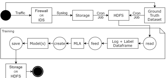
Thus, the motivation for this thesis was to deploy a system which is able to capture a large quantity of traffic that is perfectly cataloged as attack or non-attack in a ground-truth dataset, and store both this dataset and the logs generated by said traffic into a Hadoop Distributed File System. Afterwards, it reads all this data and feeds it to one or multiple Pyspark Machine Learning Algorithms (MLA) that create classification models able to distinguish attack traffic from regular traffic. These models are then saved so that they can be integrated into a network attack prediction or prevention environment.

The diagram in Figure1.1helps to visualize this concept solution.

Figure 1.1: Diagram of the solution concept.

1.3 Contribution

Not much of the available research brings together the application of machine learning techniques in a Big Data context for traffic log analysis. As such, this work contributes with:

• A system that can capture log files from a Firewall or an Intrusion Detection System and store them into a Hadoop Distributed File System cluster;

• A Pyspark application that can learn to classify incoming traffic by analysing large quantities of data stored by the log capturing system;

• The integration of four machine learning algorithms in the Pyspark application and an ex-ample of how they can be used to distinguish Distributed Denial of Service Attacks from regular normal traffic.

(19)

1.4 Dissertation Structure 3

1.4 Dissertation Structure

This work is organized into six chapters that guide the reader through the process of the concep-tualization, execution and completion of the proposed solution:

• Chapter 2- Technological Background: gives a concise explanation of the underlying subjects —Security Systems, Data Analytics, and Denial of Service Attacks;

• Chapter 3- State of the Art: presents the iterative process of the problem definition by reviewing the literature that focused this proposition;

• Chapter 4- Scalable Intrusion Detection: explains how the system was implemented, the challenges faced along the way, and what was done to circumvent them;

• Chapter 5- Methodology and Results: describes the dataset used and the results obtained with the algorithms used;

• Chapter 6- Conclusions: discusses the objectives accomplished and what could be done in future works.

(20)

(21)

Chapter 2

Technological Background

Given that this paper covers a wide range of subjects, this chapter will briefly review the main concepts present in this work: Firewalls, Intrusion Detection Systems, Data Analytics and Denial of Service attacks.

2.1 Firewalls

Firewalls were one of the earliest security concepts designed to protect systems and networks from external threats. They exist at the boundary of two networks to control the network traffic flow between senders and receivers with different security postures towards different kinds of traffic. [2]

In the early days, firewalls would only protect incoming lower layers of network traffic into the network, and not the traffic in between the network it protected. And, of course, it also wasn’t able to recognize all forms of attacks. Thus, as time went by, firewalls evolved to include some functionalities at other locations within the network and threats progressively moved from lower network layers to the application layer, which then reduced firewall effectiveness. [2]

Today, several types of firewalls exist that provide different services - however they most certainly contain one or more of these essential functions:

• Traffic redirection and IP address preservation: similarly to routers, some firewalls can forward traffic through the use of ipchains or iptables to allow different networks to com-municate. Even so, they don’t necessarily provide Network Address Translation (NAT). • Network distinction: the whole idea behind a firewall is to isolate a network from another,

so it can serve as a boundary even between same company networks.

• Protection against Denial of Service, Port Scanning and sniffing attacks: since firewalls act as a single point monitor of incoming and outgoing traffic it is possible to limit very specific traffic.

(22)

6 Technological Background

• IP and port filtration: the same way traffic can be forwarded, if a network manager deems certain sources or destinations untrustworthy, firewalls allow for IP addresses and ports to be blocked.

• Content filtration: proxy-oriented firewalls can be configured to identify and block content that a network manager considers harmful.

• Packet redirection: if for some reason there’s too much traffic going to a specific port, it is possible for a firewall to redirect some of that traffic to a separate host and forward said traffic.

• Enhanced encryption and authentication: firewalls are able to authenticate users and encrypt transmissions to firewalls on another network.

• Supplemented logging: it is possible to set up a firewall to record logs with information about the network packets that go through it, which can be later used to learn about port scans and various connections to the network.

2.1.1 Types of Firewalls

Before understanding the different types of firewall, it is important to remember the Open Systems Interconnect (OSI) model in order to have a comparison on how they operate (see Figure2.1).

Figure 2.1: OSI Model.

2.1.1.1 Packet Filtering

A packet filtering firewall works at the Network and Transport layers, where it makes decisions on whether to forward or block a packet based solely on the information of its source and destination IP and port or based on its protocol type; be it Transmission Control Protocol (TCP), User Data-gram Packet (UDP), Internet Control Message Protocol (ICMP), and so on. As such, in a way, a packet filter works similarly to a router. [3]

(23)

2.1 Firewalls 7

It is important to note that it can only handle individual packets and it is not able to keep track of TCP sessions. This means that spoofed packets coming through an outside interface pretending to be part of an existing session won’t be easily detected. [3]

The main reason to use this type of firewall is the filtering speed, even if it is not that difficult to spoof. Without having to inspect application data, packet filtration is almost as fast as a router but with the improved functionality of packet filtering. [3]

2.1.1.2 Stateful Inspection

To improve the security capability when dealing with network sessions, a stateful inspection fire-wall keeps a connection table with entries for each session that is being currently carried out. These entries are checked for the next packets and are automatically timed out after some customizable timeout period. [3]

When the firewall recognizes a first Synchronize (SYN) packet that initiates a TCP session, it creates a new entry so that the following Acknowledge (ACK) flags can be legitimized by matching the same entry. This way, it is possible for these firewalls to keep track of network sessions. [3]

For UDP communication, since it was designed with no concept of state, only a pseudo stateful inspection can be applied. Case in point, upon receiving the first UDP packet, the firewall creates an entry in the connection table so that the subsequent packets can be trusted into the network. [3] Moving up to the application layer, more stateful protocols can be found such as the File Transfer Protocol (FTP). Considering FTP is implemented so that when a user requests a file transfer to port 21 and the file is then sent back through port 20, the firewall must keep track of the initial established connection. Otherwise, it will not allow data to connect back in. Newer multimedia protocols such as RealAudio and NetMeeting share this same concept with FTP. [3]

Even though they are sometimes less secure than application proxies, the connection speed and protocol flexibility of stateful inspection firewalls make a strong argument for their continued use in current times. [3]

2.1.1.3 Application Proxy

To determine if a connection is allowed through, application proxy firewalls analyze packets all the way to the application layer - meaning that they have a better understanding of the information being transmitted, be it FTP, HyperText Transfer Protocol (HTTP) or any other. When sending messages from the internal network to the exterior, the firewall disguises the sender and acts as a proxy for the receiver. [3]

This way, addresses are hidden and the risk of message interception is greatly reduced - as such, a much better level of security is achieved at the cost of transparency and performance, as additional processing is required. However, newer models mitigate some of these issues. [3]

The downside of using such a firewall is that for each protocol it is necessary to have a corre-sponding proxy, which means that if a new application protocol is created, then a new correspond-ing proxy must be implemented as well. One way to go around this issue, but in a less secure way,

(24)

is to configure some generic proxies for IP, TCP, and UDP so that these can allow newer protocols through. [3]

2.1.2 Firewall Rules

To decide on whether or not to let a communication through, a firewall relies on a ruleset - which can refer to all the rules, or just the group of rules within a specific context. Generally speaking, most of the rules in the firewall evaluate connections on a first match basis. This means that when a connection comes through, the first rule that it can be applied to takes an action. If not a single rule was matched, traffic is generally denied. [4]

In addition to a ruleset, some stateful inspection firewalls may also have a State Table to remember connection information so reply traffic can be allowed automatically. The connection information in the table includes the source, destination, protocol, ports, and more information to guarantee connections are uniquely identifiable. To prevent memory overload, this table has a reconfigurable maximum size. [4]

With this mechanism in place, the firewall only needs to check the rules on the traffic’s first connection. Then, if it matches a pass rule, the firewall will create an entry in the state table and replay traffic of the same connection will automatically be allowed through by matching the table. This also includes related traffic using a different protocol (i.e ICMP messages in response to TCP or UDP). [4]

Firewall rules can disallow traffic in two ways: Block and Reject. Blocking is when no re-sponse is given to incoming traffic and is simply dropped. This is usually the default behaviour when denying communications. On the other hand, rejecting does send a response to let the sender know that the connection was refused. [4]

Rules can be based on multiple traffic characteristics to be filtered - the most important ones are:

• IP addresses: even if some firewalls cannot handle IPv6 traffic, all of them can filtrate traffic to and from certain IPv4 addresses.

• Protocols: a firewall might want to treat TCP, UDP, ICMP, IPsec, and many other protocols differently.

• Applications: specifically, application proxies can choose to block inbound or outbound traffic based on IP addresses and application level protocols (like HTTP) respectively. • User identity: some firewall technologies that make use of IPSsec VPNs (Virtual Private

Networks), Secure Sockets Layer VPNs, or Network Access Control (NAC) are able to enforce policies based no user identity.

• Network activity: time and periodicity of a connection can also be a rule of access for some firewalls.

(25)

2.2 Intrusion Detection Systems 9

2.1.3 Firewall Logs

Once the firewall decides what to do with the received traffic, it records all these decisions in the form of logs. It is important to note that logging is a critical part of maintaining the security of a network. Not only those logs can be used to ensure proper security configurations are set, but can also provide essential information about previous security incidents. [2]

The contents of a log file are usually: a timestamp of the actual time the event was logged, the hostname of the firewall that logged the event, and all the relevant event data which vary by protocol. Common fields for event data are:

• Rule number that identifies which rule was applied; • Reason for the log entry;

• Action taken that resulted in the entry log; • Traffic direction, in or out;

• IP version 6 or 4;

• And even more specific information like protocol, flags, anchor, real interface, etc.

2.2 Intrusion Detection Systems

As Internet usage grew, so did the threat of attacks, leading to the creation of various new ways to try to prevent and protect from such incidents. One of these ways was through the implementation of Intrusion Detection Systems. [5]

A generic IDS gathers intelligence from the system it wants to protect so it can perform di-agnosis on its security status. This way, it may be able to discover security breaches, previously attempted breaches or vulnerabilities that, if unattended, could potentially lead to breaches. [5]

In a broad scope, an IDS can be described as a detector that surveys information to be pro-tected. Besides detecting, some IDS’s may also be able to launch probes that trigger an audit process, for example, requests an application’s version numbers. Then, if some sort of threat is identified, a countermeasure may be taken to either prevent malicious action from being executed or to return the system back to a secure state. [5]

To accomplish its designed duties, an IDS uses three different types of information: long-term information about the techniques used in intrusion detecting, information about the current state of the system and descriptive information of the events that are happening on the system. [6]

Debar [6] suggests three ways to classify an IDS: by the detection method, the audit source location and the detection paradigm.

The detection method can be through the analysis of the monitored system’s behaviour, or through the analysis of information about the attacks.

(26)

Intrusion Detection Systems can also inspect different sources of input. For instance, this input information can be the host system logs, application logs, network packets, or even alerts generated by other Intrusion Detection Systems. [6]

The detection paradigm refers to the evaluation done by the IDS, which can be about the system state (secure or insecure) or its transitions (from secure to insecure). In either case, this evaluation can be performed with or without stimulating the system and obtaining a response. [6] Furthermore, the action taken once an attack is detected can be actively reacting to it by cor-recting an insecure state, proactively reacting by logging out possible attackers or closing down services, or just passively generating alarms. [6]

2.3 Data Analytics

With the recent advancements in data processing, storage and transmission, data analysis has be-come one of the fastest growing markets in the world. So much so, that it even came to affect our day-to-day lives within our internet habits. It is almost impossible to open a website without being prompted with a data collection policy warning. There are many fields that can benefit from knowledge extraction: agriculture, education, environment, industry, medicine, and many other scientific disciplines. [7]

Once we understand the goal of data analysis is to collect and transform large amounts of incomprehensible data into valid, useful, and human-understandable information, we can see the potential to support work, reduce waste, increase product value and much more. [7]

However, before results can be achieved there is a process to be followed. First, data needs to be collected, then organized, then either or both pre-processed and transformed, and finally modeled. In this final step, it is possible to model the data in two ways: it can be classified with the intent of achieving a better description, or it can be modeled to predict the outcome of future similar event - but, of course, before using data for a predictive task it is most helpful to describe it first. [7]

2.3.1 Descriptive Analytics

Suppose some data is collected in the form of a table with multiple columns where thousands of entries were recorded. Looking through all that information and trying to find a pattern would be a tremendous task to accomplish, not only in the exploratory part of the task but in the organizing part of the task. That is exactly what descriptive analytics aims to do: use methods that describe data by summarizing their characteristics or by visualizing the characteristics. [8]

There are three categories of data mining methods: univariate, which is for single attribute problems; bivariate, which is for problems with two attributes; and multivariate, which is for groups with more than two attributes. [8]

On descriptive univariate analysis, whether in a qualitative or quantitative scale, it is common to look at data according to its absolute or relative frequency; at various statistical characteristics

(27)

2.3 Data Analytics 11

like minimum, maximum, average, mode, and median; and to try to find a matching probability distribution like the uniform distribution or the normal distribution. It’s also useful to use pie chars, bar charts, line charts, area charts, and histograms to help visualize the data. [8]

Descriptive bivariate analysis is trickier since the attributes can be in different qualitative or quantitative scales. As such, frequency statistics alone may not be good enough to describe data. Even so, when there is no such issue, some of the most used techniques are scatter plots, co-variance, Pearson correlation, and Spearman’s rank correlation (except when both attributes are ordinal). When there’s at least one nominal qualitative attribute, contingency tables facilitate data visualization. [9]

Descriptive multivariate analysis is always treated as multiple univariate or bivariate analysis problems put together. Therefore, a combination of the previously mentioned methods are used in this case. [9]

Although these methods already provide a good quantity of information, there’s more interest-ing analysis that can still be done by partitioninterest-ing the data into groups. This is done by clusterinterest-ing techniques and, given that they only use predictive attributes, they’re considered unsupervised techniques. [9]

The most commonly used clustering algorithms are K-means, Density-based spatial clustering of applications with noise(or DBSCAN, for short) and Agglomerative Hierarchical Clustering. Despite being the most computationally efficient of the three, K-means is also less robust against noise and outliers. [8]

Another way to describe data is to do frequent pattern mining that, as the name suggests, attempts to find repeated and recurring features within the data set designated for description. This can be done in three different ways, by looking for:

• a combination of items that appear together in different instances, referred to as frequent itemset mining;

• interesting relations between different combination of items, referred to as association rule mining;

• frequent sequences of items not necessarily contiguous, referred to as frequent sequence mining.

2.3.2 Predictive Estimation

Besides descriptive analysis, prediction is also one of the subjects of study in the data analytics field. There are two main prediction tasks, namely regression and classification. Regardless of the kind of task, their objective is to label an unknown item by looking at its characteristics, having previously learned the labels of known items also by looking at their characteristics. [8]

What differentiates the two tasks is the learning methods they use and the type of labeling they aim to do. [8]

(28)

As a matter of fact, regression tasks are used to find models or functions that best describe data into continuous real values. The most used techniques for this task are: multivariate linear regression, ridge regression, least absolute shrinkage and selection operator, principal compo-nents regression, partial least squares, and multivariate adaptive regression splines. [8]

Once a model is crafted, it is important to make sure it is going to predict correctly as much as possible. One of the simplest ways to do so is to divide the data set into a training set and a test set. To do so, there are several partition methods like random sub-sampling, k-fold cross-validation, leave-one-out, and bootstrap. [8]

A classification task is different in the way that it separates the data into multiple, discrete value, categorical classes. The most used techniques for this task are: logistic regression, Naïve Bayes, and AdaBoost. [8]

More complex tasks that don’t simply fall into regression or classification categories due to the nature of their data have different requirements. For those cases, more complex algorithms like k-nearest neighbors, decision tree induction, model tree induction, artificial neural networks, ran-dom forest, bagging, support vector machines, or deep learning (convolutional neural networks) are used. [8]

2.3.3 Big Data

The term Big Data came to be when the volume of data collected, its complexity and the processing required to analyse it became too grand to be achieved by the usual methods of data analytics. Since then, it turned into its own issue within the data science community. [8]

The solution found was to create computer clusters that combine into a distributed system not only to store a vast amount of data but to process it. To tackle software limitations, the MapReduce implementation was developed to aid the processing task. [8]

But this only works if the solution follows the same principles as a distributed system. It must guarantee that:

• if a computer fails during a processing task, another computer must assume it;

• if a computer fails, all the data it had must be duplicated somewhere else in the cluster; • when a computer recovers from a failure, it must be able to return to the cluster again; • it must be easy to remove or add computers as the processing requirements change; • the distributed system must look like a single system to the data analyst.

2.4 Distributed Denial of Service attacks

A Denial of Service (DoS) attack is an attempt to overload a specific network resource with fake traffic so that it becomes unable to answer all (if any) connections from legitimate users. And as

(29)

2.4 Distributed Denial of Service attacks 13

the name suggests, a Distributed DoS (DDoS) attack is deployed by multiple attacking entities. [10]

What makes DDoS attacks possible is how the current Internet was designed. For instance, the focus is placed on moving packets as effectively as possible by providing a minimalist yet best-effort packet forwarding service in the intermediate network. That, in turn, tasks the sender and receiver with the responsibility of implementing a reliable, secure and robust protocol. This way, the packet forwarding provided by the intermediate network can stay simple and optimized. Given both parties are in charge of their communication security, were one of them to conduct themselves in a malicious manner without the other realizing, the result would be at the hands of the perpetrator. [11]

Considering network components have limited resources, it is never impossible to flood a host, network or service with too many users for it to process. [11]

Attackers also usually sabotage insecure systems to launch their attacks on top of spoofing their own IP. This makes accountability really difficult to enforce, as Internet management is distributed and there can be many different kinds of local policies for each network set by their owners. [12]

The idea behind these attacks is to inflict some sort damage on the victim —whether for revenge, prestige, material gain, or even political reasons. Thus, banks, e-commerce websites, corporate networks, news websites, and governmental websites are common services that become victims of these kind of attacks. [12]

(30)

(31)

Chapter 3

State of the Art

Leading up to this work, the scope of the project wasn’t entirely defined. However, from the start, it was deemed fundamental to combine the concepts of Firewalls, Data Analytics, Big Data and Machine Learning, in an attempt to aid the protection of a system by detecting incoming malicious traffic.

This chapter therefore aims to review the literature that helped narrow down the characteristics of this assignment into its conclusion. From here, the first step was to look into how data mining and data analytics is being used to detect or distinguish malicious traffic from regular traffic in firewall studies.

3.1 Firewall log analysis and rule inference

Golnabi et al. [13], for example, used data mining to analyse LINUXfirewall logs as a way to obtain information about the effectiveness of the firewall’s own rules. If the examination showed that some rules were not working as intended or that some violations were occurring, then some information might be gathered and used to update or remove those rules.

What is particularly interesting about their work is that they chose to transform the firewall logs into “primitive rules” with their own algorithm (Mining firewall Log using Frequency - MLF) that deduces a rule from the log’s information. They did not specify, however, if they used a real dataset or if they created artificial traffic to generate those logs.

They then used an aggregation algorithm they developed (FilteringRule Generalization -FRG) to read all the rules deduced from MLF and try to combine them into as few rules as practi-cable, while at the same time detecting possible rule conflicts and anomalies.

Despite not using any machine learning algorithms, not experimenting with distributed storage systems, and taking a different approach on how to encounter malicious traffic; Golnabi et al. still used firewall log analysis in an interesting way that validates the usefulness of using data mining within this scope.

(32)

16 State of the Art

On the same line of thought, Breier and Branišová [14] also induced rules, but for an Intrusion Detection System, from the logs this system recorded in the 1998 DARPA Intrusion Detection Evaluation Set, and from Snort logs that could confirm if an attack was made or not.

They developed two anomaly detection algorithms, one being implemented in the Java pro-gramming language, and the other Hadoop-based, implemented with its MapReduce method. The log files were also stored in a Hadoop Distributed File System (HDFS).

In these supervised learning algorithms, they claim to have used a combined classification and clustering effort to detect outliers that may reveal an attack. Unfortunately, references to the details of their implementation, or even the features extracted to achieve their results were not found. From here, they created the rules.

To evaluate the success rate at which attacks were identified, they divided the data into a train-ing set and a test set so they could compute True Positive, False Positive, and Error rates. Finally, they compared the processing speed of their algorithms with Apriori and FP-growth, claiming to have achieved competitive results with the Hadoop-based one.

3.2 Firewall rule efficiency analysis through log mining

Moving away from rule inference, Ucar and Ozhan [15] analysed Windows firewall logs to eval-uate if the firewall rules were working properly. Thus, they used anomaly detection not to find malicious traffic, but traffic that did not follow the firewall rules.

Their method relied on the distributed computing system WEKA running six machine learning classification algorithms —Naïve Bayes, kNN, Decision Table, HyperPipes, OneR, and ZeroR, all supervised learning algorithms— to assess how rules behaved according to the traffic recorded in the log files.

From what was perceptible, they extracted nearly 5 million logs of real traffic that passed through a firewall. The features extracted from the logs were the policy, protocol, ports, IPs, packet information, connection table entry, and few more.

The algorithm classification performance was evaluated with Kappa-Coefficient Statistics, F-Measure, and Root Mean Squared Error. They came to the conclusion that kNN yielded the best results.

Gutierrez et al. [16] combined visual and statistical methods and integrated them into an analytical application that assisted in the firewall log analysis process.

To develop such framework, they implemented an automated Tabulated Vector Approach (TVA) to handle log files, so that they could use the Mahalanobis distance (MD) to identify anoma-lies by relative magnitudes. They also proposed the usage of a “breakdown distance” (BD) as an alternative to MD.

The TVA is a way to build a multivariate dataset containing only numeric values by extracting features from the log files that contain non-numeric information, like protocols, IP addresses, firewall actions performed, etc.

(33)

3.3 Malicious traffic detection through firewall log analysis 17

The dataset built by TVA condensed all that information into variables like: number of times an IP wasn’t able to be accessed, number of times a specific IP connected to another specific IP, how many different IPs tried to access a designated IP, among others. After data had been processed, they generated heatmaps, histogram matrices, and network graphs to aid an analyst to inspect the firewall traffic and identify potential security breaches and attacks.

3.3 Malicious traffic detection through firewall log analysis

Ertam and Kaya [17] looked to classify the action the firewall should take on traffic —these actions being “allow”, “deny”, “drop”, and “reset-both”— according to its features. This means they did not try to find malicious traffic among the logs, they simply tried to predict what action the firewall would take without looking at the rules. Why they felt this was important is not specified within their writing, it was simply mentioned as preparation for a future work they are designing.

As means of prediction they decided to use a supervised learning technique, multiclass Support Vector Machine (SVM), with linear, polynomial, sigmoid, and Radial Basis Function functions that separated the traffic into the actions that the algorithm thinks the firewall should take on them. The features which helped make the decision were the ports, bytes, packets, and time.

Overall, they classified over thirty thousand logs from real traffic that went through a Palo Alto 5020 Firewall at their department and evaluated the classification process with precision, recall and F1 Score along with receiver operating characteristic curve (ROC curve, for short).

Dietz and Pernul [18] also utilized statistical methods to uncover anomalies in firewall event logs, in real-time, in a Big Data distributed system structure. They accomplished this by imple-menting a tool in Java with the Apache Flink stream processing system.

The streamed data was provided by the case study of the DINGfest project, with which they tested their proposed stream anomaly detection technique. This case study contains a log stream of real-world security events that can be simulated to produce data instances over time.

The point of their study was not to discuss better ways to capture malicious traffic, but how to determine the baseline of what constitutes normal traffic and how to continuously compute the arithmetic mean and standard deviation as more data flows in. As such, they did not discuss different anomaly algorithms, nor what features were used in the data mining process.

At this point, after going through some literature, the plan devised for this thesis was to create a network, install a firewall to protect it, perform attacks to that network amidst regular generated traffic and capture enough log data for analysis with machine learning algorithms.

However, major world events prevented some of these ideas to come to fruition. Consequently, the plan needed to be adapted considering the new requirement of moving to a remote work con-dition.

Given the circumstances, it was decided that the project would be split into a virtual log cap-turing prototype and a log data analyser that could detect DDoS attacks on a scalable environment. This way, the core idea could stay similar enough to the initial design.

(34)

18 State of the Art

3.4 Detecting DDoS attacks with Machine Learning

Gupta [19] aimed to create a DDoS detection mechanism focusing on feature selection algorithms that could sort features by their importance. In fulfilling this task, a dataset from Knowledge Discover Dataset Cup 1999was used, in which there are forty-one different categories of data.

To sort features from most to least important the algorithms used were Information Gain, Chi-Squared, and Recursive Feature Elimination (RFE), ending with the employment of a novel Weighted Ranked Feature Selection (WRFS), to create a final list of features sorted by their weighted ranks attributed by the previous three algorithms.

Afterwards, each sorted feature was incrementally fed to four classification algorithms — Naïve Bayes, Support Vector Machines, Decision Tree, and Random Forest— in different runs. Accuracy, precision and recall were the measures used to evaluate the classification process. The best performing of the four was held to be Random Forest with 99.83% accuracy and more than 99% of precision and recall.

To finish, real-time network traffic was captured in a simulated test-bed and used to appraise the models created. All experiments were done in a Virtual Private Network (VPN) environment to prevent attack packets from spreading into other targets unintentionally. In these trials, while using a fraction of the attributes from the network packet, the proposed model claimed to detect the simulated DDoS attacks with roughly 99.8% accuracy.

Even though Gupta only did binary classification and did not develop a detection system for a Big Data scenario, the methodology was quite similar to the one being planned for our thesis.

Patil et al. [20] proposed a victim-end system to detect DDoS attacks on a scalable environ-ment. Legitimate and attack traffic was captured using the Wireshark network traffic sniffer tool and then stored on a Hadoop Distributed File System. However, the detection was done with mapper and reducer jobs instead of Machine Learning algorithms.

First, Yet Another Resource Allocator (YARN) assigned datanodes to perform the detection, on which the mapper would task the extraction of source and destination IPs, the protocol used, number of packets, delta time, and time window with which it computed the entropy using the Shannon Entropy equation. Then the reducer compared this entropy with a threshold interval from which, if it fell outside of, the according traffic flow was considered a DDoS attack. This threshold interval was computed with the entropy’s mean, its standard deviation, and a tolerance factor.

They validated this model using real datasets (MIT Lincoln LLDDoS1.0, CAIDA) and live traffic generated with their network testbed configuration. Even if the dataset wasn’t particularly big and the computation of the threshold appeared to be slightly arbitrary, the structure surrounding it is a Big Data setting and they reported to have a detection rate of 97% .

3.5 Summary

With the papers described in this chapter, we come to the conclusion that even though much work has been done around Firewalls, Intrusion Detection Systems, Big Data, and Machine Learning,

(35)

3.5 Summary 19

we have yet to find a paper that uses all the concepts we have been discussing so far. Although we did find projects that are near to our concept, they seem to be constantly missing at least one component, be it not having Big Data in mind, not using solely logs, not using proper anomaly detection algorithms, or not using machine learning algorithms the way we pretend to.

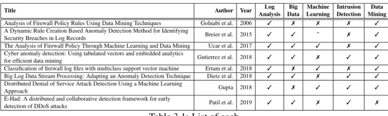
Title Author Year Log Big Machine Intrusion Data

Analysis Data Learning Detection Mining Analysis of Firewall Policy Rules Using Data Mining Techniques Golnabi et al. 2006 3 7 7 7 3 A Dynamic Rule Creation Based Anomaly Detection Method for Identifying

Breier et al. 2015 3 3 ˜ 7 3 Security Breaches in Log Records

The Analysis of Firewall Policy Through Machine Learning and Data Mining Ucar et al. 2017 3 3 3 7 3 Cyber anomaly detection: Using tabulated vectors and embedded analytics

Gutierrez et al. 2018 3 3 7 3 3 for efficient data mining

Classification of firewall log files with multiclass support vector machine Ertam et al. 2018 3 7 3 7 3 Big Log Data Stream Processing: Adapting an Anomaly Detection Technique Dietz et al. 2018 3 3 7 3 3 Distributed Denial of Service Attack Detection Using a Machine Learning

Gupta 2018 3 7 3 3 3

Approach

E-Had: A distributed and collaborative detection framework for early

Patil et al. 2019 3 3 7 3 7 detection of DDoS attacks

Table 3.1: List of each.

As this chapter comes to a conclusion, it is important to mention that much more literature was consulted than what was outlined here. Most of it was not included due to similarities between each other and to include them all being this identical would seem repetitive. So, ultimately, the ones that were kept were the ones that could better represent how the idea evolved through the course of the project.

The solution proposed in this work is an application capable of generating Pyspark Machine Learning models able to distinguish attack traffic from regular traffic, by analysing large quantities of captured log data (with no feature extraction), that are classified with a certain ground truth dataset —all executed in a distributed environment.

(36)

(37)

Chapter 4

Scalable Intrusion Detection

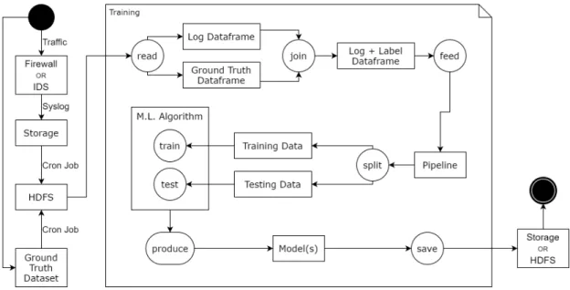
As stated in section3.5, the tool proposed in this work requires a firewall or IDS to be the target of attack and regular traffic so that logs can be captured and cross-referenced with a ground-truth dataset. Then, as can be seen on Figure 4.1, all this information is read onto a log dataframe and ground truth dataframe, these are merged into a single one that takes the log features and the ground truth label. A pipeline formats the merged dataframe, before splitting it and feeding it to one or more Machine Learning Algorithms that create classification models. Finally, this model is saved for future use in classifying logs or incoming traffic.

Figure 4.1: Full Application Diagram.

4.1 IDS log Capturing

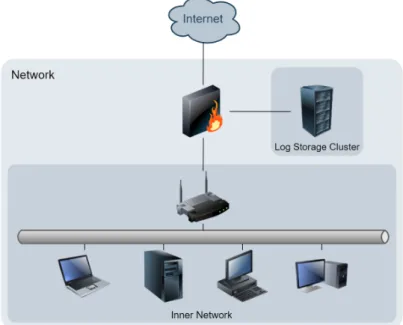
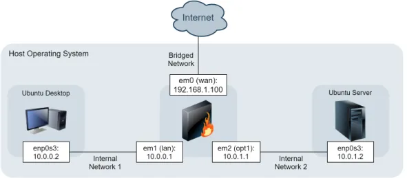
Before setting up a log capturing routine, it was necessary to design a network architecture that looked credible from a realistic standpoint (Figure4.2). Of course, this configuration was to be virtualized into a simpler test environment condition.

(38)

22 Scalable Intrusion Detection

With that in mind, the inner network in Figure 4.2 can be represented by a single virtual machine for simplification reasons. The log storage servers can also be virtualized as docker images running on a single virtual machine image to simplify the implementation.

Figure 4.2: Conceptualization of a simple realistic protected network.

Consequently, the machines chosen for virtualization were a PfSense firewall [21], to capture traffic and generate logs for future analysis; a Ubuntu [22] server to run Docker [23] environments that will simulate an HDFS cluster [24] to store the logs captured by the firewall, and run Pyspark [25] machine learning algorithms; and a Ubuntu desktop from which the firewall could be managed and serve as the representation of an inner network where a company might have their web servers, data servers, production computers, etc.

All virtual machines were virtualized using Oracle VM VirtualBox Manager [26]. The full non-default configuration details of the three virtual machines implemented can be consulted at Table4.1.

Setting PfSense Firewall HDFS & Spark Cluster Ubuntu Desktop Operating System FreeBSD (64-bit) Ubuntu (64-bit) Ubuntu (64-bit)

Base Memory 521 MB 4096 MB 1024 MB Storage 6 GB 20 GB 10 GB

Network 1 Bridged Adapter 1 Internal Network Adapter 1 Internal Network Adapter 2 Internal Network Adapters

Table 4.1: Virtual machine settings for each image.

With the three images installed and with all the settings in place, the next step was to configure PfSense network interface’s IPs and Dynamic Host Configuration Protocol (DHCP) servers (see Figure4.3). Once done, the Network Adress Translation (NAT) table rules were set so that the virtual machines could reach each other and the internet.

(39)

4.1 IDS log Capturing 23

Then, Suricata [27] package was installed and enabled on the firewall with all the default settings to listen to WAN —except for the Eve JavaScript Object Notation (JSON) Log setting, which was set to output the logs onto a syslog server created on the Ubuntu Server virtual machine. Once syslog server was receiving the logs, it was time to set up the a Hadoop File system to store all of them. As such, it was wise to look for docker images online that had both Pyspark and HDFS implemented. After finding multiple candidates, the chosen one ended up being /singular-ities/spark[28] that, despite not having Apache Spark updated to the latest version, it was still the lightest and simplest implementation that fulfilled the requirements.

Figure 4.3: Conceptualization of a network.

To make node scaling more straightforward to deploy, the docker images were described using a docker-compose file, in which the master node was defined to be created with a shared volume, and worker nodes were defined to have one dedicated Central Processing Unit (CPU) core and 2 GB of Random Access Memory (RAM). For experimentation purposes, one master node and three worker nodes were deployed.

Finally, to transfer the Eve JSON logs from the Ubuntu Server virtual machine into the Hadoop Distributed File System provided by the docker images, cron [29] jobs were implemented. Cron is a Unix software utility which allows users to schedule jobs at fixed times, dates or intervals. With this tool, log transfers were achieved with timed shell scripts.

In total, two crontab jobs were put into action: one within the Ubuntu server, with two scripts with instructions to move the logs onto the docker shared volume, and to delete these logs a few moments later to save space; and the other in the master node docker image to copy the logs from the shared volume into the HDFS. Note that enough time was given to transfer the logs onto the shared volume and to then transfer them from the shared volume into the HDFS, without deleting them first.

And with that, the log capturing prototype was functioning and proved to be feasible to deploy on real hardware. Unfortunately, it was at this point that the Coronavirus Disease 2019 (COVID-19) forced many facilities to temporarily shut-down, including our University. Without access to

(40)

University labs, it was not possible to arrange an actual hardware configuration to execute different cyber-attacks on. Thus, that plan had to be discarded.

Since the log capturing was functional, it was then reasonable to assume that running Suri-cata in offline mode with PCAP files simulating traffic would produce the same log results. Upon considering different possibilities, it was decided that the 2019 DDoS Evaluation Dataset (CICD-DoS2019) from the Canadian Institute for Cybersecurity [30] would be used because has recorded different types of DDoS attacks amidst regular traffic. And not only does it have a substantial amount of PCAP data, but also provides their respective categorization with a dataset to establish the ground truth with.

4.2 Ground truth collection for training

Considering that one of our objectives was to analyse our own logs as if we had generated the traffic and captured it with the prototype from the previous section, the extracted statistical features computed by Sharafaldin et al. [31] were discarded in favour of the Eve JSON logs characteristics to be obtained by running Suricata in offline mode with the PCAP files.

To create the ground truth table with the log fields and its correct label, both batches of log files and CICDDoS2019 were read into Pyspark dataframes to be cross-referenced according to their respective timestamps, source and destination IPs and ports. This way, it was only necessary to add a new column to the log dataframe.

To note that, due to divergent timestamp formats and a 4-hour shift between the labeled dataset and the logs, some simple operations were necessary to make both tables’ values comparable. The code snippet of the table merging operation can be seen in Listing 4.1, where it is possible to understand that the list cond contains all the conditions that need to be met for each entry to be selected. This process also filters out erroneous entries without all these required fields.

1 cond = [grndTr_df.timestamp_rest == logs_df.timestamp_rest,

2 grndTr_df.timestamp_h == logs_df.timestamp_h, 3 grndTr_df.Source_IP == logs_df.src_ip, 4 grndTr_df.Source_Port == logs_df.src_port, 5 grndTr_df.Destination_IP == logs_df.dest_ip, 6 grndTr_df.Destination_Port == logs_df.dest_port] 7

8 merged_df = logs_df.join(grndTr_df, cond).select(logs_df["*"],grndTr_df["Label"]). drop("flow_start", "timestamp_rest", "tls_notafter", "tls_notbefore", ... ) 9 merged_df = merged_df.select(’*’, col(’Label’).alias(’label_idx’)).drop("Label")

Listing 4.1: The code snippet where the logs and ground truth dataframes are merged

4.3 Log features used for classification

Because some logs attributes returned by the PCAP files showed multiple empty fields, some scrutiny was required in investigating which features should be dropped and which should be

(41)

4.3 Log features used for classification 25

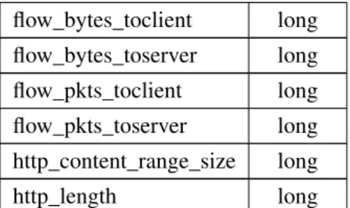
chosen. However, from the 138 different fields observed, various categorical fields with too many or too similar categories, and numerical fields with small interval values were then mindfully discarded; e.g. log timestamp, source and destination IPs, source and destination ports, flow identificator, to name a few. The features that ended up being selected were the ones listed on Table4.2. The full log format can be consulted at Suricata’s documentation [32] web page.

Feature Type categorical features alert_action string alert_category string alert_severity long alert_signature_id long app_proto string event_type string flow_reason string flow_state string flow_alerted boolean http_content_type string http_method string http_user_agent string http_status long proto string tcp_state boolean tcp_flags boolean tcp_flags_tc boolean tcp_flags_ts boolean tcp_ack boolean tcp_fin boolean tcp_psh boolean tcp_rst boolean tcp_syn boolean tls_session_resumed boolean tls_fingerprint string tls_issuerdn string tls_serial string tls_sni string tls_subject string numeric features flow_age long

(42)

26 Scalable Intrusion Detection flow_bytes_toclient long flow_bytes_toserver long flow_pkts_toclient long flow_pkts_toserver long http_content_range_size long http_length long Table 4.2: Features selected from the log files.

Another objective of ours was to use little to no feature engineering, with the intention of treating each entry like an incoming package that had just reached the Firewall/IDS, and like the model would decide if the package should or not be dropped. This way, switching to different PCAP files and a corresponding labeled dataset would require minimal, if any, change to join and create a different ground-truth.

Also, considering the size of the dataset, generating more features would increase the running time of the experiments to perform. As such, it made no sense to generate features from the data.

4.4 Pipeline

Pyspark Machine Learning Algorithms take data in a very specific format: a vector column with all the feature data, and a column with the corresponding label. The Listing4.2was adapted from Databricks official website [33] and it shows how a pipeline is used to execute all these steps.

In the for cycle, each categorical feature is encoded into integers, as the algorithms don’t take strings as inputs. Same goes for the labels, which are assigned to 0 or 1 if it’s a binomial problem, or from 0 to n − 1 classes if it’s a polynomial problem. Then, all features (numerical and categorical) are joint together withVectorAssembler. Finally, with all these stages set to the pipeline, the merged dataframe is then fed to the pipeline so it creates the vector column and the label column.

1 for cat_col in categorical_features:

2 stringIndexer = StringIndexer(inputCol = cat_col, outputCol = cat_col + ’_index’) .setHandleInvalid("keep")

3 encoder = OneHotEncoder(inputCol = stringIndexer.getOutputCol(), outputCol= cat_col + "_class_vec")

4 stages += [stringIndexer, encoder]

5

6 label_string_idx = StringIndexer(inputCol = ’label_idx’, outputCol = ’label’) 7 stages += [label_string_idx]

8

9 assembler_inputs = [c + "_class_vec" for c in categorical_features] + numeric_features

10 assembler = VectorAssembler(inputCols = assembler_inputs, outputCol = "features") 11 stages += [assembler]

(43)

4.5 Classification Models 27

12 pipeline = Pipeline(stages = stages) 13 pipelineModel = pipeline.fit(merged_df)

14 merged_df = pipelineModel.transform(merged_df)

15 selectedCols = [’label’, ’features’] + categorical_features + numeric_features 16 merged_df = merged_df.select(selectedCols)

Listing 4.2: Code snippet of the data preparation process

4.5 Classification Models

Having the dataset ready for analysis, four algorithms were used to create models capable of distinguishing regular traffic from DDoS attacks: Logistic Regression, Naïve Bayes, Decision Tree, and Random Forest, which were fundamentally chosen because, from the ones provided by Pyspark, these supported multinomial classification, which gave us more options for experiments and result comparisons.

In the same thread, no cross validation was performed, given the large amount of data - doing so would considerably hinder performance, extending the time of each test run, which already lasted a considerable amount of time.

Since all the libraries and dataframes used in the classification task were from Pyspark, then everything was parallelized and distributed natively by Spark.

4.5.1 Logistic Regression

Logistic Regression (LR) is a probabilistic machine learning algorithm which estimates the prob-ability of an object fitting in a particular class given its features — as do all the algorithms in this category. To do so, the Bayes’ theorem is applied as shown in Equation4.1. [8]

P(y|X ) = P(X |y) × P(y)

P(X ) (4.1)

In this equation, X represents the vector of attributes defining an object, while y represents a classification label. Consequently, P(y|X ) designates the probability of class y being true when an object is defined by X attributes, while P(X |y) designates the probability of an object having X attributes when it is classified as y. [8]

LR is a member of the discriminative group of probabilistic algorithms. As such, it adjusts a logistic function to a training data set, which in turn generates a straight line dividing the objects into two classes. In contrast to the linear function, LR returns values in the [0, 1] interval. [8]

Firstly, logistic regression is applied to compute the odds of a specific object belonging to either of the two classes, which are values in the [0, 1] interval. The odds ratio for the two classes is then calculated and a logarithmic function is applied to the result. The end result is known as the log-odds, or logit. To find the discriminant function, linear regression can then be used. [8]

Thus, it is clear that using logistic regression induces a linear classifier, estimating of class probabilities using the line equation obtained by a discriminant function. [8]

(44)

Variable Name Setting Value

maxIter Number of max iterations 100

regParam Regularization parameter 0

elasticNetParam ElasticNet mixing parameter 0

tol Convergence tolerance 1.00E-06

fitIntercept Fit an intercept term TRUE standardization Standardize training features before fitting the model TRUE aggregationDepth Suggested depth for treeAggregate 2

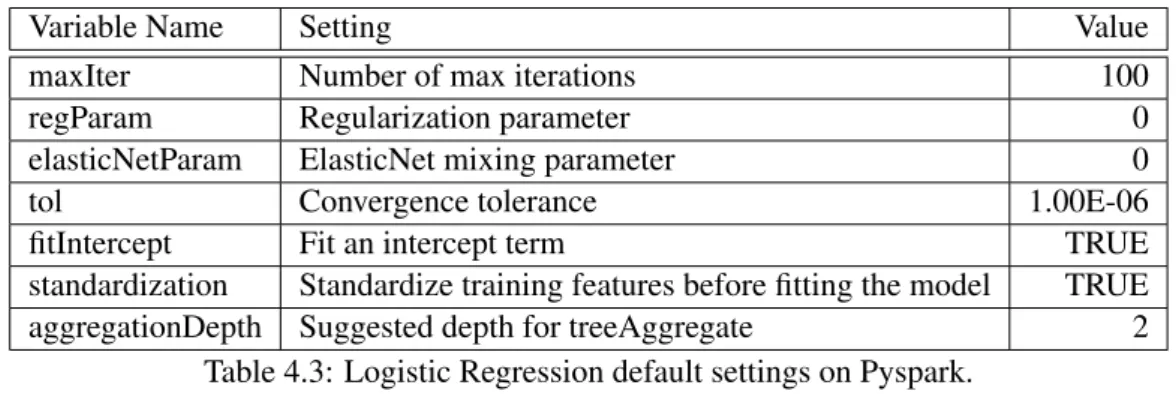
Table 4.3: Logistic Regression default settings on Pyspark.

While logistic regression returns a quantitative value —a probability—, it must then be trans-formed into a qualitative value —a class label. In binary problems, when such probability is less than 0.5 the negative class is predicted; otherwise the positive class is predicted. When used in multinomial problems, LR treats each class in a “one versus the rest” approach, the same manner it would treat a binary problem. [8]

The algorithm was run with its default Pyspark settings as seen on Table4.3.

4.5.2 Naïve Bayes

On the other category of probabilistic algorithms is Naïve Bayes (NB). As a generative classifi-cation algorithm, it induces models with emphasis on the probability of an object belonging to a specific class, by using the Bayes theorem defined by the previous Equation (4.1). This formula is then used to determine the probability that a certain object belongs to a specific class. In order to predict the class of a new object, if we have m classes, we must therefore use the Bayes theorem m times, one for each class. [8]

After analysing the data and determining the probability of an object being a part of each of the available classes, the class with the highest probability value is assigned to the object X . Thus, NB can be used in classification tasks with any number of classes. [8]

To use Bayes’ theorem the value of P(X |y) must be obtained. As previously mentioned, X stands for the vector of it’s objects features, so P(X |y) can defined by Equation4.2where x repre-sents each of the object’s features. [8]

P(y|X ) = P(x1|y) × P(x1|y) × ... × P(xn|y) (4.2)

On Pyspark, the only setting available, smoothing, was kept with its default value of 1.

4.5.3 Decision Tree

In order to apply a range of different models to test our sorted lists, we decided to include a Decision Tree (DT) classifier —-one of the most widely used algorithms in classification and regression problems. This algorithm creates a branched structure where each feature is represented

(45)

4.5 Classification Models 29

by a tree node, each decision (rule) is represented by a tree branch and each possible outcome is represented by a leaf —-thus making the algorithm easy to understand and interpret. [8]

While implementing a Decision Tree, a few key steps must be taken: 1. The best attribute should be selected and placed at the “root” of the tree;

2. The training dataset should be divided in subsets, so that each subset contains only data with the same value from a specific attribute;

3. Both steps 1 and 2 should be repeated until a “leaf node” is found for every “tree branch”. To predict the value of a class variable through this type of algorithm, the process should be started at the root of the tree and the values stored in the root should be compared with those of the instance’s attribute. Based on the obtained results, a branch should be chosen to follow until the following “tree node”. This process is then repeated until the final “leaf node” is reached and the predicted value of the class variable is found. [8]

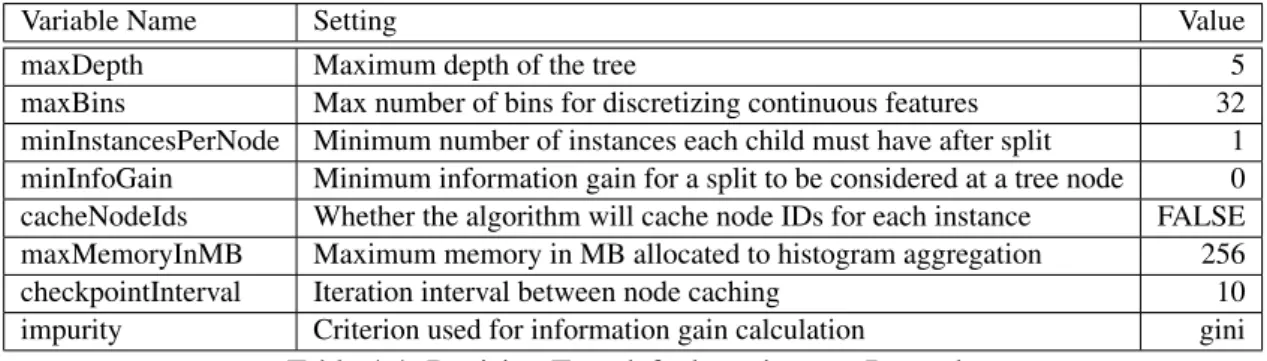
Decision Tree algorithm was also run with its default Pyspark settings, as seen on Table4.4.

maxDepth Maximum depth of the tree 5

maxBins Max number of bins for discretizing continuous features 32 minInstancesPerNode Minimum number of instances each child must have after split 1 minInfoGain Minimum information gain for a split to be considered at a tree node 0 cacheNodeIds Whether the algorithm will cache node IDs for each instance FALSE maxMemoryInMB Maximum memory in MB allocated to histogram aggregation 256 checkpointInterval Iteration interval between node caching 10 impurity Criterion used for information gain calculation gini

Table 4.4: Decision Tree default settings on Pyspark.

4.5.4 Random Forest

Another algorithm included in the classification process was Random Forest (RF). This method is, in essence, a compilation of multiple decision trees that work together and are trained using the bagging method —-which, in turn, is rooted in the concept that the effectiveness of any end model can be improved by the combination of several other models. Although in this study we use Random Forest for a classification problem, it can be used in regression as well. [8]

numTrees Number of trees to train 20

featureSubsetStrategy The number of features to consider for splits at each tree node auto subsamplingRate Fraction of the training data used for learning each decision tree 1

Table 4.5: Random Forest default settings on Pyspark.

Despite sharing most of the same hyper parameters as a Decision Tree, a Random Forest additionally has hyper parameters of a bagging classifier, which regulates the ensemble of “trees”

(46)

it encompasses. Rather than search for the best feature whilst splitting a node, a Random Forest searches for the best feature available in a random subset of features – thus creating a greater diversity and ultimately resulting in a better model. [8]

To keep uniformity with all algorithms, RF too was run with its default Pyspark settings. The hyper parameters shared with DT keep the same values as seen on Table4.4, the rest of the parameters are described on Table4.5.

(47)

Chapter 5

Methodology and Results

5.1 Dataset description

The CICDDoS2019 dataset imparted by the Canadian Institute for Cybersecurity is part of a study by Sharafaldin et al. [31] in which they propose a taxonomy for DDoS attacks, perform a com-prehensive amount of them to generate a dataset with 80 statistical features extracted from the log files, and then try to determine which ones may be more important in detecting the different DDoS attacks to prove their taxonomy using multiclass classification machine algorithms such as Random Forest, Logistic Regression, Naïve Bayes, and Iterative Dichotomiser 3.

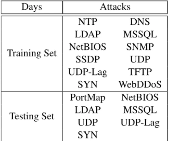
As previously mentioned, this dataset contains both regular traffic and a wide arrange of com-mon DDoS attacks in form of PCAP files. To generate regular traffic, they simulate the abstract behaviour of 25 users based on machine learning algorithms were that trained on real usage of application protocols. The attack traffic was generated on a two-day period, each with a different set of types of DDoS attacks, as displayed on Table5.1.

It also provides Comma-Separated Values (CSV) files with the 80 statistical features extracted from both Linux and Windows firewall log files adding up to 29.40 GB of data. With over 70 million entries, each one is labeled with the attack it was performing according to its source and destination’s IPs and ports, which allows for the establishment of a ground truth.

Days Attacks Training Set NTP DNS LDAP MSSQL NetBIOS SNMP SSDP UDP UDP-Lag TFTP SYN WebDDoS Testing Set PortMap NetBIOS LDAP MSSQL UDP UDP-Lag SYN

Table 5.1: List of DDoS attacks performed on each day.

(48)

32 Methodology and Results

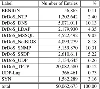
As the classes from the testing set day did not match the classes from training set day, it made little sense to use both sets of data. As such, it was agreed upon that the testing set could be dropped in favour of the other. The proportions of the labeled categories in this dataset can be seen on Table5.2.

Label Number of Entries %

BENIGN 56,863 0.11 DrDoS_NTP 1,202,642 2.40 DrDoS_DNS 5,071,011 10.13 DrDoS_LDAP 2,179,930 4.35 DrDoS_MSSQL 4,522,492 9.03 DrDoS_NetBIOS 4,093,279 8.18 DrDoS_SNMP 5,159,870 10.31 DrDoS_SSDP 2,610,611 5.22 DrDoS_UDP 3,134,645 6.26 DrDoS_TFTP 20,082,580 40.12 UDP-Lag 366,461 0.73 SYN 1,582,289 3.16 total 50,062,673 100.00

Table 5.2: List the different labels and their proportions in the ground truth dataset.

Given this disproportionate ratio between attack and normal traffic, it was decided experiments would be executed with only 1%, 0.1%, 0.01%, and 0.001% of randomly selected attack data, while keeping the normal traffic untouched. This would also allow us to see how these different ratios would affect the performance of all algorithms. Despite only experimenting with binary classification, the system developed can be set to multinomial classification instead of binary.

Nonetheless, it was still considered interesting to perform an experiment with all the data to see if the the algorithms performed similarly well. The complete list with all the attack-benign traffic ration can be consulted on Table5.3.

Attack% Attack-benign ratio Attack-benign entries 100% 0.9987-0.0013 8,395,536-10,700 1% 0.90-0.10 83,795-10,804 0.1% 0.47-0.53 8,350-10,571 0.01% 0.08-0.92 817-10,805

Table 5.3: The attack-benign traffic ration on the final dataset, for each attack percentage of the original dataset.

For all algorithms, it was decided that the split between training and test data would be the traditional 70-30%, respectively, and the metrics used for evaluating each algorithm’s performance were the ones provided by the Science-kit Learn [34] metrics module, namely: Area Under the Receiver Operating Characteristic Curve (AUC), F1 score (F1-s), Precision, and Recall.

Analysis of Intrusion Detection Log Data on a Scalable Environment

F

E

U

P

Analysis of Intrusion Detection Log

Data on a Scalable Environment

Rui Miguel Almeida Oliveira

Abstract

Acknowledgments

Contents

List of Figures

List of Tables

Listings

List of Symbols

Chapter 1

Introduction

1.1

Background and Problem Definition

1.2

Motivation

1.3

Contribution

1.4

Dissertation Structure

Chapter 2

Technological Background

2.1

Firewalls

2.2

Intrusion Detection Systems

2.3

Data Analytics

2.4

Distributed Denial of Service attacks

Chapter 3

State of the Art

3.1

Firewall log analysis and rule inference

3.2

Firewall rule efficiency analysis through log mining

3.3

Malicious traffic detection through firewall log analysis

3.4

Detecting DDoS attacks with Machine Learning

3.5

Summary

Chapter 4

Scalable Intrusion Detection

4.1

IDS log Capturing

4.2

Ground truth collection for training

4.3

Log features used for classification

4.4

Pipeline

4.5

Classification Models

Chapter 5

Methodology and Results

5.1

Dataset description