A platform for assessment of energy recovery technologies by pressure reduction in water distribution networks

Licenciada em Ciências da Engenharia Eletrotécnica e de Computadores

A platform for assessment of energy recovery

technologies by pressure reduction in water

distribution networks

Dissertação para obtenção do Grau de Mestre em

Engenharia Eletrotécnica e de Computadores

Orientador: João Miguel Murta Pina, Professor Auxiliar, FCT

Co-orientadora: Helena Margarida Ramos, Professora Auxiliar, Instituto Superior Técnico

Júri

Presidente: Doutor Rodolfo Alexandre Duarte Oliveira - FCT/UNL Arguente: Doutor Mário Fernando da Silva Ventim Neves - FCT/UNL

Copyright © Ana Filipa Ferreira Sebastião, Faculty of Sciences and Technology, NOVA University of Lisbon.

The Faculdade de Ciências e Tecnologia and the Universidade NOVA de Lisboa have the right, perpetual and without geographical boundaries, to file and publish this dissertation through printed copies reproduced on paper or on digital form, or by any other means known or that may be invented, and to disseminate through scientific repositories and admit its copying and distribution for non-commercial, educational or research purposes, as long as credit is given to the author and editor.

Este documento foi gerado utilizando o processador (pdf)LA_{TEX, com base no template “novathesis” [1] desenvolvido no Dep. Informática da FCT-NOVA [2].}

Quero começar por agradecer ao meu orientador, o Professor João Murta Pina por toda a ajuda e paciência que teve durante a realização deste trabalho. À minha co-orientadora a Professora Maria Helena Ramos do Instituto Superior Técnico e ao seu doutourando Modesto Pérez, bem como a toda a equipa do Laboratório de Hidráulica um muito obrigada.

Quero também agradecer a todos os intervenientes que de uma forma ou de outra permitiram que este protótipo fosse construído: ao DEE; à Nova ID; À Henriques e Henriques; à KSB; à Caprari Portugal; à Janz Contadores de Água; à HidroGrés; à Candeias e Filhos; ao RICS Lab e a todos aqueles que aqui não estando aqui mencionados não são menos importantes.

Agradecer ao DEE todas as condições oferecidas durante a realização do curso e da dissertação. A todos os docentes que me acompanharam ao longo do meu percurso académico e a todos aqueles que de uma forma ou outra contribuiram para a minha formação enquanto enquanto aluna de uma prestigiada escola de engenharia e enquanto pessoa.

Quero agradecer ao meu colega António Rosa (’Toni’) por ter sido o melhor companheiro nesta viagem académica recheada de altos e baixos, um amigo que conto levar para a vida.

À minha amiga Sardinha por tantas e tantas vezes ter sido o meu apoio, a irmã, a cozinheira, a lurdinhas, entre outros, uma vezroomates, para sempreroomates.

Aos meus amigos fora do curso: Bianca, Carol, Gabriel, João, Marie, Raquel V., Raquel C., Rita e Zé por sempre acreditarem em mim e estarem sempre presentes.

A todos aqueles que o curso me trouxe e que hoje são amigos.

Aos meus pais e à minha pequena irmã, obrigada por tudo. E mais qualquer coisa, as palavras serão sempre insuficientes, há coisas que não se explicam, sentem-se. Obrigada por serem os pilares da minha vida. Obrigada.

Aos meus avôzinhos e avózinhas, tios e tias, primos e primas por nunca duvidarem das minhas capacidades e por terem o maior orgulho em mim, seja lá o sítio onde estiverem. Um especial obrigada aos meus tios e prima da Margem Sul por toda a ajuda, uma parte desta caminhada foi deita com o vosso apoio.

Over the last century, a giant leap in technological advancement has taken place. Technological progress is being made every day in a wide range of areas. But there are still problems to solve, such as large-scale energy storage and clean energy production.

The goals set by the European Community are clear: fossil fuels must be replaced by renewable energy sources in order to minimize the effects of global warming as well as to

enable a sustainable development for future generations.

However, due to high volatility of renewable energy sources, such as solar, wind and water, there are still many challenges both at production side and upon control strategies, but these challenges have never been so big. Therefore, the production of energy in small installations is becoming an alternative, as a decentralized source of energy production.

In this study, a small-scale system aiming energy recovery through the reduction of pressure in water distribution networks is proposed. A pump operating as a turbine attached to an electrical generator is used to recover the energy that in normal operating conditions would be lost as heat.

The developed system also has educational and research purposes, allowing the develop-ment of new control techniques as well as of new power converters. In order to evaluate the operation of the proposed system, a prototype was created allowing the injection of the recovered energy in the distribution network.

The proposed methodology contemplates a theoretical design, the prototype construction, the definition of possible tests and validation and verification of the collected information. This system developed in this dissertation allows demonstrating the proposed concept, recovering energy without compromising the supply of final consumers.

Ao longo do último século, deu-se um passo gigante no avanço tecnológico. Existem desenvolvimentos diários numa vasta gama de tecnologias. No entanto, existem diversos problemas ainda por resolver, como o armazenamento de energia em larga escala ou a produção de energia cada vez mais limpa.

As metas impostas pela Comunidade Europeia são claras, referindo que a dependência de combustíveis fósseis tem de ser substituída por fontes de energia renováveis, de modo a minimizar os efeitos do aquecimento global, bem como a permitir um desenvolvimento sustentável para as gerações vindouras.

Neste estudo, propõe-se criar um sistema de pequena escala que permita recuperar energia através da redução de pressão em redes de distribuição de água. Uma bomba a funcionar como turbina, solidária com um gerador eléctrico, é utilizada para recuperar energia que, em condições normais de funcionamento, seria perdida sob a forma de calor. O sistema tem também um carácter educativo que permitirá o desenvolvimento de novas técnicas de controlo bem como de novos conversores de potência.

De modo a avaliar a operação do sistema, foi criada uma instalação que permitirá a injecção da energia produzida na rede. A metodologia utilizada para concretizar o objectivo inicialmente proposto contempla o dimensionamento teórico, a implementação da instalação, a definição de possíveis ensaios e a validação e verificação da informação recolhida.

O sistema desenvolvido na presente dissertação permite demonstrar o conceito proposto, a recuperação de energia sem comprometimento do abastecimento do consumidor final.

List of Figures xvii

List of Tables xxi

Acronyms xxiii

1 Introduction 1

1.1 Context . . . 1

1.2 Objectives . . . 2

1.3 Dissertation Structure . . . 2

1.4 Acknowledgements . . . 3

2 Literature Review 5 2.1 Basic Hydraulic Concepts . . . 5

2.1.1 Principles of Fluid Dynamics . . . 8

2.1.2 Fundamental Principles of Hydrokinetics and Hydrodynamics . . 9

2.2 Water Distribution Networks . . . 11

2.2.1 General Overview . . . 11

2.2.2 Piping . . . 12

2.2.3 Connection Points . . . 12

2.2.4 Valves . . . 14

2.2.5 Portuguese Regulation . . . 14

2.3 Turbomachinery . . . 17

2.3.1 Turbines . . . 18

2.3.2 Pumps Classification . . . 26

2.4 Pump as a Turbine . . . 28

2.5 Electrical Drive . . . 29

3 Experimental Setup 33 3.1 Design . . . 33

3.1.1 System Design Parameters . . . 34

3.1.2 Pipe Design . . . 35

3.1.4 Reservoirs . . . 41

3.1.5 Measurement Devices . . . 43

3.2 Computational Design: EPANET . . . 45

4 Material Selection and Implementation 47 4.1 Material Selection . . . 47

4.1.1 Pipes . . . 47

4.1.2 Fittings . . . 48

4.1.3 Pump and PAT . . . 50

4.1.4 Measurement Instruments . . . 53

4.2 Implementation . . . 57

5 Experimental Results 75

6 Conclusions 83

Bibliography 85

I Local Losses Coeffi_{cients 91}

II Unit Conversion Tables 97

III EPANET 99

IV PAT Data Sheet 101

V Pump Data Sheet 105

VI Induction Machine Data Sheet 107

2.1 Illustration of static pressure measurement . . . 6

2.2 Eff_{ect of pressure increase with velocity decrease . . . . 7}

2.3 Fluid Flow Regime: Laminar and Turbulent . . . 10

2.4 Distribution system in Hodaidah, adapted from [7] . . . 12

2.5 Steel pipe . . . 13

2.6 PEAD pipe . . . 13

2.7 Welding of steel pipes, adapted from [7] . . . 13

2.8 DI Fittings (Manufacturer: Saint-Gobain) . . . 14

2.9 Pressure Reduction Valve from Hawle company . . . 14

2.10 Ball Valve from Pinto e Cruz company . . . 15

2.11 Pumps and Turbines . . . 18

2.12 Hydraulic Machines . . . 19

2.13 Turbine scheme . . . 19

2.14 Impulse Turbine . . . 20

2.15 Pelton Turbine . . . 21

2.16 Regulating of speed . . . 22

2.17 Bucket: pelton vs turgo, adapted from [15] . . . 22

2.18 Turgo Turbine: Angle of strike, adapted from [16] . . . 23

2.19 Crossflow Turbine, adapted from [16] . . . 24

2.20 Francis turbine: runner . . . 25

2.21 Section of an Axial flow (propeller) turbine, adapted from [9] . . . 25

2.22 Pump . . . 26

2.23 Pumps Classification, adapted from [17] . . . 27

2.24 Main Components of hydropower generation, adapted from [49] . . . 29

2.25 Fixed-Speed Turbine, with an induction generator, adapted from [51] . . . . 30

2.26 Variable-Speed Turbine, with a doubly-fed induction generator, adapted from [49] . . . 30

2.27 Variable-Speed Turbine, with a synchronous generator, adapted from [49] . . 31

3.1 Design Experimental Unit . . . 34

3.2 Calculation of inlet diameter . . . 36

3.4 Pump as a Turbine (PAT) Curve . . . 40

3.5 Pump:Characteristic Curve C . . . 40

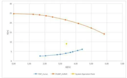
3.6 Pump Curve, PAT and system operation point . . . 41

3.7 Reservoir Example . . . 41

3.8 System connection . . . 42

3.9 Possible operation scenarios . . . 42

3.10 Hydropneumatic reservoir . . . 43

3.11 Manometers example: with and without glycerine . . . 43

3.12 Flow meter, from Resopre-Janz Company . . . 44

3.13 Pull-Down Resistor . . . 44

3.14 EPANET:Simulation of system pressure (P<25m) . . . 45

3.15 EPANET:Simulation of system flow (Q<25l/s) . . . 45

4.1 Circulation Pump . . . 50

4.2 Pump as a turbine (PAT) . . . 51

4.3 Initial reservoir of 250 L capacity . . . 52

4.4 Hydropneumatic reservoir and components . . . 52

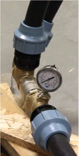
4.5 Manometer . . . 53

4.6 Flow meter . . . 54

4.7 Energy Analyser . . . 55

4.8 Autotransformer’s . . . 55

4.9 Assembly Draft . . . 58

4.10 Brass deposit cannon . . . 59

4.11 Reservoir exit:1. Discharge reservoir, 2. Brass deposit cannon, 3. Ball valve, 4. Male adaptor, 5. Pipe . . . 59

4.12 Fitting constitution - 1. Body, 2. O-ring, 3. Blocking bush, 4. Clinching ring, 5. Cap nut . . . 59

4.13 Initial pump:Inlet, outlet and pipe material . . . 60

4.14 Hdropneumatic reservoir exit:1. Hydropneumatic reservoir, 2. Flange DN65, 3. M16 hexagon head screw, 4. Reducing nut, 5. Double male bushing, 6. Ball valve, 7. Double male bushing, 8. Female union, 9. Female adaptor . . . 60

4.15 Flow Meter Installation . . . 61

4.16 Manometer installation. . . 61

4.17 PAT: 1. Female adaptor, 2. Double male reducing bushing, 3. union, 4. Male adaptor . . . 62

4.18 PAT: 1. Female adaptor, 2. Reducing tee, 3. Reducing nut, 4. Ball valve, 5. Tee, 6. Elbow, 7. Manometer, 8. Reducing nut . . . 62

4.19 Auxiliary Switchboard with interrupters and protection . . . 64

4.20 Pump Autotransformer . . . 65

4.21 . . . 66

4.23 Pump: Terminal Box and Coils Connection . . . 67

4.24 Pump as a Turbine Autotransformer . . . 67

4.25 Pump as a Turbine: Terminal box and coils connection . . . 68

4.26 Pump as a turbine: 1. Terminal box, 2. From autotransformer, 3. To power Analyser . . . 68

4.27 Arduino Uno and Inductive Sensor: Connection scheme . . . 69

4.28 Experimental unit (final Setup) . . . 70

4.29 Test rig kick-off . . . 71

4.30 Midlle state of the development . . . 72

4.31 Conclusion . . . 73

5.1 PAT: Direct on-grid connection . . . 76

5.2 Steinmetz scheme per phase . . . 76

5.3 Simplified scheme with power flow . . . 76

5.4 Test ID #1: Voltage and active power profile . . . 78

5.5 Test ID #2: Voltage and active power profile . . . 79

5.6 Test ID #3: Voltage and Active Power profile . . . 80

5.7 Induction machine as a motor (point 2 from test ID #2) . . . 81

3.1 Surface roughness (k) for pipes . . . 38

3.2 Pipe Bend: Local losses coefficient_⇣. . . 38

3.3 Tee: Local losses coefficient_⇣ . . . 38

3.4 Nominal diameters millimetres vs inches . . . 39

3.5 Total Head loss . . . 39

4.1 Pipe materials: Advantages and disadvantages . . . 48

4.2 Fitting Types . . . 49

4.3 Circulation Pump: Characteristics . . . 50

4.4 PAT: Hydraulic characteristics . . . 51

4.5 PAT: Electric Characteristics . . . 51

4.6 Inductive Sensor . . . 55

4.7 Total Head loss . . . 70

5.1 Experimental Results for a PAT . . . 77

5.2 Test ID #1: Resume . . . 78

5.3 Test ID #2: Resume . . . 79

EN European Norm.

PAT Pump as a Turbine.

PDP Positive Displacement Pump.

PEAD High Density Polyethylene.

PRV Pressure Reduction Valves.

PVC Polyvinyl Chloride.

Chapter

1

I n t r o d u c t i o n

The fast growing of the worldwide population is causing not only an increase in energy demand but also a concern among the specialists about environmental issues, leading to new studies and innovative solutions applied to the energy sector. One of the main boosters has been the identification of new technologies, capable of satisfying the needs of final consumers while being an alternative to energy production from fossil fuels.

The available resources to energy production, like the sun and the wind, are in many cases unpredictable solutions, needing in all cases backup solutions.

Renewable energy sources already fill consumers needs but due to their unpredictability, alternative renewable energy solutions must be developed. However, there are in many cases systems that can be optimized and which ultimately allow the use of energy which would be wasted in normal conditions.

A system to recover energy in a water distribution network is presented.

1.1 Context

Over the years, the planet demands for new strategies in order to prevent global warming and according to the Directive 2009/28/EC of the European Parliament EU, members must guarantee that 20 % of the consumption in UE is derived from to renewable energy sources, and also a decrease of 20% in CO2 emissions when compared to 1990.

The energy consumption in all the process that involves water (distribution, transport, recycling, irrigation) is an area of study that is quite underdeveloped by the fact that there are different variables that can influence the energy patterns of usage, according

to a survey held by an ACEEE - American Council for energy. The same study also suggests that there are additional oportunities for energy efficiency as well as for water

According to recent studies, water supply systems worldwide can have energy losses of, on average, 40 per cent from the total water consumption. Such topic has concerned not only the environment experts but also managers of water supply systems. This concern is focused on the quest for economic and environmental self-sustainability of water distribution networks, which involves an high energy consumption and pressure control.

Moreover, several authors supported the use of pumps as turbines operating in water distribution networks, as a valuable solution not only for populations supply and irrigation, but also for energy production in a micro-scale, in a context of renewable energy production, with the advantage of a low cost installation and also because it is environmentally friendly. Economically, the choice of using a pump is only applicable if there is an excess of energy in the network, which in normal conditions would be lost, or if the output power generated by a turbine is too low (low flow).

According to [2] the use of pumps as turbines can be an alternative to common turbines not only because they are cheaper but also because they have a wide range of models available.

1.2 Objectives

Despite some studies in this field, the objective of this master thesis was to prove that a pump working as a turbine, inserted in a water distribution network, can produce energy and explore new techniques and control strategies, giving also the possibility to use a pump as a turbine in the network as a replacement of pressure reduction valves.

In order to demonstrate this concept a prototype was set up in a laboratory context at FCT NOVA whose main objective was to prove energy recovery but also to be used with an educational and research purpose.

This work includes a theoretical design, assembly and test of the experimental setup.

1.3 Dissertation Structure

This master thesis is divided in six chapters:

• Chapter One - Introduction to the developed work and the objectives to be achieved.

• Chapter Two - Literature review with the presentation of hydraulic concepts, relevant legislation and network electric connections.

• Chapter Three - Presentation of the system design.

• Chapter Four- Material selection and implementation, explanation of the methodology used for both material selection and system implementation .

• Chapter Six - Main conclusions about the developed work and possible future work.

1.4 Acknowledgements

Chapter

2

L i t e r a t u r e R e v i e w

Water is the driving force of all nature.

Leonardo da Vinci

This chapter provides an overall view of energy production by performing a pressure reduction in Water Distribution Networks as well as discuss the actual technologies and proposed solutions for this problem. It gives a brief explanation of the fundamental principles behind it.

A contextualisation about Portuguese regulation is also made so that experimental setup and test conditions are brought together as close to reality as possible.

2.1 Basic Hydraulic Concepts

In this section a description of principles and concepts that support the initial idea of this work.

• Flow

Flow is defined as the amount of a certain fluid that passes through a surface (pump or turbine) within a period of time. Two parameters of flow can be considered: volume flow (Q) and mass flow (Qm). Volume flow, which can be read from a pump/turbine

curve, is the quantity of volume that a pump/turbine can move per unit of time. This parameter is measured inm3/hand is independent from the liquid density (⇢). On the other hand, mass flow (Qm) is the mass of fluid moving per unit of time. This parameter

Qm=⇢Q (2.1)

• Pressure

Pressure is defined as force per unit of area. The total pressureptotal of a fluid is the

sum of its staticpstatic and dynamic pressurepdynamic.

Static pressurecan be measured with a pressure gauge placed perpendicular to the fluid flow or in an non moving fluid, see figure 2.1.

Figure 2.1: Illustration of static pressure measurement

Dynamic pressureis dependent on fluid velocity (v) and density (⇢), and cannot be measured using a pressure gauge. Instead, it is calculated using the equation 2.2.

pdynamic=

1

2⇢v2 (2.2)

Dynamic pressure is specially important because it can be converted into static pressure when the velocity of fluid changes. When the pipe diameter increases fromD1toD2, the liquid velocity will decrease from v1 to v2 (figure 2.2). If the effect of friction loss is neglected, the sum of static and dynamic pressures is constant through the horizontal pipe, see equation 2.3.

p₁+1 2⇢v1

2_=p

2+1₂⇢v22 (2.3)

As shown in figure 2.2, when the diameter is increased, the static head, measured in pressure gaugep2, will also increase.

In most pressurised systems the effect of dynamic pressure is negligible when calculating

the head of a pump/turbine.

Pressure can be measured in different units depending on application, see Appendix

Figure 2.2: Effect of pressure increase with velocity decrease

is to know the exact point of reference for pressure measurement. So, it is essential to know the absolute and the gauge pressure:

• Absolute pressure is the reference value (absolute zero for pressure 0 atm). This parameter is specially important in cavitation calculation.

• Gauge Pressureis the pressure above normal atmospheric pressure (1 atm). Usually the measurement devices calculate the difference between the system pressure

(gauge pressure) and the atmospheric pressure.

Headis an expression that allows determining how high the pump can lift a liquid. It is measured in meters and is independent from the liquid density. Equation 2.4 shows the relation between pressure and head. Usually the values defined by manufactures are expressed inbarwhich is equal to 105Pa.

H= p

⇢g (2.4)

Where,

His the head [m]

pis the pressure [Pa=N /m2]

⇢is the liquid density [kg/m3] gis the acceleration of gravity [m/s2]

Energy conversion

Hydropower generation has as a principle the conversion of hydraulic potential energy of a flow into electric energy, which corresponds to a diff_{erential net head, usually}

denominated as"H".

The principle of energy conservation, the energy balance of a steady flow from an arbitrary point A to an arbitrary point B will obey Bernoulli equation (2.5):

ZA+

pA ⇢g +

↵AVA2

2g =ZB+ pB ⇢g+

↵BVB2

2g +∆HAB (2.5)

whereZ is theelevation head(m) at the point of interest (above a reference plane); pA and pB (Pa) is the pressure at the center of gravity of the flow cross sections; V

(m/s) is the average flow velocity;⇢(kg/m3) is the water density,g(m/s2) is the gravity acceleration and↵ represents the numerical coefficient accounting for the non-uniform

velocity distribution; equation 2.5 expresses the difference between total heads at A (_HA)

and B (HB) is equal to the headloss∆HABbetween the two flow cross sections, where the

head is the total flow energy by weight of the flowing water, [3].

2.1.1 Principles of Fluid Dynamics

In this section the fluid properties will be described. A fluid can be either a liquid or a gas, and its defined by the deformation under an applied shear stress (equation 2.6).

⌧= F

A (2.6)

where,⌧ is the shear stress expressed in Pa;F the applied force, expressed in N or

kg·m/s;Athe cross sectional area of a material parallel to applied force, expressed in m2.

• Water properties: Density, Fluid Mass and Weight

Density⇢is used to define and characterize the mass of a fluid system. In SI Units the density is expressed in kg/m3_{. Variations in pressure and temperature will have a} small effect in_⇢, most of the times the value is nearly constant; the density of water is

about 1000 kg/m3at 20 C.

Anther important relation is specific volume,⌫= 1_⇢ and is the volume per unit mass (inversely proportional to density).

Specific weight is the weight of a fluid per unit volume, and this value is related to the density =⇢g. This value, expressed in N/m3, is used to characterize the weight of

the system. Under conditions of standard gravity (g= 9.807 m/s2), water at 20 C has a specific weight of 9790 N/m3_.

• Viscosity

Viscosity (µ) is the quantitative measure of a fluid’s resistance to flow. The previous

properties of fluid (⇢e ) are not enough to characterize how fluids behave. Two fluids (water and oil) can have approximately the same value of density.

Viscosity is defined as:

⌧=µ@u

where viscosityµis expressed in kg/m·s; differential equation @_@u_y defines the slop of

each line, depending on material; u

y is the rate of shear deformation.

Equation 2.7 can be used where velocity does not vary linearly withy, such as, fluids

moving through a pipe.

• Compressibility

Compressibility is a fluid property, directly related with the volume change of a fluid. A fluid is defined as a substance that deforms continuously when acted under the influence of a force. The force is created whenever a tangential force acts on a surface. Generally, fluids can be compressible (e.g. almost every gas) or incompressible (e.g. water). In the case of compressible fluids their volume is dependent on pressure and temperature. Liquids can be considered as incompressible for almost every engineering application (except in hydraulic shock calculation) as their volume is independent from pressure. For example, at atmospheric pressure and 20 C it would require a pressure of 215 bar to compress a unit volume of water only 1%. The pressure to cause an exchange in volume is too large.

• Vapor Pressure

Vapor pressure is the pressure at which a liquid boils. Water vapor pressure at 20 C is 2330 N/m2and at 100 C is equal to the normal atmospheric pressure.

When the pressure of a liquid drops to the respective vapor pressure the liquid starts to boil. If the drop in liquid pressure is due to fluid flow, vapor bubbles can be formed. This process is called cavitation.

2.1.2 Fundamental Principles of Hydrokinetics and Hydrodynamics

In this section fluids main characterization based on flow type will be explained.

• Basic Concepts

Water flow/Discharge is defined as the volume that crosses a section per unit of time.

Q=R_sV ds=V·A

• Fluid Flow Regime

Fluid flow can be categorized according to different criteria such as its variation

through time, space and flow pattern.

Analysing a fluid flow through time, it is possible to classify it as steady or unsteady. If there are variations in velocity, pressure, density and discharge, for a certain period of time, the fluid is classified as unsteady. Steady flow is rare in a practical scenario.

When the flow of a fluid is moving with a moderate speed, the fluid has fluid layers moving past each other. Such type of flow is designated as laminar flow. For a laminar flow in a pipe, only one component of velocity is defined (equation 2.8). This is a type of flow characterized by smoothness and regular trajectories of fluid particles.

V =u_e#»

x (2.8)

whereV represents the the punctual velocity, expressed in m/s and_e#»

xxrepresentsx

component of the velocity curve as a function of time at a point A in the flow.

On the other hand, when the flow speed of one calm layer increases, these smoothly moving layers start moving randomly and will increase the flow velocity, the fluid particles become completely random and no such laminar layers exists any more. In this kind of turbulent flow, the main component of velocity along the pipe is unsteady (random) and accomplished by random components normal to the pipe axis, see equation 2.9.

V =ueˆx+veˆy+weˆz (2.9)

where V is the punctual velocity, expressed in m/s; _e#»

x, e#»x and e#»z are the normal

components along the pipe axis.

It is possible to observe those types of fluid flow regime in domestic places, after the opening of a tap, before the water reaches the sink; laminar flow is presented, after the water reaches the sink, the flow is characterized as turbulent, figure 2.3 illustrates the effect of both fluids passing through a fluid body.

Figure 2.3: Fluid Flow Regime: Laminar and Turbulent

Shear stress in turbulent flow is larger than those in laminar flow [4].

The Reynolds number, defined in equation 2.10, is the ratio of inertia to viscous effects

in the flow. This number is used as a criteria to distinguish between laminar and turbulent flow and will increase with the flow velocity of the initial forces. The flow in a round pipe is laminar if the Reynolds number is less than approximately 2100 and when the value is greater than 4000 the flow is turbulent. Flow can change between laminar and turbulent conditions in a randomly way. This state is considered the transitional flow.

Re=⇢V D

µ (2.10)

whereReis the Reynolds Number, expressed in (kg·m/s2)/N but, since 1 N = kg·m/s2

this is a dimensionless parameter;⇢is the fluid density, expressed in kg/m3_{;V the mean} fluid velocity, expressed in m/s;Dthe pipe diameter, expressed in m;µthe fluid viscosity, expressed in N·s/m2.

Reynolds number is specially important in losses calculation; a detailed explanation is found in chapter 3.1.2.

2.2 Water Distribution Networks

In this section what is a water distribution network and its main elements as well as how Portuguese Regulation defines such type of network is explained.

2.2.1 General Overview

Water distribution systems provide water for human consumption, piped water is also used for washing, sanitation, irrigation and fire-fighting. However, before the water reaches the final consumer many processes are behind it: capture, treatment, elevation, transport, storage and distribution, [5].

The water supply system can be divided in three main stages [6]:

• Raw water extraction and transport;

• Water treatment and storage;

• Clean water transport and distribution.

In both transportation and distribution, water is conveyed through a network of pipes, stored in the middle points and pumped if necessary, to guarantee the desired pressure and demand, that can vary through different parts of it. This is a factor that has a huge

2.2.2 Piping

Pipes are one of the most important components in water networks (distribution and transport) because they allow to carry the water from a certain point A to B and reach the final consumer.

Pipes can be made of different materials, may have different diameters, service connections

or valves. Pipe specifications will depend on the final purpose.

Depending on the site location of the water sources, the pipe diameters will change. Figure 2.4 represents a water distribution network with different pipe diameters that

supplies around 350.000 consumers.

The water, in this case, is pumped from the reservoir via a main trunk (D= 600 mm)

for the secondary network with pipe diametersD=300-500 mm and then distributed by

the pipesD= 100 andD= 200 mm. Pipes diameter will decrease as the consumption point approaches.

Figure 2.4: Distribution system in Hodaidah, adapted from [7]

Pipes material must be carefully chosen during the design phase, material choices as steel pipes can lead to rust formation as a result of aging process. So, there are a lot of possibilities: CI (cast iron), steel, PVC (Polyvinyl chloride) and GRP (Glass Reinforced Pipes). According to [8] when comparing CI pipes to PVC Pipes, CI pipes required higher standards in water treatment when compared to other pipe materials.

A detailed example of two different pipe materials are presented. A steel pipe (figure

2.5) and a PEAD (high density polyethylene) pipe (figure 2.6).

2.2.3 Connection Points

There are several types of joints that can be used to connect the diff_{erent pipes in a}

network: rigid, semi-rigid and flexible.

Figure 2.5: Steel pipe

Figure 2.6: PEAD pipe

Sometimes the solution to connect two pipes implies welding. This is the cheapest join junction for steel pipes of larger diameters (2.7), although these joints do not allow any pipe route deflection and change in direction.

Figure 2.7: Welding of steel pipes, adapted from [7]

Another example of connection points are fittings, see figure 2.8, mostly used when there is a change in pipe diameter and/or material, pipeline direction or when it is necessary to install valves or measurement devices.

Figure 2.8: DI Fittings (Manufacturer: Saint-Gobain)

2.2.4 Valves

Another important element in Water Distribution Network (WDN) are the valves. There is a widely range of models available in the market, and each application can have a different type of valve.

Valves have three main tasks, [6]:

• Flow and/or pressure regulation (flow control valves, pressure reducing or pressure sustaining valves, etc.);

• Exclusion of parts of the network in order to execute maintenance or emergency operations (section valves);

• Protection of the reservoirs and pumps (e.g. float valves, non-return valves).

For the purpose of this study the most important valves are the ball valve (figure 2.10) and the pressure reduction valve (figure 2.9).

Figure 2.9: Pressure Reduction Valve from Hawle company

2.2.5 Portuguese Regulation

Figure 2.10: Ball Valve from Pinto e Cruz company

• Legislation

In Portugal the legislation for water distribution networks follows the Regulatory Decree no. 23/95 of 23th of August, DR 23/95, with the definition of the rules for public and building systems of drinking water distribution and drainage of waste water. This Decree is based on an adaptation of an European standard European Norm (EN) 806 which specifies installations inside buildings conveying water for human consumption.

However, under the article no. 2 of DR 23/95 each city must adapt the current legislation and create specific norms. Water supply and distribution is regulated by three type of entities: city councils, municipal companies and private companies. Those are called service providers, and diff_{erent management models are possible.}

• Hydraulic Design (according to DR 23/95)

The design of a water distribution network must be done according to the minimum consume demand. The design must consider the number of inhabitants as well as their needs. For example, assuming a population with more than 50,000 inhabitants the minimum consume is 175 L/inhabitant/day. There are also some consume references for special buildings such as schools, hotels, restaurants, hospitals and emergency networks.

According to DR 23/95, in building branches minimum and maximum pressures of respectively 100 kPa (1 bar) and 600 kPa (6 bar) are established. Concerning flow the numbers are between 80-175 L/inhabitant/day for an inhabitants range from 1,000 to 50,000.

The maximum, statics and service, pressure measured at the sea level must be under 600 kPa (6 bar). During the day, the maximum variation is 300 kPa (3 bar), in each node of the system.

For the hydraulic design, flow velocity, during peak hours, must be bellow 0.5-20 m/s. This value is given by equation 2.11.

V = 0.127D0.4 (2.11)

whereV is the limit fluid velocity, expressed in m/s;Dis the intern diameter of the

It is also established that the minimum nominal diameter for distribution is 60 mm (for locations with less than 20,000 inhabitants).

• Type of material

Regarding the type of material of the pipes, the regulation defines that it can be:

• Asbestos cement;

• Cast iron;

• Copper;

• Stainless steel;

• Galvanized iron or steel;

• Polyvinyl Chloride (PVC);

• High Density Polyethylene (PEAD);

• Other types of material that gather the proper conditions.

• Branch connection

Connection branches with building systems must be done with good conditions of pressure and flow in order to guarantee a good quality of the service.

The minimum flow is specified in the design of building systems, and the fluid flow velocity must be between 0.5 m/s and 2 m/s, according to the available pressure in the network.

After the distribution network the minimum diameter of branch pipes is 20 mm. Fittings and accessories for connecting elements must assure no leaks and an easy manoeuvre in case of a major trunk in the network (fault case).

Each and every network needs to be equipped to respond if any fault occurs. The network must have isolation valves placed in strategic points, allowing an easy operation with no interruption of the supply. This type of valves must be placed in:

1. Branch connections;

2. Before and after network elements, to provide a quick response, in case there is a need to replace or restore one;

3. Along the distribution line (no more than 1,000 m spacing);

The installation of pressure reduction stations is mandatory in order to decrease the pressure downstream. These stations are equipped with Pressure Reduction Valves (PRV) installed in accessible places. Downstream must be equipped with a sand filter and upstream with a manometer or with a device that allows an easy pressure management. PRV upstream and downstream must have isolation valves, as well as a bypass system in order to guarantee system efficiency.

Water distribution networks must have active devices to measure the amount of water flowing. Flow meters must be installed in protected and accessible places to allow a correct measurement. Furthermore, flow meters must be placed in building systems of all end consumers, output reservoirs, pumping stations and strategic places to allow system efficiency measurement. There are different types of parameters to consider when

selecting a flow meter, for example, the range of flows to be measured, required precision, maximum head loss, service pressure, diameter and pipeline position.

2.3 Turbomachinery

The prefix turbo derives from the latin’turbo’meaning "spin"or "whirl".

Turbomachines are devices that transfer energy either to, or from, a moving flowing fluid by the dynamic action of one or more moving blade rows, converting hydraulical energy into mechanical energy and vice-versa.

Turbomachines are divided in two big groups: those that supply energy to the fluid, calledpumps, and those that extract energy from the fluid, calledturbines[3].

A rotor or an impeller can do positive or negative work, depending on the required effect in the machine. These momentum changes are linked with pressure changes that

occur due to fluid movement, see figure 2.11, [9]. Rotor and impeller are connected to a rotating shaft, hence the name tubomachinery.

Based on the flowing fluid, turbomachines can be classified as:

1. Hydraulic machines (incompressible fluids): pumps, hydraulic turbines, fans, marine propellers;

2. Thermal machines (compressible fluids): gas turbines, vapor turbines, compressors, airplane propellers, wind turbines.

In hydraulic machines, turbines and pumps have different characteristics and applications,

and they can be classified in different ways, according to figure 2.12.

As the fluid particle moves, both gravity and pressure forces do work on the particle. Recall that the work done by a force is equal to the product of the distance the particle travels times the component of force in the travel direction.

Figure 2.11: Pumps and Turbines

2.3.1 Turbines

Hydraulic turbines are specially designed to convert a certain hydraulic energy (potential and kinetic energy available in water falls) into mechanical energy of rotation that generates electrical energy, see figure 2.13.

Turbines can be diff_{erentiated according to:}

1. Operating head:

High head: above 300 m e.g. Pelton wheel;

Medium head: 30-300 m e.g. Francis Turbine;

Low head: 3-30 m e.g Kaplan Turbine.

2. Direction of the internal flow, [10]:

Tangential Flow: Flow tangent to the rotor;

Axial Flow: Flow without significant radial component in the rotor (e.g. Kaplan

Turbine);

Radial Flow: Flow with significant radial component at the rotor outlet or inlet (e.g.

Figure 2.12: Hydraulic Machines

Mixed Flow(e.g. Pelton wheel)

3. How potential energy is converted into mechanical energy [11]

Impulse turbine(e.g. Pelton)

Reaction turbine(e.g. Francis)

Considering the purpose of this work, only the last classification will be considered.

2.3.1.1 Impulse Turbines

An impulse turbine is characterized by the pumping of the water at a high pressure to a nozzle where it expands to atmospheric pressure. The emerging jet impacts on the blades (or buckets) of the turbine, which produces the required torque and power output, [9], see figure 2.14. In this kind of turbines the flow energy is converted into kinetic energy before transformation in the rotor, making it more suitable for applications that require an high head and low power.

An impulse turbine needs a chase only to control the splashing and to protect against accidents. Usually this kind of turbines are cheaper than reaction turbines because no special pressure chase is needed.

Figure 2.14: Impulse Turbine

Pelton, turgo and cross-flow turbines will be presented in sequel.

• Pelton Turbine

Pelton turbine (free-jet) is the most widely used model of this type. Many variations of impulse turbines existed prior to this one but they were less efficient than Pelton’s design,

2.15 (2) ) and one or more nozzles (maximum 6) (figure 2.15 (3) ) to which the water is supplied from the pipeline (figure 2.15 (4) ).

The runner/wheel consists of a disk with a series of blades (usually called buckets (figure 2.15 (5) )) with the shape of a double spoon, around the periphery. Each bucket has two curvilinear surfaces separated by a spear. The runner and the nozzle are assembled above sea level, for that reason the runner rotates in the air (does not work submerged), figure 2.15. One or more nozzles are mounted in a way that each nozzle directs its jet along the tangent to the circle through the centers of the buckets.

As the jet (figure 2.15 (6) ) hits a bucket, the spear splits the oncoming jet into two equal streams so that each flow goes from on side to the other of the curvilinear surface in a direction nearly opposite that of the incoming jet.

The jet of water coming from the nozzle hits the buckets of the runner which allows the transformation of the kinetic energy of the water into rotational mechanical energy. The nozzle has a movable needle inside which allows the control of the discharge, as shown in figure 2.16b.

The nozzle has also a deflector (figure 2.16) that operates as a device control in case a load rejection occurs, making an alteration of the jet direction enabling its slow closure, which allows to control overpressure in the penstock and overspeed of the runner [12].

The quality of a Pelton Turbine is regulated by the change rate of the water flow throught it, this is ensured by the needle. When the needle covers the totality of the nozzle the flow rate is equal to zero [13].

Figure 2.15: Pelton Turbine

• Turgo Turbine

Turgo turbine was developed by Gilkes Energy Company in 1919 and is a variation of Pelton turbine free jet impulse. It is designed for medium head applications. It is less efficient than a Pelton but it has the capacity to generate the same power, and has a runner

that can deal with high discharge variations [14].

The differences between Pelton and Turgo turbines are the design of the buckets and

a Needle

b Deflector

Figure 2.16: Regulating of speed

centre of the bucket at a right angle and then split into two (figure 2.17a). Unlike the Pelton, in Turgo turbines, the jet is designed to enter the runner in a different angle

(typically 20·C figure 2.18), pass through the wheel, and discharge from the other side

(figure 2.17). Also, the discharged fluid and the incoming jet do not limit the flow rate. Due to these differences, it is possible to have a smaller diameter runner than a Pelton

and achive the same power [15].

a Bucket of a pelton Turbine b Bucket of a turgo Turbine

Figure 2.17: Bucket: pelton vs turgo, adapted from [15]

Figure 2.18: Turgo Turbine: Angle of strike, adapted from [16]

flow with the same diameter as a Pelton, reducing the generator costs which decrease the installation costs. Both turbines can have a horizontal or vertical orientation.

• Cross-Flow Turbine

The cross-flow turbine, also designated by Ossberger, Banki or Mitchell, is used for a wide range of flow and heads between 5 and 200 meters. This turbine has its runner shaft parallel to the ground in all cases, it comprises a drum-shaped runner with two parallel disks connected together near their border by a series of curved blades. In operation, a rectangular jet directs the flow to the full length of the runner. The water strikes the blades and transmits most of its kinetic energy. It then passes through the runner and strikes the blades on the exit, transferring a small amount of energy before leaving the turbine.

Compared to other turbines, cross-flow has a low effi_{ciency that can be improved by}

the inducement of a partial vacuum inside the chasing; such vacuum improvement is expensive since it requires an air seal around the runner shaft as it passes through the chasing. This can be achieved by the placement of a draft tube bellow the runner which remains full of tail water at all times. Any decrease in the water level induces an higher vacuum which is limited by the use of an air bleed valve in the chasing, figure 2.19.

The water passes through a guide-vane located upstream of the runner and has a double action on the blades of the runner.

This simple design makes this turbine cheap and easy to repair in case of runner brakes due to the important mechanical stresses, [9].

It is an alternative when there is enough water, defined power needs and low investment possibilities, such as for rural electrification programs.

2.3.1.2 Reaction Turbines

Figure 2.19: Crossflow Turbine, adapted from [16]

the flow; a draft tube is at the exit of the turbine in order to transform velocity head to static head due to its increasing area. The pressure of the water gradually decreases as it flows through the runner. This type of turbines are so called reaction turbines because of this pressure change [9].

A reaction turbine, apart from the runner, is composed of runner vanes that are curved and surrounded by a guide wheel. They also have a closed chamber (spiral case), where the flow takes place in transforming part of pressure energy into rotational mechanical energy of the runner. A movable guide vane (or wicket gate) guides the flow around the runner, making the regulation of the turbine discharge to the draft tube. The draft tube allows to minimize losses [11].

• Francis Turbine

Francis turbines usually have a vertical axis (small machines can have an horizontal axis). This turbine is of radial or mixed flow with adjustable wicket gate. It is used for low/medium heads and high flow rates.

The water enters through a spiral casing called a volute or scroll that surrounds the runner. The area of cross-section of the volute decreases along the flow path in such a way that the the flow velocity remains constant. After the volute the water enters in a ring of stationary guide vanes that direct the flow in a certain angle according to the demand of power, [9].

While flowing through the runner (figure 2.20), the angular momentum of the water will decrease while work is supplied to the turbine shaft. The flow leaves the runner axially into the draft tube and finally the flow enters the tailrace.

The exit of the draft tube must be submerged bellow the level of the water in the tailrace to guarantee that turbine remains full of water. The draft tube also has the function of diffuser.

Figure 2.20: Francis turbine: runner

Propeller and Kaplan turbines are axial flow reaction type and are specially designed for low heads, these turbines generate power from much lower heads than Francis Turbines. Kaplan turbines can be defined as a more sophisticated version of the propeller turbine [16].

The basic version of propeller turbine consists of a propeller, similar to ship’s propeller, fitted inside a continuation of the penstock tube. Three to six blades are used; in case of very low head units, only three are necessary. This turbine is an option when both flow and head remain constant.

In this kind of turbines the water flow is done by the use of wicket gates just upstream the propeller, figure 2.21.

Figure 2.21: Section of an Axial flow (propeller) turbine, adapted from [9]

On the other hand, Kaplan turbines have adjustable runner blades that can have adjustable guide vanes or not, being classified as double regulated or single regulated, respectively. This feature allows for a better adaptation to different flow values and an

Kaplan turbines differ from propeller turbines by having pitch runner blades, where

wicket gates are carefully designed to induce tangential velocity or ’whirl’ in the water. Both types of turbines can be arranged in an open flume (micro generation) or with a spiral case of concrete or cast iron, similarly to Francis turbines.

2.3.1.3 Pumps

Generally, a pump is a machine that adds energy to anything flowing through it. The spontaneous tendency of anything is to flow from high potential to low potential and this natural tendency is harnessed in many applications. But the pump does exactly the reverse; it forces something to move from low potential to high potential. For this purpose, pumps have to use energy and by their functioning they transfer that energy to the substance flowing through them.

Fluid pumps or hydraulic pumps move fluids and displace them from one position to another and in this course, energize them. In fluids, this energy shows changes in its pressure and velocity. Similarly, heat pumps move heat from low temperature to high temperature against its natural tendency.

Figure 2.22: Pump

2.3.2 Pumps Classification

Pumps classification depends on the application, materials of construction, the liquids they handle or their orientation in space. Generally the classifications are limited in scope and overlap each other. A basic system of classification proposed by [17], defines the principle by which energy is added to the fluid, figure 2.23.

Figure 2.23: Pumps Classification, adapted from [17]

Positive displacement pumps convert energy due to the variation of volume (energy is periodically added to the fluid). A cavity is open and the fluid enters the inlet, then the cavity closes and the fluid is squeezed through an outlet, which forces the fluid to make the same movement (e.g. human heart and a tire pump).

In dynamic pumps, the flow is created because of the fluid movement in the impeller blades, that allows the rotation of the runner (energy is continuously added to the fluid). There is also no closed volume, the fluid increases the momentum while moving across open sections and then its high velocity is converted to a pressure increase due to the exit through the diffuser section [3, 17].

Usually, dynamic pumps provide an higher flow rate with moderate pressure rises, and contrary to Positive Displacement Pump (PDP) they can operate at very high pressure but producing low flow rates.

2.4 Pump as a Turbine

The starting date of pumps used as turbines (PAT) remains unclear but in 1931 Thoma and Kittredge were trying to obtain the complete characteristic pump curve and they made a remarkable discover: pumps could operate very efficiently as turbines. In later

years, the chemistry industry became an area for the application of PAT’s as a way to recover energy.

Although the technology for using the PAT to produce energy was not available in the earlier years, advances in electrical machinery control techniques, rotation sense and torque allowed the chance to produce energy when a pump rotates in the reverse mode [18].

The type of pump in a PAT is usually a centrifugal pump, this is the most suitable option for micro-hydro; when this kind of pump is used no adjustment is possible [2].

In recent years, several researchers have focused their work on an efficient management

of WDN (water distribution network) [19]. Mini hydro power plants are a common practise in WDN [20, 21, 22] where a pressure drop and a stable discharge were applied to produce energy.

Pressure reduction valves were first proposed to obtain optimal pressure values in water distribution networks with the benefit of reducing the amount of water leakage, as mentioned by several authors [23, 24, 25, 26, 27, 28, 29].

Among the discussion, several models and methods were proposed in order to obtain the optimal location of PRV’s [30, 31]. And the replacement of PRV by micro hydro power plants has been proposed [32, 33, 34, 35].

Frequently, WDN are equipped with pumping systems and strategies for energy savings must be applied. These are based on an upgrade of hydraulic and electric machines effi_{ciency, if under variable conditions variable frequency drivers must be used,}

to increase system performance while decreasing the used energy from the network [36, 37, 38].

A pump adds a certain energy to the flow, in order to promote the pumping of the fluid. When this does not occur, it leads to a reverse rotation of the wheel and therefore to a change in the direction of the flow, from the discharge location to the suction extreme. This transformation is denominated PAT (Pump as a Turbine). If the energy in pressure (head) is high enough to overcome the breakaway torque of the impeller and shaft, that torque can be used to drive a generator [41].

Thus PAT’s could be used instead of classic turbines because they can promote a viable and flexible solution for energy production in a WDN due to their lower cost, flexibility for different sites and acceptable efficiency [22, 42, 43, 44].

Water distribution networks can contribute to a sustainable development because they are an essential part of energy use and hydraulic effi_{ciency. When possible WDN can}

dependence on energy, by re-use the pre-existing system components.

In water transmission/distribution systems the hydropower production is already a reality in a micro or mini scale when a large and constant hydraulic power is available. This kind of energy production has an economic benefit with a small environmental impact since there is an optimization of the pre-existing infrastructures [45].

2.5 Electrical Drive

Induction machines are used to generate approximately one third of the electrical energy worldwide and are one of the most used choices in micro-hydro stations [46].

However, induction machines can act as a motor or as a generator, depending on whether the shaft power is being put into the machine (generator) or taken out (motor). When working as a motor, the rotor spins a little slower than the synchronous speed established by the field windings, in an attempt to catch up the power delivered to the rotating shaft. On the other hand, as a generator, the turbine blades make the rotor spin faster than the synchronous speed and energy delivered to the stationary field windings [47].

Hydro and wind power generation are similar because in both cases their operation follows Bernoulli’s Law for fluids in motion. Hydro and wind turbines can operate either in fixed or variable speeds. In fixed-speed turbines the technology is based in a constant-speed mechanical input.

Most of the times hydro and wind turbines are designed for a certain fluid speed at which the maximum effi_{ciency can be achieved, and in both cases a regulator is}

needed. For this reason, topologies used for wind energy conversion can be applied in hydro-power production [48].

To obtain the best efficiency when connecting a small generator to the main grid,

power electronics and digital controls must be used, figure 2.24.

Figure 2.24: Main Components of hydropower generation, adapted from [49]

Some possible configurations of hydro turbines (valid for wind turbines) are:

1. Fixed-speed turbine with an induction generator;

2. Variable-speed turbine with a doubly-fed induction generator;

(1) Fixed-speed with an induction generator:

Induction generators are specially used in systems without power electronics. The turbine spins the rotor shaft of a squirrel cage-rotor induction generator connected directly to the grid and the operation speed is almost constant. Induction machines require reactive power, which can be supplied by the grid network or by capacitors connected to the machine terminals. These machines do not deliver any reactive power, and sometimes require a soft-starter to reduce current inrush during start-up [50], see figure 2.25.

Figure 2.25: Fixed-Speed Turbine, with an induction generator, adapted from [51]

(2) Variable-speed with a doubly-fed induction generator:

The control of both active and reactive power requires e.g. wound-rotor induction machine, with both rotor and stator windings accessible. Power from the spinning rotor (at slip frequency) is collected through slip rings. Output power of the generator is passed through power electronics rectifier and inverter system, transforming the variable frequency into grid compatible AC power (with the proper voltage level and frequency). This configuration also needs a soft starter and reactive power compensation (using a capacitor bank) [50], see figure 2.26.

Figure 2.26: Variable-Speed Turbine, with a doubly-fed induction generator, adapted from [49]

(3) Variable-speed with a synchronous generator

inverter are used to convert the rated output of the machine to power compatible to the main network. This configuration has extra losses in power conversion, although the power gain will increase. In this configuration, the turbine can operate in a variable speed allowing a higher efficiency in energy conversion, see figure 2.27.

Chapter

3

E x p e r i m e n t a l Se t u p

In this chapter the system design its elements will be presented. Along with the simulation results obtained with the an auxiliary software.

System design is specially important because it’s possible to guarantee that the system is not underdeveloped or overdeveloped.

3.1 Design

The main purpose of water distribution networks is not energy production. However, the type of infrastructures and network used under normal operation (pressure reduction and flow control valves, reservoirs, pumps and the piping system) allows a full roll of possibilities for power generation scenarios while an almost constant flow is maintained (24h/day).

It is possible to generate energy in the points of the network where it is possible to replace a pressure reducing valve, by a PAT, because an increase in water demand will correspond to an increase in electrical power demand. The principle used for energy production can be extrapolated for water storage, in hours of lower demand, the water can be pumped between reservoirs, and be stored.

This study investigates the possibility of implementing an installation that will allow the development of techniques in a water distribution network leading to energy production, having the question as guide: "What are the real numbers of energy production in a WDN?".

The data and the simulation model later proposed are based on the work developed by [52], [53] and [54].

to validate the material list. The experimental unit will be used in the future in order to help understand all the phenomena and concepts behind the energy production, in WDN.

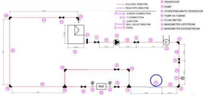
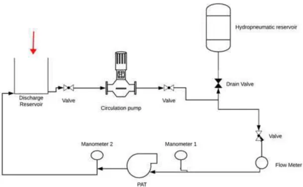
The installation has a discharge reservoir where water is drained to the circuit through a pump, next an hydropneumatic reservoir or RCA (Reservoir of Compressed Air) to stabilize the output pressure of the pump. Then the PAT is tested. There are also measurement elements in the system in order to monitor flow and pressure. The detailed schematic is shown in figure 3.1.

Figure 3.1: Design Experimental Unit

Only steady-state will be considered in this thesis. However, transient electrical and hydraulic analysis is extremely important in order to design appropriate electrical protection methods.

3.1.1 System Design Parameters

In order to start the design of the test rig some parameters were pre-defined. Selection of pumps, reservoir and measurements devices are dependent on the definition of such parameters.

The test rig intends to simulate the conditions of a water distribution network, as a way of verifying the possibility of energy production. Due to this fact the parameters of a WDN were assumed in the first place.

1. Type of water system: Clean water without waste;

2. Available head: 4 m;

4. Pipe diameter: DN50 (50 mm);

5. Maximum Pressure: PN10 (10 bar).

The pre-selected PAT has the operation point of (3.4 L/s, 4 m), which will be the design system point, it is equivalent to a site location in hydropower design where there is an available head and flow for energy production.

3.1.2 Pipe Design

In order to make the hydraulic design of the system it is necessary to consider the effect

of dissipative forces, head losses. In this case, that will allow the calculation of the net head. The design net head, see equation 3.1, will be used to define the design output of a turbine, in this case the PAT (using the maximum power output for the best efficiency

head).

H0=Zu Zd

X

i ∆_H

i (3.1)

whereZu is the water level intake,Zd is the water level tailace and∆Hiare all the head

losses, both variables are expressed in m.

There are also losses along pipes (friction head losses and singular losses). It is possible to assess the effect of losses in pressure drop after their calculation. The type of loss

depends on pipe topology. In a closed pressurized system the velocity is high enough to ensure uniform turbulent flow. So in this situation the flow type is turbulent (Re > 2,000) and Colebrook-White formula (explained ahead) must be used for friction head loss calculation, with an iterative method to solve the friction factor for each discharge value. However, Moody diagram allows a graphical calculation knowing:V (mean velocity),D

diameter,krabsolute roughness and⌫kinematic viscosity of water.

Flow losses will increase with the square of flow velocity. And the flow loss is given by the sum of constituent pipelines parts friction loss and local losses from all components and fittings.

• Friction head loss

As presented before, Bernoulli’s equation allows the calculation of a fluid flow. The equation uses as principle the first law of thermodynamics (the energy in an isolated system

is constant; energy can be transformed but never destroyed) and it calculates the energy

balance of an incompressible flow in steady state. Equation 3.2 is the general equation for head losses, in circular pipes.

hL=∆

✓_p

⇢+z+

V2

2g

◆

wherehLis the head loss, expressed in m;pis the pressure drop, expressed in Pa;zis

the pipe elevation, expressed in m;V the average flow velocity, expressed in m/s;gis the

acceleration of gravity, expressed in m/s2_.

Along a canal or a penstock the friction loss is expressed by equation 3.3, withJbeing

the hydraulic gradient andLthe length of the canal or penstock, expressed in m. Using

equation 3.3 and Darcy-Weisbach factor (equation 3.4) it is possible to define the friction head loss equation 3.5.

∆_H

r=JL (3.3)

f = JDint

V2/2g (3.4)

hr=f

L

D_intV_2g2 (3.5)

Mean velocity (V) is defined as the average velocity of flow across a section (determined

by the continuity equation for steady state flow). It is expressed as a ratio between volumetric flow rate (Q) m3/s and radius-sectional inlet section (S_inlet) m2of the pipe, as shown in equation 3.6. The cross section in the pipe is defined by equation 3.7. The inlet diameter of a pipe is calculated using the thickness of the pipe (e), see figure 3.2 and

equation 3.8.

V = Q

S_inlet (3.6)

Sinlet=⇡r2=

⇡D_inlet2

4 (3.7)

Figure 3.2: Calculation of inlet diameter

Dinlet=Doutlet 2e (3.8)

As mentioned before, the design formula for turbulent friction is expressed by Colebrook White formula 3.9 in which✏represents the wall absolute roughness, equation 3.10 is

the relative roughness ratio. This ratio indicates the roughness ratio of a pipe or tube; an high value of this ratio indicates a larger friction factor that leads to an higher pressure drop. Roughness ratio can be calculated using Moody’s Diagram, see figure3.3, or the recommended table values (table 3.1).

1

f1/2 = 2log ✓_✏/d

3.7 +

2.51 Redf1/2

◆

(3.9)

kr= ✏

D[mm] (3.10)

Re=V D

⌫ (3.11)

Figure 3.3: Moody Diagram

Singular or Local losses

Table 3.1: Surface roughness (k) for pipes

Pipe material New pipe

k(mm)

Old pipe

k(mm)

plastic 0.01 0.25

drawn steel 0.05 1.0

welded steel 0.1 1.0

drawn stainless steel 0.05 0.25

welded stainless steel 0.1 0.25

cast iron 0.25 1.0

galvanizes steel 0.15

cause additional losses that compromise both friction and turbulent components. The generic equation for single head loss can be calculated using equation 3.12, ⇣ is the coefficient of singular loss that depends on the geometry of the singularity of the network

and Reynolds number. Each element of the network will have a specific value for single loss, table 3.3 and appendix I. Usually, the values, specially for valves, are determined experimentally and the data must be provided by manufactures. It is important to note that friction loss of these elements are not included in the local resistance factor, instead this factor is calculated as a part of the main friction loss by including their length and diameter when calculating the pipeline length.

hs=⇣

V2

2g (3.12)

where,V is the velocity andgis the gravity acceleration.

Table 3.2: Pipe Bend: Local losses coefficient_⇣

Element ⇣

Pipe Bend 90, R/D=1.5 0.3

Discharge Loss 1 (pipe without expansion) Swing Check Valve 1....2

Ball Check Valve 0.7 ... 1.2

Gate Valve 0.2

Table 3.3: Tee: Local losses coefficient_⇣

Tee

Qh/Q _⇣↵= 90

s ⇣h

0.8 0.72 0.51

1.0 0.91 0.6

pipe length must match the pump’s region of maximum efficiency.

hpump=

Power

⇢gQ =hf =f L d

V2

2g (3.13)

There are two types of measurement units commonly used for pipelines, inches and millimetres, table 3.4.

Table 3.4: Nominal diameters millimetres vs inches

DN mm in

25 1”

32 1 1/4”

40 1 1/2”

50 2”

Using the system design presented in figure3.1, total head loss is 5.6 meters, table 3.5.

Table 3.5: Total Head loss

Type of loss Value Regular 2.9 m Singular 2.7 m

TOTAL 5.6 m

3.1.3 Machines Design: PAT and Pump

As described before, the PAT was pre-selected in order to have the operation point (3.4 L/s, 4 m), given by pump curve, figure 3.4 and annex IV. Although, to design the initial pump (responsible for the water circulation through the pipelines) it was necessary to consider a pump curve having as guide principle the pipe head loss, the pump selection must correspond to at least a 10 meters head, because of the sum head loss of plus 4 meters head loss of PAT.

In order to achieve the requirements, a pump with a maximum of 20 meters head was pre-selected, figure 3.5 (Curve C) and annex V.

Information about the selected induction machine can be found in annexVI.

Figure 3.4: PAT Curve