A study of simulated annealing variants
Ana I.P.N. Pereira
1, Edite M.G.P. Fernandes
21[email protected], Braganca Polytechnic Institute, Braganca, Portugal 2[email protected], Minho University, Braga, Portugal
Abstract
Este trabajo presenta un estudio comparativo de cinco variantes del método simulated annealing de optimización global. Con la nueva vari-ante aquí propuesta (ASALO), se obtiene el mejor valor de la función y un mayor porcentaje de convergencias.
Keywords: Global optimization; simulated annealing.
1.
Introduction
Consider the nonlinear optimization problem in the following mathema-tical form:
max
t∈T g(t) (1)
whereg:IRn→ IR is a given nonlinear function andTis a compact set dened byT ={t∈IRn :ai≤ti≤bi, i= 1, ..., n}. A global solution to problem (1) is
the pointt∗∈T such that∀t∈T, g(t∗)≥g(t).
There are two types of numerical methods to solve this problem. The deterministic methods usually require a great deal of information and condi-tions on the objective function and they do no guarantee convergence to the global maximum. On the other hand, the stochastic methods can be easily implemented and converge in practice to a global maximum. In particular, for the simulated annealing method, it has been proved that it converges asymp-totically to a global solution.
Examples of stochastic methods are: Multistart, clustering, multi level, adaptive random search, genetic algorithms and simulated annealing.
Motivated by analogy with the behavior of physical systems in the pres-ence of a heat bath, Kirkpatrick, Gelatt and Vecchi (1983), and Cerny (1985), proposed the simulated annealing (SA) approach to solve combinatorial opti-mization problems. Since then, the SA algorithm has been applied in many areas such as the graph partitioning, graph coloring, number partitioning, cir-cuit design, composite structural design, data analysis, image reconstruction, neural networks, biology, geophysics and nance [7, 10, 15].
In this paper, we describe ve variants of the simulated annealing method and analyze their performances for a standard set of test functions. This paper is organized as follows. Section 2 describes the simulated annealing algorithm and the four crucial phases of the method. In Section 3 we present ve variants of the simulated annealing method including the new ASALO variant. The numerical results are shown in Section 4 and Section 5 contains the conclusions.
2.
Simulated Annealing method
In 1953, Metropolis et al. proposed an algorithm to simulate the be-havior of physical systems in the presence of a heat bath. Thirty years later, Kirkpatrick et al. [11] applied the Metropolis algorithm to combinatorial opti-mization problems and named it by simulated annealing.
In 1986, Bohachevsky et al. [1] applied the SA algorithm to solve con-tinuous optimization problems. Since then, the SA algorithm has been subject to various modications in order to improve its eciency. See, for example, Corana et al. [2], Dekkers and Aarts [3], Ingber [8], Romeijn and Smith [14] and Szu and Hartley [16].
The spread use of the SA algorithm is mainly due to the fact that it is easily implemented, it can be applied to any optimization problem, it does not use any derivative information, it does not require specic conditions on the objective function and it has been proved that the SA algorithm asymptotically converges to a global maximum.
2.1. The SA algorithm
The SA algorithm can be easily described using four phases: the gener-ation of a new candidate point, the acceptance criterion, the reduction of the control parameter and the stopping criterion.
Algorithm 2.1 Given an initial approximationt0, a control parameterc0 and
the number of iteration with the same control parameterNk c
while stopping criterion is not reached do for j= 1toNk
c do
Generate a new candidate pointy Analyze the acceptance criterion end
UpdateNk c
The remaining of this section is devoted to present in detail the four referred phases of the SA algorithm.
2.2. Generation of a new candidate point
The generation of a new candidate point is one of the crucial phases of the SA algorithm. Obviously, the scheme that is used to generate a new point aects the performance of the algorithm. This scheme must be such that a good exploration of the search region and a feasible point are provided.
The initial approximation,t0, is usually randomly generated. However,
some authors suggest that this initial approximation should be constructed throughout a preliminary analysis of the problem.
Then, a new point is found using the current approximation, tk, and
the generating probability density function,ftky(ck). This function establishes
how the new candidate point is created and usually depends on the control parameterck and/or on the dimension of the problem.
Techniques to generate new candidate points can be found in the fol-lowing papers: Bohachevsky et al. [1], Corana et al. [2], Dekkers and Aarts [3], Ingber [8], Romeijn and Smith [14], Szu and Hartley [16] and Tsallis and Stariolo [17].
2.3. Acceptance criterion
The acceptance criterion allows the SA algorithm to avoid getting stuck in local, non-global maximum, when searching for global maximum. This is accomplished by accepting points where a decrease of the objective function is veried. During the process, the probability of negative movements decreases slowly to zero and in the nal phase, the algorithm improves the precision of the approximation to a global maximum.
Atky(ck)is the acceptance function and it represents the probability of
accepting the pointy whentk is the current point. This function depends on
the control parameter and on the dierence of the function values at the points y andtk. The acceptance criterion has the following form
tk+1=
½
y if τ ≤Atky(ck)
tk otherwise
where tk is the current approximation to the global maximum, y is the new
candidate point andτ is a uniformly random number drawn from U(0,1).
WhenAtky¡ck¢= min
(
1, e−
g(tk)−g(y)
ck
)
This criterion accepts all points where the objective function value in-creases, i.e.,f(tk)≤f(y), becausee−f(tk)−f(y)
ck ≥1. However, iff(tk)> f(y),
the pointy might be accepted with some probability.
When the control parameterckis high, the maximization process searches
in all feasible region, looking up for promising regions to nd the global maxi-mum. As the algorithm develops,ckis slowly reduced and the process computes
best approximations to a optimum.
The Metropolis criterion is the most used acceptance criterion in all the SA variants. In particular, this criterion is used in all variants presented in the Section 3. Dierent acceptance criteria are suggested in the literature. See Ingber [8] and Tsallis and Stariolo [17] papers.
2.4. Reduction of the control parameter
The function ck is called the control parameter, temperature or cooling
schedule, and must be a decreasing function that veries
lim
k→∞c
k = 0.
A crucial phase of the SA algorithm is to determine how the control parameter should be reduced. The procedure must be quick and guarantee that the SA algorithm converges to a global maximum.
For a good performance of the algorithm, the initial control parameter must be suciently high (to search for promising regions) but not extremely high because, in this case, the algorithm becomes too slow. To solve this dilemma, some authors suggested that a preliminary analysis of the objective function should be done in order to get an appropriate value, Dekkers and Aarts [3], Ingber [8] and Laarhoven and Aarts [12].
2.5. Stopping criterion
Any iterative process requires a stopping criterion to terminate the al-gorithm. There are in the literature many stopping criteria that can be used to terminate de SA algorithm. All criteria are based on the idea that the algo-rithm should terminate when "... the system "freezes" and no further changes occur..."[11]. The usual stopping criterion is to limit the number of function evaluations (later denoted in the paper by NF E_M AX). Other used
stop-ping criterion denes a lower limit for the value of the control parameter. In this case, the iterative process terminates when the control parameter veries ck < c
min, wherecmin is a pre-dened parameter.
i.e, the algorithm stops if the following condition is veried forN∗ successive iterations
|f∗−fant∗ |< ε wheref∗
antrepresents the previous approximation to an optimum value.
Dier-ent termination criteria were proposed by Corana et al. [2], Dekkers and Aarts [3] and Ingber [8].
3.
Variations on original simulated annealing
To accelerate the convergence of the SA algorithm many variants have been appeared in the literature. In this section we describe ve variants of the simulated annealing method: the standard simulated annealing, herein denoted by SSA, the variant of the SA algorithm presented by Corana et al. (CSA), the ASA variant suggested by Ingber, the SALO algorithm proposed by Desai et al. and our variant, named ASALO algorithm, which combines some ideas from the ASA and SALO variants.
3.1. Standard SA variant
The standard simulated annealing (SSA) or Boltzmann annealing algo-rithm for continuous optimization was proposed by Bohachevsky et al. [1]. In this algorithm, the generation of a new candidate point is based on the cur-rent approximation and on a direction vector. The new point is computed by y=tk+λ.
The control parameterck decreases through the reduce factorµby the
following way
ck+1=µkck
where the reduce factorµ∈(0,1). In the SSA algorithm theNk
c is constant.
3.2. Corana SA variant
In 1987, Corana et al. [2] suggested one variant of the simulated anneal-ing algorithm (CSA). Later, Goe et al. [5] proposed some modications to the CSA algorithm.
This variant consists of using adaptive moves along the coordinate di-rections. For that, each new candidate point is obtained through the cur-rent approximation changing only one coordinate. The new point is given by y=tk+dk
iλkiei, wheredki is a uniformly distributed random variable in(−1,1),
λk
i is the component of the step vectorλk andeiis the euclidian vector. After
Nλ iterations, each step vector componentλki is updated to better adjust the
optimization problem. The valuedk
i is given bydki = 2u−1whereuis a uniformly distributed
as follows
λki =
λk i ∗
£
1 +Vi∗(r−0.40.6)
¤
0.6< r λk
i 0.4≤r≤0.6 λki
[1+Vi∗(0.04.−4r)]
r <0.4
where rrepresents the percentage of points accepted according to the coordi-nate i, i.e.,r= (number of the accepted points according to coordinatei)/(Nλ)
andVi is a xed value throughout the process.
The main idea for this adjustment is to accept 50% of the generated points. To accomplish this, the algorithm proceeds as follows: if 0.6< r then more than 60% of generated points were accepted. This behavior indicates that the generated points are far away from the global maximum. In this situation, theith coordinate of the step vector should proportionally increase according to the factorη∈(1,1 +Vi]. On the other hand, if the algorithm accepted less
than 40% of the generated points, then the ith coordinate of the step vector should proportionally decrease according to the factorη ∈h1+V1 i,1´. Finally,
when the algorithm accepted between 40 % and 60% of the generated points, then the step vector should not be updated.
Goe et al. suggested that the number of the iteration with the same control parameter value should be constant during the process [5].
3.3. ASA variant
Ingber [6], in 1989, introduced some alterations to the Fast Annealing algorithm proposed by Szu and Hartley, and named it by Very Fast Simu-lated Annealing. Later, in 1993, Ingber [7] renamed it by adaptive simuSimu-lated annealing (ASA) and it is the most used variant of the SA method today.
This variant is characterized by two functions: the generating probability density function, ftky(cG), and the acceptance function, Atky(cA). The rst
function determines how a new candidate point is generated and the second one establishes if a candidate point is accepted. Both functions depend on the current approximation, on the new candidate point and on the control parameters,cG∈IRn andcA∈IR, respectively.
Algorithm 3.1 (ASA) Given a initial feasible approximation t0, k
A=kG =
0, κ=−ln [ǫ]e−ln[nN ǫ], the control parametersc0
A,c0Gi = 1.0 and the number of
iterations for reannealingNA_max
ifnA≥NA_max then redene kA andkG
Reduce the control parameter end
Motivated by the fact that the objective function behaves dierently along dierent directions, Ingber proposed dierent generating probability den-sity functions for dierent variables. So,firepresents the generating probability
density function associated with theti variable, and it is given by
fi
¡
tki, λi, ckGi
¢
= 1
2£
|λi|+ckGi
¤
ln
µ
1 + ck1 Gi
¶ for 1≤i≤n.
A new candidate point,y= [y1, ..., yn], is determined as follows
yi=tki +λi(bi−ai) for1≤i≤n (2)
whereaiandbiare the lower and upper bounds for thetivariable, respectively.
The valueλi∈(−1,1)is given by
λi=sgn
µ
u−1
2
Ã
1 + 1
ck Gi
!|2u−1| −1
ckGi (3)
whereuis a uniformly distributed random variable in(0,1).
Wheny is not a feasible point, then a new candidate point is computed using equations (2) and (3).
It is possible in this variant to redene the control parametersck Gi and
ck
A in order to speed up the search process. AfterNA_maxaccepted points, the
sensitivities given by
si=
¯ ¯ ¯ ¯
g(t∗+δt∗
iei)−g∗
δt∗ i ¯ ¯ ¯ ¯
are computed, wheret∗is the best point found so far,δis a small real parameter andei∈IRn is the euclidian vector. Let
smax= max 1≤i≤n{si},
then the parameterkGi is updated by
kGi=
· −1 κln µ smax si
ckGi c0
Gi
¶¸n
if smax si
ckGi c0
Gi <1
wherec0
Gi is the initial value of the control parametercGi.
Similarly, the parametersc0
A andkA are redened using
c0A= min
©
c0A,max
©¯ ¯g
¡
tk¢¯ ¯,|g∗|,
¯ ¯g
¡
tk¢ −g∗¯
¯ ªª
and
kA=
· −1 κln µ ¯ cA c0 A ¶¸n
wherec¯A= min
©
c0A,max
©¯ ¯g
¡
tk¢
−g∗¯¯, ckA ªª
.
The value κdepends on ǫandNǫ. This parameter is dened by
κ=−ln [ǫ]e−ln[nN ǫ]
where the valuesǫandNǫ should be such that
½
cfGi =c0 Giǫ
kf =N ǫ
with cfGi, the nal value of the control parameter cGi, and k
f represents the
maximum number of iterations allowed. The inuence of the values ǫandNǫ
in the algorithm can be analyzed in Niu [13]. In this algorithm, the size of the chain is one, meaning that the control parameter is always updated as follows
(
kGi =kGi+ 1
ck Gi=c
0 Gie
−κ(kGi)n1 for1≤i≤n.
Similarly, the control parameter associated with the acceptance function is updated by
(
kA=kA+ 1
ck
A=c0Ae−κ(kA) 1
n
wherec0
Arepresents the initial value of the control parametercA. Ingber ensures
that, statistically, the algorithm determines a global maximum of the initial problem. We refer to [6, 8, 9] for more details.
3.4. SALO variant
Desai and Patil [4] suggested the variant SALO that combines the ASA algorithm with a local search procedure. SALO variant is similar to the ASA variant except in the generation of the new candidate point, where a local search algorithm, named hill climber, is used.
So, given a current approximationtk, a slight perturbation is carried out
based on the initial approximation y¯k+1 and the resulting point is the new
candidate point for SA method,y.
This procedure generates a sequence of local maxima of the initial prob-lem,{tk}. Desai and Patil guarantee that SALO variant converges, with
prob-ability one, to a global maximum of the optimization problem. 3.5. ASALO variant
In practice, some variants of the SA algorithm converge to an approxima-tion that might not be suciently close to the global maximum. Our purpose is then to improve the precision of the approximation to a global maximum as well as to reduce the execution time. We propose herein the ASALO variant that is based on ASA and SALO algorithms and contains some strategies sug-gested by Romeijn and Smith [15] to guarantee that the generated points are feasible.
The determination of infeasible points causes an expense of execution time. For this reason, our ASALO variant incorporates a reection technique proposed by Romeijn and Smith which can be summarized as follows.
Given a point y¯ = [¯y1, ...,y¯n], the new candidate point is obtained by
applying the following function to each coordinate of the pointy¯
r(¯yi) =
ai+ (ai−y¯i) if y¯i< ai
¯
yi if ai≤y¯i≤bi
bi−(¯yi−bi) if y¯i > bi
.
The new candidate, in ASALO variant, is then the pointy= [r(¯y1), ..., r(¯yn)].
If this point is accepted, a local search procedure is implemented withy as the initial approximation. The resulting point of the local search procedure is the new approximation to the global maximum.
4.
Computational Results
The ve previously presented variants were implemented in C on a Pen-tium II, Celeron 466 Mhz with 64Mb of RAM. For the computational expe-riences we considered eight test functions (Branin (B), Goldstein and Price (GP), Shubert (S), Rosenbrock (R2 e R4), sphere model (M e3), Hartmann
(H3) and Rastrigin (Ra4)). Each variant was run four times for each test
func-tion with dierent random initial approximafunc-tions. The following results are the average of the obtained numerical results in the successful runs.
We choose to use the following values. In the stopping criterion:N∗= 5, ε= 10−6,N
F E_M AX = 100000andNF E_M IN = 1000. For the CSA variant,
we consideredVi = 2.0andλi0= 1.0fori= 1, ..., n(as suggested by Corana et
the SSA and CSA variants: µ= 0.95andNk
c=21. In ASA, SALO and ASALO
variants, we usedǫ= 10−5 andN
ǫ= 100.
To determine the initial control parameter value, c0, (or c0
A in ASA,
SALO and ASALO variants) a preliminary analysis for each test function was carried out. For that, we considered a sample of10×nfeasible points (where nrepresents the dimension of the problem), and tested Dekkers and Aarts [3], Laarhoven and Aarts [12] and Ingber [8] proposals. Dekkers and Aarts proposal provided the best results.
4.1. Characterization of the presented variants
Some tests were done to characterize the presented variants. This study aims to identify the parameters that most inuence the behavior of the pre-sented variants.
The SSA and CSA variants have similar behavior and the crucial param-eters in these variants areµandc0values. Ifµhas a value near 1 then the
se-quence{ck}slowly decreases to zero and consequently the initial control
param-eter must be small. Two cases were analyzed: µ= 0.995andc0=min{1.5,c¯}
wherec¯is the value obtained by a preliminary analysis;µ= 0.95and the initial
control parameter is determined by a preliminary analysis.
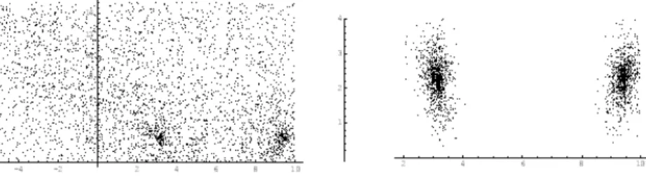
Figure 1 shows the accepted points provided by the SSA variant on the Branin test function for both cases. In the rst, the initial control parameter at the beginning of the process has a high value and SSA variant behaves like a random method.
Figure 1: Accepted points in SSA algorithm
In all performed tests we veried that when µ = 0.995 then c0 = 1.5.
high. In this case, the initial control parameter is a small value and the SSA variant only accepts points close to the global maxima, as shown in Figure 1.
When the test function has more than one global maximum, the SSA variant was able to identify them.
Based on the same type of tests, identical conclusions can be drawn for the CSA variant.
For ASA, SALO and ASALO variants, we veried that c0, ǫ and Nǫ
parameters are the ones that most inuence the performance of the algorithms. In all tests, these variants have similar behavior: they rapidly converge to a point and provide a good approximation to an optimum.
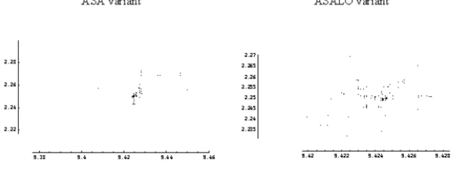
Figure 2 presents the accepted points obtained by ASA and ASALO variants for the Branin test function.
Figure 2: Accepted points in ASA and ASALO algorithms
We can see that these variants concentrate the search on the promising region of a global maximum. We also found that the ASA, SALO and ASALO variants quickly identify one promising region and that most of the accepted points are used to improve the precision of the approximation to a global max-imum. However, we point out that these variants usually nd only one global maximum.
4.2. Comparison of the presented variants
The computational experiences were mainly carried out to identify ro-bustness, eciency and the precision of the approximations to the global max-imum.
of function evaluations NF E, number of the accepted points NAP, the nal
function average valueg∗
m and the best nal function value foundg∗. When (#) appears before the number of function evaluations, it means that#is the
number of runs (out of 4) that did not converge to a global maximum. In these cases, the variant provided a local maximum.
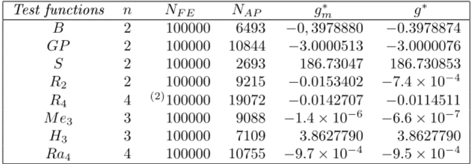
In Tables 1 and 2 we present the obtained numerical results for SSA and CSA variants.
Test functions n NF E NAP gm∗ g∗
B 2 100000 6493 −0,3978880 −0.3978874
GP 2 100000 10844 −3.0000513 −3.0000076
S 2 100000 2693 186.73047 186.730853
R2 2 100000 9215 −0.0153402 −7.4×10⁻⁴
R4 4 (2)100000 19072 −0.0142707 −0.0114511
M e3 3 100000 9088 −1.4×10⁻⁶ −6.6×10⁻⁷
H3 3 100000 7109 3.8627790 3.8627790
Ra4 4 100000 10755 −9.7×10⁻⁴ −9.5×10⁻⁴
Table 1: Results of four runs of SSA algorithm
Test functions n NF E NAP g∗m g∗
B 2 24402 9435 −0.3978874 −0.3978874
GP 2 33769 15489 −3 −3
S 2 23562 5694 186.730909 186.730909
R2 2 100000 23240 −0,0241800 −8.4×10⁻⁴
R4 4 (1)72762 28109 −0,0217699 −0,0011088
M e3 3 34587 13603 −6.3×10⁻⁸ −1.5×10⁻⁸
H3 3 26565 10812 3,86277820 3,8627821
Ra4 4 46452 16209 −1.4×10⁻⁷ −2.6×10⁻⁸
Table 2: Results of four runs of CSA algorithm
The SSA variant requires a high number of function evaluations always reaching the maximum value allowed. This fact indicates that the variant in-tensely searches on the feasible set. In problem R4, two runs converge to a
local maximum. The CSA variant requires a smaller number of function eval-uations and provides better approximations to the global maximum. However, as expected, it accepts more points than the SSA variant. This increase in the number of accepted points improves the precision of the approximations to a global optimum.
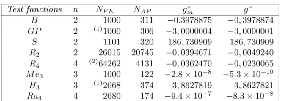
Test functions n NF E NAP g∗m g∗
B 2 1000 311 −0.3978875 −0,3978874
GP 2 (1)1000 306 −3,0000004 −3,0000001
S 2 1101 320 186,730909 186,730909
R2 2 26015 20745 −0,0394671 −0,0049240
R4 4 (2)64262 4131 −0,0362470 −0,0230065
M e3 3 1000 122 −2.8×10⁻⁸ −5.3×10⁻¹⁰
H3 3 (1)2068 374 3,8627819 3,8627821
Ra4 4 2680 174 −9.4×10⁻⁷ −8.3×10⁻⁸
Table 3: Results of four runs of ASA algorithm
Test functions n NF E NAP gm∗ g∗
B 2 43271 322 −0,3978874 −0,3978874
GP 2 50004 281 −3,0000002 −3
S 2 53016 318 186,730908 186,730909
R2 2 43363 203 −2.8×10⁻⁶ −1.3×10⁻⁷
R4 4 (2)100000 188 −0.0397128 −0.0199250
M e3 3 40221 87 −1.7×10⁻⁸ −4.7×10⁻¹¹
H3 3 67699 296 3,8627814 3,8627820
Ra4 4 79033 96 −2.4×10⁻⁶ −2.9×10⁻⁷
Table 4: Results of four runs of SALO algorithm
When we compare these results with the CSA variant results, we may conclude that ASA variant does not improve the precision of the approxima-tions. However, the ASA variant drastically reduces the number of function evaluations and of accepted points.
In some problems, SALO variant provides better approximations to a global maximum than the previous variants. This was already expected since this variant incorporates a local search procedure. In terms of accepted points, ASA and SALO have similar behavior, except for the problems R2 and R4
where SALO variant has the better results. Due to the local search procedure, SALO variant requires a high number of function evaluations. ASA variant is very fast to identify the region where a maximum is, so needing a fewer number of function evaluations. This is probably the reason why the ASA variant is not able to identify the global maximum and converges to a local one.
Finally, Table 5 presents the numerical results obtained by the ASALO variant.
Test functions n NF E NP A gm∗ g∗
B 2 15531 284 −0,3978874 −0,3978874
GP 2 15944 285 −3 −3
S 2 21527 374 186,730907 186,730909
R2 2 16671 294 −2.8×10⁻⁶ −8.8×10⁻⁸
R4 4 (1)40923 577 −0,0265422 −0,0049288
M e3 3 5717 98 −4.0×10⁻⁹ −2.6×10⁻¹¹
H3 3 15237 260 3,8627815 3,8627821
Ra4 4 10293 143 −1.6×10⁻⁶ −5.5×10⁻⁸
Table 5: Results of four runs of ASALO algorithm
When compared with ASA, the ASALO variant needs more function evalua-tions although fewer than the remaining variants. In terms of accepted points, ASA, SALO and ASALO variants have similar behavior. Of all the presented variants, SALO and ASALO were the best ones as far as the number of accepted points is concerned.
The ASALO and CSA variants obtained so far the best approximations to the global maximum. In particular, the CSA variant gives better results than ASALO variant in two test function,R2 andR4. In the other test functions,
ASALO variant produces better or equal approximations than the remaining variants. ASALO and CSA variants reached the best nal function average value and both have only one run that does not converge to a global maximum. Besides ASA, the ASALO variant also requires a small number of function evaluations.
5.
Conclusions
We propose a new variant of the SA algorithm, herein denoted by ASALO, combining the adaptive simulated annealing and a local search procedure with a reection technique which aims to generate feasible points. The new algorithm, together with other four well-known variants of the SA algorithm were tested with a set of standard test functions in order to analyze their performances.
The numerical results indicate that the variants that are more eective, in terms of number of function evaluations, are ASA and ASALO. When we compare the number of accepted points, ASA, SALO and ASALO variants have similar behavior. The ASALO variant provides the best maximum function value. When the problem has more than one global optimum, SSA and CSA were able to recognize more than one solution. However, ASA, SALO and ASALO variants usually identify only one solution.
than one global maximum have to be identied. If only one global maximum is requested, than ASA is more ecient as far as the number of function eval-uations is concerned. To obtain the best function value and a high percentage of solved problems, the ASALO variant seems slightly superior.
6.
Bibliography
[1] Bohachevsky, I. O., Johnson, M. E. and Stein, M. L. (1986). Generalized Simulated Annealing for Function Optimization. Technometrics 28, no. 3, 209-217.
[2] Corana, A., Marchesi, M., Martini, C. and Ridella, S. (1987). Minimizing Multimodal Functions of Continuous Variables with the simulated Anneal-ing Algorithm. ACM Transactions on Mathematical Software 13, no 3, 262-280.
[3] Dekkers, A. and Aarts, E. (1991). Global Optimization and Simulated An-nealing. Mathematical Programming 50, 367-393.
[4] Desai, R. and Patil, R. (1996). SALO: Combining Simulated Annealing and Local Optimization for Ecient Global Optimization. Proceedings of the 9th Florida AI Research Symposium FLAIRS - 96, 233-237.
[5] Goe, W. L., Ferrier, G. D. and Rogers, J. (1994). Global Optimization of Statistical Functions with Simulated Annealing. Journal of Econometrics 60, 65-99.
[6] Ingber, L. (1989). Very Fast Simulated Re-Annealing. Mathematical and Computer Modelling 12, no. 8, 967-973.
[7] Ingber, L. (1993). Simulated Annealing: Practice versus Theory. Mathe-matical Computer Modelling 18, no. 11, 29-57.
[8] Ingber, L. (1996). Adaptive Simulated Annealing (ASA): Lessons Learned. Control and Cybernetics 25, no. 1, 33-54.
[9] Ingber, L. and Rosen, B. (1992). Genetic Algorithms and Very Fast Simu-lated Reannealing: A Comparison. Mathematical Computer Modelling 16, no. 11, 87-100.
[10] Johnson, D. S., Aragon, C. R., McGeoch, L. A. and Schevon, C. (1991). Optimization by Simulated Annealing: An Experimental Evaluation; part II, graph coloring and number partitioning. Operations Research 39, no. 3, 378-406.
[12] Van Laarhoven, P. J. M. and Aarts, E. H. L. (1987). Simulated Anneal-ing: Theory and Applications. Mathematics and Its Applications. Kluwer Academic Publishers.
[13] Niu, X. (1999). An Integrated System of Optical Metrology for Deep Sub-Micron Lithography. Ph.D Thesis. University of California.
[14] Romeijn, H. E. and Smith, R. L. (1994). Simulated Annealing for Con-strained Global Optimization. Journal of Global Optimization 5, 101-126. [15] Romeijn, H. E., Zabinsky, Z. B., Graesser, D. L. and Neogi, S. (1999). New Reection Generator for Simulated Annealing in Mixed-Integer/Continuous Global Optimization. Journal of Optimization Theory and Applications 101, no. 2, 403-427.
[16] Szu, H. and Hartley, R. (1987). Fast Simulated Annealing. Phys Lett A 122, no. 3-4, 157-162.