www.ann-geophys.net/29/97/2011/ doi:10.5194/angeo-29-97-2011
© Author(s) 2011. CC Attribution 3.0 License.
Annales
Geophysicae
Inductive ionospheric solver for magnetospheric MHD simulations
H. Vanham¨aki
Arctic Research Unit, Finnish Meteorological Institute, Helsinki, Finland
visiting at: Solar-Terrestrial Environment Laboratory, Nagoya University, Nagoya, Japan
Received: 29 March 2010 – Revised: 12 August 2010 – Accepted: 29 December 2010 – Published: 10 January 2011
Abstract. We present a new scheme for solving the iono-spheric boundary conditions required in magnetoiono-spheric MHD simulations. In contrast to the electrostatic ionospheric solvers currently in use, the new solver takes ionospheric induction into account by solving Faraday’s law simultane-ously with Ohm’s law and current continuity. From the view-point of an MHD simulation, the new inductive solver is similar to the electrostatic solvers, as the same input data is used (field-aligned current [FAC] and ionospheric conduc-tances) and similar output is produced (ionospheric electric field). The inductive solver is tested using realistic, databased models of an omega-band and westward traveling surge. Al-though the tests were performed with local models and MHD simulations require a global ionospheric solution, we may nevertheless conclude that the new solution scheme is feasi-ble also in practice. In the test cases the difference between static and electrodynamic solutions is up to∼10 V km−1 in certain locations, or up to 20-40% of the total electric field. This is in agreement with previous estimates. It should also be noted that if FAC is replaced by the ground magnetic field (or ionospheric equivalent current) in the input data set, exactly the same formalism can be used to construct an in-ductive version of the KRM method originally developed by Kamide et al. (1981).
Keywords. Ionosphere (Electric fields and currents) – Magnetospheric physics (Magnetosphere-ionosphere inter-actions)
Correspondence to:H. Vanham¨aki ([email protected])
1 Introduction
Magnetospheric magnetohydrodynamic (MHD) simulations are used extensively in studying the near-earth plasma en-vironment, its inner dynamics and coupling with the solar wind. In addition to the magnetospheric (ideal) MHD model, simulations also require a separate ionospheric solver that provides inner boundary conditions for the magnetospheric solution.
It would appear that at the present time global MHD sim-ulations use electrostatic solvers in the ionosphere (e.g. Jan-hunen, 1996; Raeder et al., 1998; Tanaka, 2000; Lyon et al., 2004, and references therein), meaning that inductive effects are ignored and the ionospheric electric field can be repre-sented by a potential. Janhunen (1998) considered a type of electrodynamic solver where the ionospheric electric field may contain a non-potential component. However, even in this approach Faraday’s law is not solved in the ionosphere, for the electric field is obtained by a direct mapping from the magnetosphere.
The electrostatic approximation is usually valid in the ionosphere, because typical current systems evolve rather slowly, in time scales of several minutes. Nevertheless, it has been shown that inductive effects may play an important role in the reflection of Alfv´en waves at the ionospheric boundary (e.g. Yoshikawa and Itonaga, 1996; Buchert, 1998; Lysak and Song, 2001). More recently Vanham¨aki et al. (2007) showed that in very dynamical situations, like in a westward traveling surge, induction may contribute up to 30% of the total elec-tric field in some limited areas. Takeda (2008) concluded that induction may affect rapidly changing, global current sys-tems, such as the preliminary impulse of storm commence-ment. These results suggest that ionospheric induction may have a non-negligible role in magnetosphere-ionosphere cou-pling, especially during active periods such as substorm on-sets.
In this article we present a scheme for an inductive iono-spheric solver, where ionoiono-spheric Ohm’s law, current conti-nuity and Faraday’s law are solved simultaneously and self-consistently. From the viewpoint of an MHD simulation, the inductive solver is quite similar to the existing electrostatic solvers, as the same input data is used (field-aligned current [FAC] and ionospheric conductances) and similar output is produced (ionospheric electric field). However, the structure of the calculated electric field may be different, depending on the temporal evolution of the input data.
We begin by reviewing the electrostatic ionospheric solver presently used in MHD simulations in Sect. 2, together with some proposed alternative schemes. The theory behind the new inductive solver is discussed in Sect. 3, while in Sect. 4 we present some simple applications illustrating the feasibil-ity of the method. Actual implementation of the new induc-tive solver in a magnetospheric MHD simulation is beyond the scope of the present theoretical study. Details of the so-lution algorithm are given in an Appendix.
2 Background
2.1 Electrostatic solver
The spatial grid resolution and time step in MHD simula-tions are limited by the Alfv´en speed (VA= |B|/√µ0ρ) and Courant stability condition, which states that for a stable so-lution the time step must be smaller than the wave travel time across each grid cell. For this reason magnetospheric MHD simulations have an inner artificial boundary (AB), usually around 2–3RE, as closer to Earth the increasing Alfv´en speed would make full MHD solution computationally impractical (however, the linearized MHD wave equation can be solved all the way down to the ionosphere, see e.g. Lysak and Song, 2006; Waters and Sciffer, 2008). Instead, the magnetospheric simulation is coupled to an ionospheric solver by mapping FAC and electric field along magnetic field lines. Here we
give a brief summary of the process, further details are given e.g. by Janhunen (1998).
The FAC distribution is calculated at the AB as
jk= ˆek·∇ ×B/µ0, (1)
whereeˆk is the unit vector in the magnetic field direction. When mapped to the ionospherejkscales with the flux tube cross section. Ionospheric conductivities are calculated us-ing a pre-defined model of solar UV radiation and electron precipitation data estimated from the MHD variables at the AB (see e.g. Raeder et al., 1998; Janhunen, 1996).
The ionosphere is treated as a thin spherical shell, with height-integrated Hall, Pedersen and field-aligned conduc-tances6H,6Pand60, respectively. The ionospheric Ohm’s law is
J=6·E. (2)
HereJ denotes the height-integrated horizontal current and we ignore the parallel component of the electric field. The ionospheric conductance tensor is (e.g. Brekke, 1997, chap-ter 7.12)
6=1 C
606P −606HsinI 606HsinI C6P+6H2cos2I
. (3)
whereI is the inclination angle of the magnetic field (+90◦ at the northern magnetic pole,−90◦at the southern pole) and C=60sin2I+6Pcos2I.
Current continuity means that
∇h·J=jksinI, (4)
where the subscript “h” indicates that horizontal derivatives are calculated. Together with Ohm’s law this gives us an el-liptic differential equation for the ionospheric potential elec-tric fieldE= −∇hφ,
−∇h·(6·∇hφ)=jksinI. (5)
The electric potentialφis mapped along magnetic field lines to the AB, where it is used as a boundary condition for the plasma velocity,
V=E×B/|B|2. (6)
If an estimate of the potential drop between the magneto-sphere and ionomagneto-sphere is made, it can be added toφ. 2.2 Solution based on the electric field
the electric field mapped from the MHD simulation generally has a rotational part.
However, in this approach Faraday’s law is not solved in the ionosphere and the rotational part ofE is probably in-consistent with the time derivate of the magnetic field. So for the purposes of this study the solver suggested by Janhunen (1998) can be considered as electrostatic.
Janhunen (1998) identified two difficulties in this elec-tric field-based solver: (1) mapping non-potential elecelec-tric fields between magnetosphere and ionosphere is fundamen-tally ambiguous and (2) it is difficult to change the FAC at the AB, as it affects the magnetic field inside the simula-tion, not only at the AB. Janhunen (1998) presented possi-ble ways to overcome these difficulties, but nevertheless this approach has not been implemented in existing MHD sim-ulations. The first problem is relevant also in the inductive ionospheric solver presented in Sect. 3 and is discussed there in more detail.
2.3 M-I coupling with Alfv´en waves
In the above magnetosphere-ionosphere coupling schemes it is assumed that the electric potential and FAC are instan-taneously mapped along (dipolar) magnetic field lines be-tween the AB and ionosphere. In a more realistic description changes in the M-I system are transmitted as hydromagnetic Alfv´en waves.
The Alfv´en velocity varies considerably along the mag-netic field line, from a few hundred km s−1in the ionosphere up to 105km s−1at 1–2REaltitude (e.g. Paschmann et al., 2002, Fig. 3.12). Consequently, the two-way travel time be-tween AB and ionosphere could be order of 10 s. This is longer than typical time steps of MHD simulations (espe-cially if sub-cycling is used) and should therefore be included in the ionospheric solver. However, this propagation delay is ignored in the presently used electrostatic solvers discussed above, as well as in the new inductive solver presented in Sect. 3.
Reflection of Alfv´en waves from non-uniformly conduct-ing ionosphere with vertical background magnetic field was treated by Glassmeier (1984). He used the electrostatic ap-proximation, where only shear waves are involved. If induc-tive effects are included, there is a mode conversion between shear and compressional Alfv´en waves (e.g. Yoshikawa and Itonaga, 1996; Buchert, 1998; Lysak and Song, 2001). The mode conversion also depends on the inclination of the back-ground magnetic field (Sciffer et al., 2004). More recently Lysak and Song (2006) and Waters and Sciffer (2008) have developed linearized MHD models of Alfv´en wave propaga-tion and reflecpropaga-tion in the near Earth space.
The prospect of using an inner magnetosphere Alfv´en wave model as an ionospheric solver in a global MHD sim-ulation has been discussed by Yoshikawa et al. (2010). They developed a scheme for extracting the incident wave pat-tern from the MHD fields and updating the boundary
con-dition at the AB using the reflected waves. Yoshikawa et al. (2010) considered only an electrostatic ionosphere (shear wave reflection) with vertical background magnetic field and ignored the propagation delay of Alfv´en waves, but it might be possible to use a similar approach to connect e.g. the 3-dimensional, fully electrodynamic Alfv´en wave model devel-oped by Lysak and Song (2006) to a global MHD simulation. In the ionospheric reflection process both the electric field and FAC are modified, in contrast to the solvers discussed in Sects. 2.1 and 2.2, where eitherjkorEremains fixed. As the FAC is changed in the ionosphere, the problem of magnetic boundary condition at the AB, discussed in Sect. 2.2, applies also to Alfv´enic solvers.
3 Inductive (electrodynamic) solver
In this section we present a new inductive solver for mag-netospheric MHD simulations. The new solver is very sim-ilar to the presently used electrostatic solvers discussed in Sect. 2.1, except that inductive effects are included in the ionospheric solution. While this means that the mapping between AB and ionosphere is still handled in a simplified manner, ignoring the wave propagation aspect of the cou-pling, it should also make the new solver more straightfor-ward to implement in magnetospheric MHD simulations than the Alfv´enic solvers discussed by Yoshikawa et al. (2010) and in the previous section.
The new solver uses the same input data as the electrostatic solver,jkcalculated from the MHD solution and ionospheric conductance estimates. However in this case the electric field has a non-potential part, giving us one additional degree of freedom. We can write the electric field as
E= −∇φ+ ˆer×∇ψ, (7)
whereerˆ is a unit vector in radial direction.
As we have one more unknown function than in the elec-trostatic case, we need one more equation. This is obtained by combining Faraday’s and Ampere’s laws,
∇ ×E= −∂B
∂t , (8)
∇ ×B=µ0j. (9)
Here j is the 3-D volume current, j=δ(r−RI)J+jkˆek,
whereRIis the radius of the ionospheric shell.
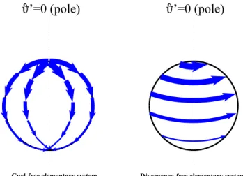
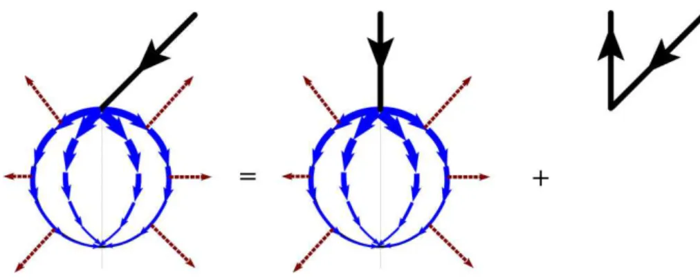
Fig. 1. Curlf-free (left) and divergence-free (right) Spherical Ele-mentary Current Systems (SECS). Figure provided by O. Amm.
3.1 SECS-based solution algorithm
Instead of the potentialsφandψ used in Eq. (7), we may equally well represent the electric field in terms of its diver-gence and curl (we only need the radial component of curl, as we use the thin shell approximation). The Spherical Elemen-tary Current Systems (SECS) introduced by Amm (1997) of-fer a set of convenient basis functions for this kind of repre-sentation.
SECS are illustrated in Fig. 1. Each curl-free (CF) SECS represents a uniform source on a sphere plus an opposite delta-function source at the pole, while a divergence-free (DF) SECS has similar distribution of rotation. Mathemat-ically speaking they are Green’s functions of the ∇· and
∇× operators. Written in a spherical coordinate system (r′,θ′,φ′), with unit vectors(eˆr′,eˆθ′,eˆφ′), having its pole at the center of the elementary systems, the vector fields are Jel,cf(r′,θ′)= I
cf 0 4π RI
cot θ′
2
ˆ
eθ′ (10)
Jel,df(r′,θ′)= I df 0 4π RI
cot
θ′ 2
ˆ
eφ′. (11)
Here I0cf and I0cf are the scaling factors of the elementary systems. Together CF and DF SECS form a complete set of basis functions for representing any 2-D vector field on a sphere.
Let us define two grids in the ionospheric shell: relu = (RI,θuel,φelu), where indexu=1...U give the points where the centers of the DF and CF SECS are placed, whilerv=
(RI,θv,φv), v=1...V are the points where we want to cal-culate the vector fieldsE andJ. For simplicity we assume that the div-free and curl-free SECS are placed at the same grid. In principle also the grid pointsrelu andrv may coin-cide, but often it is numerically beneficial to introduce two separate, interleaved grids.
With elementary systems we can calculate the horizontal current from its curl and divergence, as
J=M1·divJ+M2·curlJ (12)
HereJis a vector of length 2V that contains theθ- andφ -components ofJ at grid pointsrv,
J=Jθ(r1), Jφ(r1), Jθ(r2) ... Jφ(rV) T
. (13)
TheU-dimensional vectorsdivJandcurlJcontain the di-vergence and curl ofJat therel
u grid points,
divJ=h(∇ ·J)|r=rel
1, (∇ ·J)|r=r el
2 ... (∇ ·J)|r=r el
U iT
,(14)
curlJ=h(∇ ×J)r|r=rel
1, (∇ ×J)r|r=r2el ... (∇ ×J)r|r=relU iT
.
(15) Here∇ ·J and(∇ ×J)rshould be interpreted as the average values over the grid cells. The components of vectorsdivJ
andcurlJ(multiplied by the area of the grid cell) correspond
directly to the scaling factors of the CF and DF SECS in Eqs. (10) and (11), respectively. Components of the trans-fer matricesM1,2can be calculated using Eqs. (10) and (11), once therelu andrvgrids are specified. Details of forming the matrices are given in the Appendix.
In this article vectors likeJanddivJcontaining data from all grid points are written in fraktur font, in order to distin-guish them from ordinary vectors, such asrandJ.
The divergent part of the current (divJ) is known from the input FAC, while the rotational part (curlJ) is to be solved. We can write Ohm’s law as
E=R·J, (16)
where the resistance tensor Ris obtained by inverting the conductance tensor in Eq. (3),
R= 1
60(6P2+6H2)
C6P+62Hcos2I 606HsinI
−606HsinI 606P
.
The curl and divergence of the inverted Ohm’s law give us two relations between the electric field and current. In this case we need only the curl ofE, which can be written in terms of elementary systems as
curlE=L1·divJ+L2·curlJ. (17)
VectorcurlEcontains the curl of the electric field at the grid pointsrelu and is completely analogous to the vectorcurlJ defined in Eq. (15). MatricesL1,2can be constructed using the previously defined matricesM1,2and the inverted Ohm’s law, see the Appendix for details.
We still need to write Faraday’s law in terms of the SECS representation. It is simply
curlE= −∂Br
where the vectorBrcontains the radial magnetic field at the grid pointsru,
Br=[Br(r1), Br(r2) ... Br(rU)]T. (19) The vectorBrcan be written in terms of the current as
Br=N1·divJ+N2·curlJ. (20)
MatricesN1,2can be obtained using the expressions for the magnetic fields of individual elementary systems, as outlined in the Appendix. In the case of vertical background magnetic fieldN1=0.
Now we can combine Eqs. (17), (18) and (20) as
L1·divJ+L2·curlJ= −
∂ (N1·divJ+N2·curlJ)
∂t . (21)
As the divergent part of the ionospheric current,divJ, is as-sumed to be known, the unknown rotational partcurlJcan be obtained by integrating this equation step-by-step in time. If we set the time-derivative in Eq. (21) to zero, we recover the electrostatic solver discussed in Sect. 2.1. AftercurlJ has been solved, the total current is obtained from Eq. (12) and the electric field from Eq. (16).
3.2 Mapping rotationalEto the magnetosphere As mentioned in Sect. 2.2, the rotational induced part of the electric field does introduce some ambiguity to the mapping between ionosphere and magnetosphere, so the mapping pro-cedure used in electrostatic solvers has to be modified.
Janhunen (1998) suggested a local potential mapping: In the vicinity of each ionospheric grid pointrva local potential is defined as
8v(r)= −E·(r−rv). (22)
This potential is then mapped to the AB along a few adjacent field lines, so that the electric field at the magnetic conjugate point ofrvcan be evaluated. This procedure is repeated for each ionospheric grid point separately.
Another possibility is to simply ignore the rotational part ofE: Define a global ionospheric potential by solving Pois-son’s equation
∇28= −∇ ·E, (23)
and map it to the AB as in the electrostatic case. It should be noted that usually the potential8defined here is not equal to φobtained by solving Eq. (5). The physical justification for ignoring the rotational part ofEmay be obtained by consid-ering the reflection of Alfv´en waves at the ionosphere. The potential part ofE is associated with shear waves, whereas the rotational part is connected to compressional waves (ex-actly true only for verticalB, see e.g. Yoshikawa and Iton-aga, 1996). Shear waves propagate only along the magnetic field, so the potential field is mapped directly to the AB. Most compressional waves generated in the reflection process are
evanescent with exponentially decaying rotational E. At high frequencies and for very large structures compressional waves can propagate in all directions, so in that case the ro-tationalE experiences geometrical attenuation compared to the electrostaticE. Therefore the rotationalEat the AB can be neglected.
It may be necessary to determine the optimal mapping pro-cedure trial-and-error tests, when coupling the proposed in-ductive solver to an magnetospheric MHD simulation, but that is beyond the scope of the present theoretical study. 3.3 Inductive KRM algorithm
In the above derivation we assumed that ionospheric conduc-tances and FAC distribution (that is, vectordivJ) are given as the input data. However, it is worth noting that Eq. (21) can also be solved using the rotational part of the current
(curlJ) as input. This gives us an inductive version of the
KRM method originally developed by Kamide et al. (1981). At high magnetic latitudes the rotational current is equal to the ionospheric equivalent current obtainable from ground magnetic measurements (see e.g. Untiedt and Baumjohann, 1993).
Recently Vanham¨aki and Amm (2007) developed a local version of the KRM method, where Cartesian elementary current systems (CECS, see Amm, 1997) formed the basis of the mathematical treatment. Apart from the different basis functions and somewhat different notation, the theory pre-sented here is a generalization of the local KRM method. If we set the time derivative in Eq. (21) to zero and solve the system for the divergent currentdivJ, we recover the solu-tion presented by Vanham¨aki and Amm (2007).
4 Application examples
Here we apply the solution algorithm developed in Sect. 3.1 to some realistic ionospheric current systems, including an omega-band model constructed by Amm (1996), using ob-servational data obtained at northern Scandinavia by the Scandinavian Magnetometer Array, EISCAT radar and mag-netometer cross, and STARE radar.
−300 −150 0 150 300
X (km)
Σ
p
S
5 10 15 20
E, max = 187 V/km
−300 −150 0 150 300
X (km)
Σ
h
S
20 40 60 80 100 120
−150 100 350 600
J, max = 2930 A/km
Y (km)
−150 100 350 600 −300
−150 0 150 300
Y (km)
X (km)
FAC
A/km
2
−10 −5 0 5
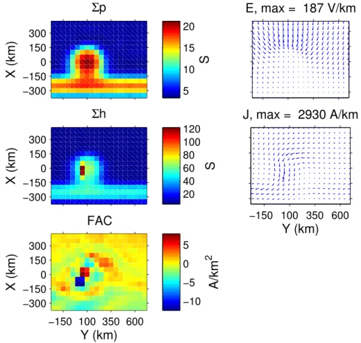
Fig. 2. Model of an omega-band constructed by Amm (1996). Lefthand panels: Pedersen conductance6P, Hall conductance6H and field-aligned current (FAC). Righthand panels: Electric fieldEand horizontal currentJ.
It should be mentioned that in order to simplify these first calculations, we used Cartesian instead of spherical geom-etry, as the model areas are less than 1500 km across. We also neglected the tilt of the magnetic field lines. However, the theory presented in Sect. 3.1 and in the Appendix include also these effects, which are important in a global solution. 4.1 Omega-band
The omega-band model is illustrated in Fig. 2. Lefthand pan-els show the input variables6P,6Hand FAC used in the in-ductive solver. The electric and current fields obtained from the solver should be compared against the model variables shown in the righthand panels of Fig. 2.
The model shown in Fig. 2 is static, an instantaneous snap-shot of the omega-band. We create temporal variations by moving the static model eastward at 2 km s−1, which is a high but still realistic speed (Paschmann et al., 2002, chapter 6).
Figure 3 shows results from the inductive solver. Left-hand panels shows the total electric field (sum of potential and rotational parts) together with associated horizontal and field-aligned currents. FAC is one of the input quantities in the inductive solver, so the result shown in Fig. 3 is
identi-cal to the input model illustrated in Fig. 3, apart from small numerical inaccuracies.
The electric field and current obtained from the inductive solver are in good qualitative agreement with the original model, although their magnitude is too small by almost fac-tor of 2. It is clear that the amount of electrojet type current flowing through the analysis area in East-West direction is severely underestimated, especially in the southern (bottom) side of the model. This behavior is even more evident in the 1-dimensional electrojet model discussed below. As for the electric field, largest errors occur in the low-conductance re-gions around the “”, where errors inJ are magnified in the inverted Ohm’s law.
−300 −150 0 150 300
Edyn, max = 101 V/km
X (km)
Eind, max = 0.8 V/km
−300 −150 0 150 300
Jdyn, max = 1591 A/km
X (km)
Jind, max = 57 A/km
−150 100 350 600 −300
−150 0 150 300
Y (km)
X (km)
FACdyn
A/km
2
−10 −5 0 5
−150 100 350 600 Y (km) FACind
A/km
2
−0.4 −0.2 0 0.2 0.4 0.6 0.8
Fig. 3. Results of the electrodynamic solver for the omega-band model. Lefthand panels: Total electric fieldEdyn, associated horizontal currentsJdynand field aligned currents FACdyn. Righthand panels: Induced part of the total electric fieldEindwith associated currentsJind and FACind.
−300 −150 0 150 300
Eind, max = 1.52 mV/m
X (km)
−150 100 350 600
Y (km)
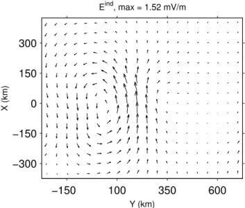
Fig. 4. Induced rotational electric field in the omega-band model calculated with the method of Vanham¨aki et al. (2007).
significant, contributing up to 10% of the total FAC in the tongue.
The results shown in Fig. 3 should be compared against calculations by Vanham¨aki et al. (2007), who used the po-tential part of the electric field as an input variable, instead
of FAC used here. Figure 4 showsEindof the omega-band calculated by Vanham¨aki et al. (2007). The result is very similar, almost identical to the one shown in the upper right panel of Fig. 3, apart from a factor∼2 difference in magni-tudes. Similar magnitude difference is observed also in the WTS model (results not shown). The probable explanation is the different input data: In the present method the total FAC distribution is fixed, so the presence ofEind changes also the potential electric field. Thus the induction effect is distributed by 2 degrees of freedom, the potential and rota-tional parts ofE. In the calculation presented by Vanham¨aki et al. (2007) the potential electric field was fixed, so only the rotationalEwas affected by induction.
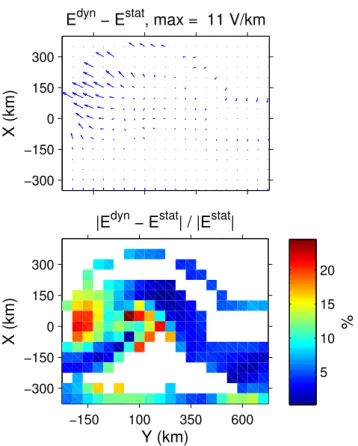
The total induction effect on the electric field is illustrated in Fig. 5. The upper panel shows the difference between the inductive (or electrodynamic) and static solutions,Edyn andEstat, respectively, while the lower panel shows the rel-ative effect. The static solution is obtained by neglecting the time derivative in Eq. (21). As mentioned above, the largest errors in the electric field solution are expected in low-conductance regions. Therefore, only those areas where
|Estat|>5 V km−1and6H>5 S are shown.
−300 −150 0 150 300
E
dyn− E
stat, max = 11 V/km
X (km)
−150 100 350 600
−300 −150 0 150 300
Y (km)
X (km)
|E
dyn− E
stat| / |E
stat|
%
5 10 15 20
Fig. 5.Results for the omega-band model. Upper panel shows the difference between the electric fields obtained from static (Estat) and electrodynamic (Edyn) solvers. Lower panel show the percent-age difference in electric field magnitude. Only those areas where
|Estat|>5 V km−1and6H>5 S are shown.
We made similar calculation also with a WTS model (re-sults not shown) employed by Vanham¨aki et al. (2007). In this case time series was created by moving the model at 10 km s−1 westward, which is again in the upper range of realistic speeds. Here we present only a brief summary of the results.
The Eind in a WTS produced by the inductive solver is very similar in structure to the results obtained earlier by Vanham¨aki et al. (2007). The difference in magnitude is about factor of 2, same as in the omega-band case.
The electric field and horizontal current obtained as out-put from the inductive solver of Sect. 3.1 are in reasonable qualitative agreement with the input model and forJ even the quantitative agreement is fairly good. The electric field is reproduced well in high-conductance areas, but in regions of low conductivity the solution is quite unreliable, probably due to the large contrast between high and low conductance regions (factor of 150 variations in6H, compared to 30 in the omega-band model) and boundary effects caused by the limited model area.
In absolute terms the induction effect is similar to the omega-band, close to 10 V km−1 in many places. The
rel-ative change is 40–60% in many places, although in areas where|E|is small values exceeding 100% are observed. 4.2 1-dimensional electrojet
In addition to the realistic, data-based models described above, we also tested the solver with a simple 1-dimensional electrojet. In this case the 1-D electrojet had a constant elec-tric field and Gaussian conductance profile in the x-direction and no variations in the y-direction. Temporal variations were not included.
This simple test case is worth mentioning because the SECS-based solution algorithm developed in Sect. 3.1 fails almost completely. The main reason for the failure is incor-rect boundary condition. In the SECS-based approach we implicitly assume that divergence and rotation ofE andJ vanish outside the analysis area. In a 1-D electrojet it is pos-sible to add a Cowling channel (Bostr¨om, 1964) to the sys-tem, without affecting the FAC used as input in the inductive solver. The only way to include the Cowling-type part to the solution is to impose explicit boundary conditions. However, this problem affects only regional analysis, as in global scales the solution is unique.
The SECS are intrinsically 2-dimensional, so 1-D struc-tures and open current systems, where large part of the cur-rent flows through the analysis area, are difficult to model with them. This may explain part of the error in the omega-band results. Also this problem is expected to ease in global analysis, where all current systems are, by definition, closed.
5 Discussion and conclusions
The purpose of this article is to present a new inductive (or electrodynamic) ionospheric solver for magnetospheric MHD simulations. We use ionospheric conductances and FAC inferred from the the MHD simulation as the input data, similar to existing electrostatic solvers. In the new solver the internal induction in the ionosphere is taken into account by solving Faraday’ law simultaneously with Ohm’s law and current continuity.
The SECS-based solution algorithm presented in Sect. 3.1 is a modification of the inductive solver presented by Van-ham¨aki et al. (2006) and employed by VanVan-ham¨aki et al. (2007). The main difference is the type of input data used in the solver: Vanham¨aki et al. (2006) assumed that the poten-tial part of the ionospheric electric field is available, whereas here we use the FAC provided by a magnetospheric MHD simulation. Also the local elementary system -based KRM method developed by Vanham¨aki and Amm (2007) is closely related to the solver presented in this article. In fact, as discussed in Sect. 3.3, the theory presented here includes also the KRM solution.
also somewhat similar numerical approach as developed here. Takeda (2008) solved a differential equation for the divergence-free current potentialψ defined in Eq. (7), but presented the curl-free part of the current as a sum of simple vector systems equivalent to the CF SECS used here.
In Sect. 4 we present some preliminary results, that demonstrate the practical applicability of the new induc-tive solver. The results indicate that although the rotational part of the electric field is always local and rather small, about 1 V km−1 at most, it is usually concentrated in areas of high conductivity and therefore drives significant FACs. As the total FAC distribution is fixed, also the potential part of the electric field is indirectly modified by induction. In the omega-band and WTS models (results not shown) the difference in static and electrodynamic solutions may be
∼10 V km−1, or up to 20–40% of the total electric field. Large inductive effects take place in the most dynami-cal ionospheric situations, such as during substorm onsets, which are important in magnetosphere-ionosphere coupling. We may expect that the difference between simulation runs using electrostatic and electrodynamic ionospheric solvers solutions increases with time, as the slightly different iono-spheric solution affect the temporal evolution of the MHD simulation.
As discussed in Sect. 4, the output of the new solver is usually in good qualitative agreement with the correct E andJ of the input model, but some errors are also present. Largest errors inJare probably related to the boundary con-ditions needed in regional analysis, so results of global anal-ysis should be more reliable.
The electric field produced by the inductive solver includes a rotational part, which can’t be mapped to the magneto-sphere as simply as a potential field, as discussed in Sect. 3.2. One way to overcome the mapping problem would be to describe the magnetosphere-ionosphere coupling in terms of Alfv´en wave propagation and reflection, like the model proposed by Lysak and Song (2006) discussed in Sect. 2.3. However, an Alfv´enic model would be more complicated to couple to an MHD simulation than the inductive solver pre-sented here, although recently Yoshikawa et al. (2010) have presented a possible coupling scheme.
The results presented in Sect. 4 indicate that the rotational part itself is rather small, but inductive change of the poten-tial field is much larger. If this is true also in a global solution, and is not related to the problem of boundary conditions in regional analysis, then it may be feasible to simply ignore the rotational part of the electric field and map only the potential part to the MHD simulation.
In the present theoretical study we settled for present-ing the theoretical basis of the new ionospheric solver and demonstrating its usability. Actual coupling of the new in-ductive solver to an magnetospheric MHD simulation is a topic for future studies.
Appendix A
In this Appendix we describe how to form the matricesM1,2, L1,2 andN1,2 defined in Eqs. (12), (17) and (20), respec-tively.
A1 Matrices M1,2
According to Eqs. (12)–(15) componentM1(2v−1,u)of the ma-trixM1gives that part ofJθ at locationrvthat is contributed by a CF SECS located atrelu. Similarly, componentM1(2v,u) gives curl-free part ofJφatrv. Geometry of the situation is illustrated in Fig. A1. The vector field of each individual CF SECS is given in Eq. (10), where the scaling factorVcf cor-responds to the components of vectordivJ. The remaining task is to convert the angleθ′and unit vectoreˆφ′ defined in a SECS-centered coordinate system to the geographical sys-tem.
It is a straightforward exercise in spherical geometry to show that
M1(2v−1,u)= Au 4π RI
cosθuel−cosθvcosθ′ sinθv(1−cosθ′)
, (A1)
M1(2v,u)= − Au 4π RI
sinθuelsin(φelu−φv)
1−cosθ′ , (A2)
whereAuis the area of the grid cell centered atrelu and cosθ′=cosθvcosθuel+sinθvsinθuelcos(φ
el
u−φv). (A3) Components of the matrixM2are obtained in a similar fash-ion from the DF SECS defined in Eq. (10). The result is simply
M2(2v−1,u)= −M1(2v,u), (A4) M2(2v,u)=M1(2v−1,u). (A5) A2 Matrices L1,2
MatricesL1,2are defined in Eq. (17). ComponentL(v,u)1 of the matrixL1gives curl of the electric field at pointrvcaused by the CF SECS atrelu, while matrixL2is associated with the divergence-free elementary systems. It is straightforward to evaluate the curl of Eq. (16),
(∇ ×E)r = −∇Rθ φ·J−Rθ φ∇ ·J+(∇Rφφ×J)r+
+Rφφ(∇ ×J)r− 1 RIsinθ
∂ (R−Jθ)
∂ φ , (A6)
where components of the resistance tensor defined in Eq. (16) are abbreviated as
R=
Rθ θ Rθ φ
−Rθ φRφφ
(θ,φ)
θ
θ
θ
(θ ,φ )
φ − φ
el el
el
C
A
’
Pole
el
Fig. A1. Geometry of calculating components of matrices M1,2. The elementary system is located at(θel,φel)and the vector field is evaluated at(θ,φ).θ′is the latitude of the point(θ,φ)in the coordinate system centered at the elementary system.
Fig. A2.Curl-free elementary system with tilted FAC at the pole. After Fukushima (1976).
and the difference of the diagonal components is R−=Rθ θ−Rφφ=
1 60−
6P 6P2+6H2
!
cosI. (A8)
The divergence and curl of the DF and CF elementary sys-tems defined in Eqs. (10), (11) are
∇ ·Jel,cf=(∇ ×Jel,df)r=I0 δ2(rel−r)− 1 4π R2I
! , (A9)
(∇ ×Jel,cf)r= ∇ ·Jel,df=0. (A10) Components ofL1,2matrices can be deduced from Eqs. (12), (17), (A6) and (A9)–(A10) as
L1(v,u)= −M1(2v−1,u)(Rθ φ;θ+Rφφ;φ)−M1(2v,u)(Rθ φ;φ−Rφφ;θ)
−∂ (R−M
(2v−1,u)
1 )
RIsinθv∂ φ −
Rθ φ δu,v−
Au
4π R2I !
, (A11)
L2(v,u)= −M2(2v−1,u)(Rθ φ;θ+Rφφ;φ)−M2(2v,u)(Rθ φ;φ−Rφφ;θ)
−∂ (R−M
(2v−1,u)
2 )
RIsinθv∂ φ +
Rφφ δu,v−
Au
4π RI2 !
. (A12) In the above formulas gradients are denoted as
Rθ φ;θ:= 1 RI
∂ Rθ φ
∂ θ , (A13)
and so on. Functionδu,vis defined so that
δu,v=
1 ifrv∈cell u
0 otherwise , (A14)
andAuis the area of the grid cell centered atrelu. A3 Matrices N1,2
associated with the DF SECS. When calculating the mag-netic field of a CF SECS, the FAC associated with the diver-gence of the horizontal current has to be included. Accord-ing to Eq. (A9), there is a delta-function FAC at the pole of the system and uniform, oppositely directed FAC elsewhere. We model the polar FAC as a tilted semi-infinite line current, while the uniform FAC is assumed to flow radially. The ge-ometry of the uniform FAC need not be realistic, because we expect that in global scales the inward and outward flowing line currents will balance each other, and consequently the uniform FACs of the CF SECS will sum to zero.
Figure A2 illustrates the FAC distribution of a curl-free SECS and the way it can be decomposed into a purely ra-dial FAC system plus a line current wedge. According to Fukushima’s theorem the radial magnetic field of current sys-tem illustrated in the middle panel is zero (Fukushima, 1976). It is easy to show that the vertical line current of the current wedge also hasBr=0. The remaining task is to calculate the radial magnetic field of the tilted semi-infinite line current.
Let us orient the primed, SECS centered coordinate system so that the line current flows along the zero meridian. The point(θv,φv)where we want to calculateBris(θ′,φ′)in the primed system (see Fig. A1). cosθ′is given in Eq. (A3) and
φ′=A+D+180◦, (A15)
whereDis the declination angle of the magnetic field (posi-tive eastward). According to spherical trigonometry
sinA=sinθvsin(φ el u−φv)
sinθ′ , (A16)
cosA=cosθv−cosθ ′cosθel
u
sinθ′sinθuel . (A17)
The Biot-Savart law givesBras
Br= µ0Iel,cf
4π Z
line
(dl×V)r
|V|3 , (A18)
whereIel,cf is the scaling factor of the CF SECS,dl is di-rected along the line current and V is a vector from r′= (RI,θ′,φ′)todl. It is straightforward (although somewhat tedious) to expressdlandV in terms of the primed unit vec-tors at pointr′ and evaluate the integral. In any case, the elements of the matrixN1are
N1(v,u)= −µ0Au 4π RI
sinθ′sinφ′cosI α−β2
1+√β
α
, (A19)
whereI is the inclination of the magnetic field,Auis the area of the grid cell centered atrel
u and
α=2−2cosθ′, (A20)
β=sinθ′cosφ′cosI+(1−cosθ′)sinI. (A21)
Magnetic field of a DF SECS was calculated by Amm and Viljanen (1999). Components of the matrixN2are obtained from the expression of the radial magnetic field,
N2(v,u)=µ0Au 4π RI
1
√
2−2cosθ′−1
. (A22)
Acknowledgements. The work of H. Vanham¨aki is supported by the Academy of Finland (project number 126552). The author wishes to thank O. Amm, R. Fujii, A. Yoshikawa and A. Ieda for useful discussions and comments on the manuscript.
Topical Editor M. Pinnock thanks C. L. Waters and S. C. Buchert for their help in evaluating this paper.
References
Amm, O.: Improved electrodynamic modeling of an omega band and analysis of its current system, J. Geophys. Res., 101, 2677– 2683, 1996.
Amm, O.: Ionospheric elementary current systems in spherical co-ordinates and their application, J. Geomagnetism and Geoelec-tricity, 49, 947–955, 1997.
Amm, O. and Viljanen, A.: Ionospheric disturbance magnetic field continuation from the ground to the ionosphere using spherical elementary current systems, Earth, Planets and Space, 51, 431– 440, 1999.
Bostr¨om, R.: A model of the auroral electrojets, J. Geophys. Res., 69, 4983–4999, 1964.
Brekke, A.: Physics of the upper polar atmosphere, John Wiley & Sons, ISBN 0-471-96018-7, 1997.
Buchert, S.: Magneto-optical Kerr effect for a dissipative plasma, J. Plasma Phys., 59, 39–55, 1998.
Fukushima, N.: Generalized theorem for no ground magnetic ef-fect of vertical currents connected with Pedersen currents in the uniform-conductivity ionosphere, Rep. Ionos. Space. Res. Japan, 30, 35–40, 1976.
Glassmeier, K.-H.: On the influence of ionospheres with non-uniform conductivity distribution on hydromagnetic waves, J. Geophys., 54, 125–137, 1984.
Janhunen, P.: GUMICS-3 – A global ionosphere-magnetosphere coupling simulation with high ionospheric resolution, ESA Sym-posium Proceedings on Environmental Modelling for Space-based applications, ESTEC, Noordwijk, NL, 18–20 September 1996, ESA SP-392, 1996.
Janhunen, P.: On the possibility of using an electromagnetic iono-sphere in global MHD simulations, Ann. Geophys., 16, 397–402, doi:10.1007/s00585-998-0397-y, 1998.
Kamide, Y., Richmond, A. D., and Matsushita, S.: Estimation of ionospheric electric fields, ionospheric currents, and field-aligned currents from ground magnetic records, J. Geophys. Res., 86, 801–813, 1981.
Lyon, J. G., Fedder, J. A., and Mobarry, C. M.: The Lyon-Fedder-Mobarry (LFM) global MHD magnetospheric simulation code, J. Atmos. Solar-Terr. Phys., 66, 1333–1350, 2004.
Lysak, R. and Song, Y.: A three-dimensional model of the prop-agation of Alfv´en waves through the auroral ionosphere: First results, Adv. Space Res., 28, 813–822, 2001.
Paschmann, G., Haaland, S., and Treumann, R. (Eds.): Auroral Plasma Physics, Space Sci. Rev., 103, 1–486, 2002.
Raeder, J., Berchem, J., and Ashour-Abdalla, M.: The geospace environment grand challenge: Results from a global geospace circulation model, J. Geophys. Res., 103, 14787–14797, 1998. Sciffer, M. D., Waters, C. L., and Menk, F. W.: Propagation of ULF
waves through the ionosphere: Inductive effect for oblique mag-netic fields, Ann. Geophys., 22, 1155–1169, doi:10.5194/angeo-22-1155-2004, 2004.
Takeda, M.: Effects of the induction electric field on iono-spheric current systems driven by field-aligned currents of magnetospheric origin, J. Geophys. Res., 113, A01306, doi:10.1029/2007JA012662, 2008.
Tanaka, T.: The state transition model of the substorm onset, J. Geo-phys. Res., 105, 21081–21096, 2000.
Untiedt, J. and Baumjohann, W.: Studies of polar current systems using the IMS Scandinavian magnetometer array, Space Sci. Rev., 63, 245–390, 1993.
Vanham¨aki, H. and Amm, O.: A new method to estimate iono-spheric electric fields and currents using data from a local ground magnetometer network, Ann. Geophys., 25, 1141–1156, doi:10.5194/angeo-25-1141-2007, 2007.
Vanham¨aki, H., Amm, O., and Viljanen, A.: New method for solving inductive electric fields in the non-uniformly conducting ionosphere, Ann. Geophys., 24, 2573–2582, doi:10.5194/angeo-24-2573-2006, 2006.
Vanham¨aki, H., Amm, O., and Viljanen, A.: Role of inductive elec-tric fields and currents in dynamical ionospheric situations, Ann. Geophys., 25, 437–455, doi:10.5194/angeo-25-437-2007, 2007. Waters, C. L. and Sciffer, M. D.: Field line resonant frequencies and
ionospheric conductance: Results from a 2-D MHD model, J. Geophys. Res., 113, A05219, doi:10.1029/2007JA012822, 2008. Yoshikawa, A. and Itonaga, M.: Reflection of shear Alfv´en waves at the ionosphere and the divergent Hall current, Geophys. Res. Lett., 23, 101–104, 1996.