On: 06 January 2012, At : 04: 33 Publisher: Taylor & Francis
I nform a Lt d Regist ered in England and Wales Regist ered Num ber: 1072954 Regist ered office: Mort im er House, 37- 41 Mort im er St reet , London W1T 3JH, UK
Optimization
Publicat ion det ails, including inst ruct ions f or aut hors and subscript ion inf ormat ion:
ht t p: / / www. t andf online. com/ loi/ gopt 20
Interior point filter method for
semi-infinite programming problems
Ana I. Pereira a , M. Fernanda P. Cost a b & Edit e M. G. P. Fernandes c
a
Depart ment of Mat hemat ics – ESTiG, Polyt echnic Inst it ut e of Bragança, 5301-857 Bragança, Port ugal
b
Depart ment of Mat hemat ics and Applicat ions, Universit y of Minho, 4800-058 Guimarães, Port ugal
c
Algorit mi R&D Cent er, Universit y of Minho, 4710-057 Braga, Port ugal
Available online: 04 Oct 2011
To cite this article: Ana I. Pereira, M. Fernanda P. Cost a & Edit e M. G. P. Fernandes (2011): Int erior point f ilt er met hod f or semi-inf init e programming problems, Opt imizat ion, 60: 10-11, 1309-1338 To link to this article: ht t p: / / dx. doi. org/ 10. 1080/ 02331934. 2011. 616894
PLEASE SCROLL DOWN FOR ARTI CLE
Full t erm s and condit ions of use: ht t p: / / w w w.t andfonline.com / page/ t erm s- and-condit ions
This art icle m ay be used for research, t eaching, and privat e st udy purposes. Any subst ant ial or syst em at ic reproduct ion, redist ribut ion, reselling, loan, sub- licensing, syst em at ic supply, or dist ribut ion in any form t o anyone is expressly forbidden.
The publisher does not give any warrant y express or im plied or m ake any represent at ion t hat t he cont ent s w ill be com plet e or accurat e or up t o dat e. The accuracy of any
Vol. 60, Nos. 10–11, October–November 2011, 1309–1338
Interior point filter method for semi-infinite programming problems
Ana I. Pereiraa*, M. Fernanda P. Costab
and Edite M.G.P. Fernandesc
a
Department of Mathematics – ESTiG, Polytechnic Institute of Braganc¸a, 5301-857 Braganc¸a, Portugal;bDepartment of Mathematics and Applications, University of Minho,
4800-058 Guimara˜es, Portugal;cAlgoritmi R&D Center, University of Minho, 4710-057 Braga, Portugal
(Received 31 August 2009; final version received 17 August 2011)
Semi-infinite programming (SIP) problems can be efficiently solved by reduction-type methods. Here, we present a new reduction method for SIP, where the multi-local optimization is carried out with a stretched simulated annealing algorithm, the reduced (finite) problem is approximately solved by a Newton’s primal–dual interior point method that uses a novel two-dimensional filter line search strategy to guarantee the convergence to a KKT point that is a minimizer, and the global convergence of the overall reduction method is promoted through the implementation of a classical two-dimensional filter line search. Numerical experiments with a set of well-known problems are shown.
Keywords: nonlinear optimization; semi-infinite programming; interior point; filter method; line search
AMS Subject Classifications: 90C30; 90C34; 90C51
1. Introduction
A reduction-type method based on a primal–dual interior point filter method for nonlinear semi-infinite programming (SIP) is proposed. To allow convergence from poor starting points, a backtracking line search filter strategy is implemented. The SIP problem is considered to be of the form
minfðxÞsubject togðx,tÞ 0, for everyt2T, ðPÞ
whereTRmis a nonempty set defined by T¼{t2Rm:v(t)0}. Here, we assume that the setTdoes not depend onx. If the setTdepends onx, the problem is called as generalized semi-infinite programming problem [31,32,38].
The nonlinear functions f:Rn!R and g:RnT!R are twice continuously differentiable with respect to x, and g is continuously differentiable function with respect tot.
There are many problems in the engineering area that can be formulated as SIP problems. Approximation theory [15], optimal control [10], mechanical stress of
*Corresponding author. Email: [email protected]
ISSN 0233–1934 print/ISSN 1029–4945 online ß2011 Taylor & Francis
http://dx.doi.org/10.1080/02331934.2011.616894 http://www.tandfonline.com
materials and computer-aided design [43], air pollution control [37], robot trajectory planning [36], financial mathematics and computational biology and medicine [42] are some examples. For a review of other applications, the reader is referred to [7,15,25,28,38].
The numerical methods that are mostly used to solve SIP problems generate a sequence of finite problems. There are three main ways of generating the sequence: by discretization, exchange and reduction methods [10,25,36]. Methods that solve the SIP problem on the basis of the KKT system derived from the problem are emerging in the literature [12–14,23,24,29,30,43].
This work aims to describe a reduction method for SIP. Conceptually, the method is based on the local reduction theory. The focus of our proposal is on an interior point filter line search-based method, to compute an approximation to the finite optimization problem that emerges in a global reduction algorithm context, for solving a nonlinear SIP problem. The global convergence analysis of the interior point filter algorithm to a KKT point that is a minimizer is also included. This work comes in the sequence of a previous penalty-based reduction-type method presented in [21]. We have been observing that, when solving SIP problems with this type of methods, the performance depends strongly on the user-defined penalty parameters that are present in penalty functions when solving the reduced finite problem, and in merit functions when promoting the overall algorithm global convergence.
Here, we aim to simplify the solution method while solving the reduced problem, as well as to improve efficiency in terms of number of iterations required by the overall algorithm. In the new algorithm, the multi-local procedure uses the stretched simulated annealing method [21]. To solve the reduced finite optimization problem, we propose a Newton’s primal–dual interior point method that uses a novel two-dimensional filter line search to guarantee the convergence to a KKT point, that is a minimizer. It is shown that every limit point of the sequence of iterates generated by the algorithm is feasible and satisfies the complementarity condition. We also show that there exists at least a limit point that is a KKT point of the problem. Finally, to promote convergence from any initial approximation, a two-dimensional filter methodology, as proposed in [6], is also incorporated into the reduction algorithm. This article is organized as follows. In Section 2, we present the basic ideas behind the local reduction to finite problems. Section 3 is briefly devoted to the multi-local procedure and Section 4 contains a detailed description of the herein proposed primal–dual interior point filter line search method for solving the reduced optimization problem. The global convergence analysis of the algorithm is also included. Section 5 presents the filter methodology to promote global convergence of the reduction algorithm and Section 6 lists the conditions for its termination. Finally, Section 7 contains some numerical results and conclusions.
2. First-order optimality conditions and reduction method
In this section we present some definitions and the optimality conditions of problem (P). We denote thefeasible setof problem (P) byX, where
X¼x2Rn:gðx,tÞ 0, for everyt2T:
A feasible point x2X is called a strict local minimizer of problem (P) if there
exists a positive valuesuch that
8x2X:fðxÞ fðxÞ40^kxxk5^x6¼x,
where kk represents the euclidean norm. Forx2X, theactive index set, T0ðxÞ, is
defined by
T0ðxÞ ¼t2T:gðx,tÞ ¼0:
We first assume the following.
ASSUMPTION 2.1 Let x2X.The linear independence constraint qualification(LICQ) holds atx,i.e.rxgðx,tÞ,t2T0ðxÞis a linearly independent set.
Since LICQ implies theMangasarian–Fromovitz constraint qualification(MFCQ) [15], we can conclude that forx2Xthere exists a vectord2Rn
such that for every
t2T0ðxÞ the condition rxgðx,tÞTd50 is satisfied. A direction d that satisfies this
condition is called astrictly feasible direction. Further, the vectord2Rnis astrictly feasible descent directionif the following conditions hold:
rfðxÞTd50, rxgðx,tÞTd50, for everyt2T0ðxÞ: ð1Þ
Ifx2X is a local minimizer of the problem (P) then there will not exist a strictly
feasible descent directiond2Rn\ {0n}, where 0nrepresents the null vector ofRn.
THEOREM2.2 [15] Letx2X.Suppose that there is no direction d2Rn\ {0n}satisfying
rfðxÞTd0 and rxgðx,tÞTd0, for every t2T0ðxÞ:
Thenx is a strict local minimizer of SIP .
Since Assumption 2.1 is verified, the set T0ðxÞ is finite. Suppose that T0ðxÞ ¼t1,. . .,tp, then pn. If x is a local minimizer of problem (P) and if the
MFCQ holds atx, then there exist nonnegative valueslforl¼1,. . .,psuch that
rfðxÞ þX p
l¼1
lrxgðx,tlÞ ¼0n: ð2Þ
This is the Karush–Kuhn–Tucker (KKT) condition of problem (P).
Many papers exist in the literature devoted to the reduction theory [1,2,9,10,22,25,33]. The main idea is to describe, locally, the feasible set of the problem (P) by a finite set of constraints. Assume thatxis a feasible point and that
eachtl2TTðxÞis a local maximizer of the so-calledlower level problem
max
t2T gð
x,tÞ, ð3Þ
satisfying the following condition:
gðx,tlÞ g
ML, l¼1,. . .,L, ð4Þ
whereL pand represents the cardinality ofT,MLis a positive constant andgis the global solution value of (3).
ASSUMPTION 2.3 For any fixedx2X,each tl2T is an strict local maximizer ,i.e. 940, 8t2T:gðx,tlÞ4gðx,tÞ ^kttlk5^t6¼tl:
When the setTis compact,xis a feasible point and Assumption 2.3 holds, there
exists a finite number of local maximizers of the problem (3) and the implicit function theorem can be applied, under some constraint qualifications [15]. So, it is possible to conclude that there exist open neighbourhoodsU, ofx, andVl, oftl, and
implicit functionst1ðxÞ,. . .,tLðxÞdefined as (i) tl:U!Vl\T, forl¼1,. . .,L;
(ii) tlðxÞ ¼tl, forl¼1,. . .,L;
(iii) 8x2U, tl(x) is a non-degenerate and strict local maximizer of the
problem (3); so that
fx2U :gðx,tÞ 0, for everyt2Tg , fx2U:gðx,tlðxÞÞ 0,l¼1,. . .,Lg:
So it is possible to replace the infinite set of constraints by a finite set that is locally sufficient to define the feasible region. Thus the problem (P) is locally equivalent to the so-calledreduced(finite)optimization problem
min
x2U
fðxÞ subject toglðxÞ gðx,tlðxÞÞ 0, l¼1,. . .,L ð5Þ
whereU is an open neighbourhood ofxandtl(x),l¼1,. . .,L, are implicitly defined
functions satisfying (ii) and (iii) above.
A reduction method then emerges when any method for finite programming
is applied to solve the locally reduced problem (5). Conceptually, the
reduction method resumes to an iterative process. Thus, at each iteration, indexed by k, the Algorithm 2.1 shows the main procedures of the proposed reduction method.
Algorithm 2.1(Global reduction algorithm)
Fork¼1, 2,. . .an approximationxkto the SIP problem is required:
(1) Based onxk, compute the set Tk, solving problem (3), with condition (4). (2) Based on the set Tk, implement at most imax iterations to get an
approximationxk,i, by solving the reduced problem (5).
(3) Use a globalization technique to compute a new approximation xkþ1 that improves significantly overxk.
(4) Use termination criteria to decide if the iterative process should terminate.
The remaining part of this article presents our proposals for the four steps of the global reduction algorithm, Algorithm 2.1, for SIP. An algorithm to compute the set
Tkis known in the literature as a multi-local procedure. In this article, a stretched simulated annealing algorithm that has been previously applied in other reduction-type methods is used (see [18–21] for details). To solve the reduced problem (5), a Newton’s primal–dual interior point method is proposed. Further, a filter line search technique is incorporated into the interior point algorithm in order to promote global convergence, whatever may be the initial approximation. Each entry
in the filter is composed by two components that measure the KKT error. As explained later in this article, the components come naturally from the KKT conditions for the reduced problem (5). The first component measures feasibility and complementarity, and the second measures optimality. Additionally to enforce progress towards a minimizer, and whenever a descent direction for the logarithmic barrier function (from the barrier problem associated with the reduced problem to be solved) is computed, a sufficient reduction is also imposed on that function by means of an Armijo condition. This is the main contribution of this article. As far as we know, a primal–dual interior point filter line search technique has not been applied in a nonlinear SIP context. Furthermore, the proposed two-dimensional filter line search strategy is a novelty in the field of interior point methods. The global convergence analysis of the interior point algorithm is also included. Finally, convergence of the overall reduction method to an SIP solution is encouraged by implementing a filter line search technique. The filter here aims to measure sufficient progress by using the constraint violation and the objective function value. This filter strategy has been shown to behave well for SIP problems when compared with merit function approaches [18,19].
3. The multi-local procedure
The multi-local procedure is used to compute the setTk, i.e. the local solutions of the problem (3) that satisfy (4). Some procedures to find the local maximizers of the constraint function consist of two phases: first, a discretization of the setTis made and all maximizers are evaluated on that finite set; second, a local method is applied in order to increase the accuracy of the approximations found in the first phase (e.g. [2]). Our proposal combines the function stretching technique, proposed in [17], with a simulated annealing (SA)-type algorithm – the ASA variant of the SA in [11]. This is a stochastic point-to-point global search method that generates the elements ofTksequentially.
The function stretching technique was initially proposed in [17], in a particle swarm optimization algorithm context, to provide a way to escape from a local solution, driving the search to a global one. When a local (non-global) solution,bt, is detected, this technique reduces by a certain amount the objective function values at all pointstthat verifygðtÞ gðbtÞ, and maintains the function values for all
t such that gðtÞ4gðbtÞ. The process is repeated until the global solution is encountered.
Since we need to compute global as well as local solutions, the inclusion of the function stretching technique aims to prevent the convergence of the ASA algorithm to an already detected solution. Let t1be the first computed global solution. The function stretching technique is applied, only locally, in order to transformg(t) in a neighbourhood oft1, sayV"1ðt1Þ("1>0), decreasing the function values on the region
V"1ðt1Þ, leaving all the other maxima unchanged. That particular maximum, g(t1),
disappears although all the other maxima are left unchanged. The ASA algorithm is then applied to the modified objective function to detect a global solution of the new problem. This iterative process terminates if no other solution is found for a set of
KMLconsecutive iterations (see [18,21] for details).
4. Finite optimization procedure
The sequential quadratic programming method is the mostly used finite programming procedure in reduction-type methods for solving SIP problems. Usually, they use the
L1and L1 merit functions and rely on a trust region framework to ensure global
convergence (see, e.g. [2,22,33]). Penalty methods with exponential and hyperbolic penalty functions have already been tested with some success [19,21]. However, to solve finite inequality constrained optimization problems, Newton’s primal–dual interior point methods [5,26,27,34,35] and primal–dual barrier methods [5,39–41] have shown to be competitive and even more robust than sequential quadratic program-ming and penalty-type methods. This is the motivation of this work. Incorporating a primal–dual interior point method into a reduction-type method for nonlinear SIP is the main goal to improve the efficiency over previous reduction methods. The global convergence analysis of the proposed algorithm is also included.
For simplicity, we now consider the special case of SIP problems where
T¼{t2Rm:atb}. To solve the reduced (finite) problem (5), we propose the use of an infeasible primal–dual interior point (P-DIP) method. We remark that this infeasible version of the method corresponds to the reformulation of the reduced problem (5) into an equivalent problem, where the unique inequality constraints are simple nonnegativity constraints. So, in this methodology, the first step is to introduce slack variables to replace all inequality constraints by equality constraints and simple nonnegativity constraints. Hence, adding nonnegative slack variables
w¼ ðw0,w1,. . .,w
Lkþ1ÞTto the inequality constraints, the problem (5) is rewritten as follows:
min
x2UkRn
,w2RLkþ2
fðxÞsubject toglðxÞ þwl¼0, l¼0,. . .,Lkþ1 ,wl 0, ð6Þ
whereg0(x)¼g(x,a) andgLkþ1ðxÞ ¼gðx,bÞcorrespond to the values of the constraint function g(x,t) at the lower and upper limits of set T. The KKT conditions for problem (6) are
rxLðx,w,z,yÞ ¼ rfðxÞ þ rgðxÞz¼0
rwLðx,w,z,yÞ ¼zy¼0 rzLðx,w,z,yÞ ¼gðxÞ þw¼0
wTy¼0
w 0, y 0,
ð7Þ
where L(x,w,z,y)¼f(x)þ(g(x)þw)TzwTy is the Lagrangian function of the problem (6) and z and y are the Lagrange multiplier vectors associated with constraints g(x)þw¼0 and w 0, respectively. From the second equation in (7),
z¼y, meaning that, at the solution, the multipliers associated with the equality constraints g(x)þw¼0 are the same as the multipliers associated with the constraintsw 0, and replacing yields
Fðx,w,yÞ
rfðxÞ þ rgðxÞy¼0
gðxÞ þw¼0
WYe¼0
8 > < > :
w 0, y 0,
ð8Þ
where W¼diagðw0,. . .,wLkþ1Þ and Y¼diagðy0,. . .,yLkþ1Þ are diagonal matrices ande2RLkþ2 is a vector of ones.
In this method, the term ‘infeasible’ refers to the fact that dual and primal feasibilities (first and second equations in (8)) are not required at the beginning although they are enforced throughout the iterative process. The term ‘primal–dual’ refers to the fact that the Lagrange multipliersyare treated as independent variables in all calculations, as we do with the primal variablesx and w. The term ‘interior point’ is used since the slack variables,w, and the dual variables,y, are required to satisfy the bounds in (8) strictly at the beginning and throughout the iterative process. By satisfying these bounds, the method avoids spurious solutions, i.e. points that satisfy the first three equations in (8) but notw 0 andy 0.
When Newton’s method is applied to the system (8) to get the search directions Dx,DwandDy, it deals with the linearized complementarity equation
YDwþWDy¼ WYe
that may cause a serious problem. This equation forces the iterate to stick to the boundary of the feasible region once it approaches that boundary. This means that if the componentl of the current iterate, wi
l, becomes zero and yil40, it will remain
zero in all iterations afteri. The same is true for the components of the vectoryi. This drawback is solved by modifying the Newton formulation so that zero variables become nonzero in subsequent iterations. This is done replacing the complementarity equationWYe¼0 by the perturbed complementarity WYe¼be, whereb40. The following perturbed KKT conditions then appear:
F^ðx,w,yÞ
rfðxÞ þ rgðxÞy¼0
WYebe¼0
gðxÞ þw¼0
8 > < > :
w 0, y 0:
ð9Þ
We note that the perturbed KKT conditions for problem (6), given by (9), are equivalent to the KKT conditions of the barrier problem associated with problem (6), in the sense that they have the same solutions,
min
x2UkRn,w2RLkþ2
’^ðx,wÞ fðxÞ b
X Lkþ1
l¼0
lnðwlÞ
subject to gðxÞ þw¼0,
ð10Þ
where’^ðx,wÞis the logarithmic barrier function, for a fixedb40 [5].
Applying Newton’s method to the systemF^ðx,w,yÞ ¼0 in (9), we obtain a linear system to compute the search directionsDx,Dw,Dy
Hðx,yÞ 0 rgðxÞ
0 Y W
rgðxÞT I 0
2 6 4
3 7 5
Dx
Dw
Dy 2 6 4
3 7
5¼
rfðxÞ þ rgðxÞy WYebe
gðxÞ þw 2
6 4
3 7
5, ð11Þ
where Hðx,yÞ ¼ r2f xð Þ þPLkþ1
l¼0 ylr2glðxÞ is the Hessian of the Lagrangian. This
system is not symmetric, but is easily symmetrized by multiplying the second
equation byW1, yielding
Hðx,yÞ 0 rgðxÞ
0 W1Y I
rgðxÞT I 0
2 6 4
3 7 5
Dx
Dw
Dy 2 6 4
3 7
5¼
W1
^
2 6 4
3 7
5, ð12Þ
where we define
ðx,yÞ ¼ rfðxÞ þ rgðxÞy, ^ ^ðw,yÞ ¼WYebe
ðx,wÞ ¼gðxÞ þw: ð13Þ
Let N(x,w,y)¼H(x,y)þ rg(x)W1Yrg(x)T denote the dual normal matrix. THEOREM 4.1 If N is nonsingular,then (12)has a unique solution.In particular,
Dx¼ N1rfðxÞ bN1rgðxÞW1eN1rgðxÞW1Y
Dw¼ rgðxÞTN1rfðxÞ þbrgðxÞTN1rgðxÞW1e
I rgðxÞTN1rgðxÞW1Y:
The proof of these results is left for the Appendix of this article.
It is known that if the initial approximation is close enough to the solution, methods based on the Newton’s iteration converge quadratically under appropriate assumptions. For poor initial points, a backtracking line search can be implemented to promote convergence to the solution of problem (6) [16]. After the search directions have been computed, the idea is to choose i2 ð0, i
max, at iteration i,
so thatxk,iþ1¼xk,iþ iDxi,wk,iþ1¼wk,iþ iDwiandyk,iþ1¼yk,iþ iDyiimprove over a primal–dual estimate solution (xk,i,wk,i,yk,i) for problem (6). The indexirepresents the iteration counter of this inner cycle. The parameter i
max represents the longest
step size that can be taken along the direction to maintainwiandyistrictly positive. Thus the maximal step size i
max2 ð0, 1is defined by i
max¼maxf 2 ð0, 1:w
iþ Dwi ð1Þwi, yiþ Dyi ð1Þyig ð14Þ
for a fixed parameter2(0, 1) (close to one).
The strategy to recover b at each iteration considers a fraction of the average complementarity
b
¼c, with¼
wTy
Lkþ2, ð15Þ
wherec2(0, 1) is a centring parameter. This choice ofballows a dynamic reduction
of(see inequality (23) in Lemma 4.10).
To measure the progress, a penalty or merit function could be used. Although most penalty or merit functions are defined as a linear combination of the objective function and a measure of the constraint violation, there are others that also depend on the Lagrange multiplier vectors, and there is a particular choice that is defined as the squared l2-norm of the residual vectorF(x,w,y) [5]. In the latter, the algorithm may be more likely to converge to stationary points that are not local minimizers. In general, penalty or merit functions depend on a penalty parameter. Unfortunately, a suitable value for the penalty parameter depends on the optimal
solution of the problem. Thus, the choice of the penalty parameter is a difficult issue. On the other hand, Fletcher and Leyffer [6] proposed a filter method as an alternative to a merit function to guarantee global convergence in algorithms for nonlinear optimization. This technique incorporates the concept of nondominance to build a filter that is able to accept iterates if they improve either the objective function or the constraint violation, instead of a linear combination of those two measures. So the filter replaces the use of merit functions, avoiding the update of penalty parameters. The filter technique has already been adapted to interior point methods [3,4,27,34,39–41]. Different filters with two- and three-dimensional entries have been proposed in this context.
4.1. A novel two-dimensional filter line search approach
The herein proposed two-dimensional filter line search strategy aims to reduce the residual vector F(x,w,y) and to enforce progress towards a KKT point that is a minimizer. According to the KKT conditions (8), each entry in the filter is herein defined by
ðx,w,yÞ ¼k k 2þ 0 2 and oðx,yÞ ¼k k 22: ð16Þ
The first entry in the filter,(x,w,y), aims to measure feasibility and complemen-tarity of each trial iterate, while the other,o(x,y), measures optimality. Recall that
0WYe, according to a previous definition (13). Convergence to KKT points that are minimizers will be guaranteed when sufficient reductions onoas well as on the
logarithmic barrier function,’^, are also imposed, as shown later on in this section. Borrowing the ideas presented in [39–41], our filter is defined as a set Fi that
contains values ofandothat are prohibited for a successful iterate in iteration i.
At the beginning of the iterative process, the filter is initialized to
F0 ð,oÞ 2R2: max40,o omax40
:
After computing the search directions Di¼(Dxi,Dwi,Dyi) by (12), a new iterate
uk,iþ1¼uk,iþ iDi, whereu¼(x,w,y), might be acceptable if the following condition, known as ‘acceptance condition’, holds:
iþ1ð11Þi or ioþ1
i
o2i, ðAC-rÞ
where1,22(0, 1). For simplicity, the following notation is usediþ1¼(uk,iþ1) and
oiþ1¼oðxk,iþ1,yk,iþ1Þ. To prevent the convergence to a point that is feasible and
satisfies the complementarity condition but is nonoptimal, another set of conditions must be satisfied for a trial pointuk,iþ1to be acceptable. Ifimin(formin>0) and the ‘switching conditions’
mi
1ð Þ50, mi2ð Þ50 and mi
1ð Þ4 i r
and mi
2ð Þ4 i
r ðSC-rÞ
hold, where
mi1ð Þ ¼ ir’
^
ðxi,wiÞTD1,i, withD1,i¼ ðDxi,DwiÞ, mi2ð Þ ¼ ir
oðxi,yiÞTD2,i, withD2,i¼ ðDxi,DyiÞ
ð17Þ
and ’^ðx,wÞ is the barrier function (10), then uk,iþ1 is acceptable if sufficient reductions on’^ ando, according to the ‘Armijo condition’,
’i^þ1’
i
^
þmi1ð Þ and ioþ1ioþmi2ð Þ ðA-rÞ
are verified, for >0, r>1, 2(0, 0.5). Besides requiring sufficient decrease with respect to the current iterate, the trial pointuk,iþ1is accepted only if it is acceptable by the current filter.
We remark that the point uk,iþ1 – or the corresponding pair iþ1,ioþ1 – is acceptable to the filter, i.e.
iþ1,oiþ1
=
2Fi
only ifiþ1< orioþ15o for all (,o) in the current filterFi. This means that the
point is not dominated by any other point in the filter.
We note that using conditions (A-r) progress towards a KKT point that is a minimizer would be guaranteed. Under mild conditions, as stated later on in Theorem 4.2, the direction D1,i is a descent direction for the logarithmic barrier function’^, at a feasible point, andD
2,i
is a descent direction foro. The algorithm
updates the filter using the update formula
Fiþ1 ¼Fi[ ð,oÞ 2R2: ð11Þi and o oi 2i
ð18Þ
if the acceptable iterate satisfies (AC-r), and maintains the filter unchanged if the acceptable iterate satisfies (SC-r) and (A-r).
If the described backtracking line search cannot find an acceptable i min>0, a restoration phase is implemented in order to find a new iterate uk,iþ1 that is acceptable by the filter, by imposing a sufficient reduction in both measures (see (13)): feasibilityf¼12k k 22 and centralityc¼12 ^
2 2,
ifþ1ifþ iðrifÞTD1,i and icþ1ciþ iðricÞTD3,i,
respectively, whereD3,i¼(Dwi,Dyi). We remark that the search directionsD1andD3, computed from (12), are descent directions for f and c, respectively
(see Theorem 4.2). Algorithm 4.1 shows the main steps of the proposed interior point filter line search technique.
Algorithm 4.1(Primal-dual interior point filter line search algorithm)
Given xk,0, wk,0>0, yk,0>0, 1,2,,r,,max,omax,min, min, c, , IP1 , IP2 ,
s,imax.
(1) Initialize the filter and set i¼0. (2) Stop if termination criteria are met.
(3) Based on current pointui, computebi, compute search directionDiand i max.
(4) Set i¼ i
max. Compute trial point u iþ1
¼uiþ iDi using backtracking line search:
(4.1) If i< mingo to Step 7. (4.2) Ifuiþ iDi2
Figo to Step 4.5.
(4.3) If (SC-r) and (A-r) hold, go to Step 6. (4.4) If (AC-r) holds, go to Step 5.
(4.5) Set i¼ i/2 and go to Step 4.1.
(5) Augment the filter using (18). (6) Seti¼iþ1 and go back to Step 2.
(7) Use the restoration phase to produce a point uiþ1that is acceptable to the filter. Augment the filter and continue to Step 6.
The following theorem shows that the search direction D1 defined by (12) is a descent direction for the barrier function’^ whenever the problem is strictly convex. Furthermore,D2is a descent direction foro,D1is a descent direction forfandD3is
a descent direction forc.
THEOREM 4.2 The search directions generated by Algorithm4.1satisfy:
(i) If the matrix N is positive definite and¼0,then
ðr’^ÞTD10:
(ii) Furthermore
ðroÞTD20, ðrfÞTD10, ðrcÞTD30:
In all cases,equality holds if and only if(x,w)satisfies(12)for some y.
The proof of these results is left for the Appendix of this article.
4.2. Algorithm implementation details
4.2.1. Termination criteria
This iterative process terminates at iterationiif
max kik1,
k0ik1 si
IP1 and k
ik
1
si IP 2
or i4imax ð19Þ
is verified, where si¼max{1,skyik1/(Lkþ2)}, 0< s<1, for some small positive
constantsIP1 ,IP2 andimax>0.
4.2.2. Local adaptation procedure
The classical definition of a reduction-type method considers imax¼1 to guarantee that the optimal setTkdoes not change. Whenimax>1, the values of the maximizers might change as xk,ichanges along this inner iterative process, even if Lkdoes not change. Practical implementation of reduction-type methods has shown that efficiency may be improved if imax>1 and a local adaptation procedure is used [8,21]. Our local adaptation algorithm is very simple and is described below as Algorithm 4.2. This procedure aims to correct the maximizers, if necessary, each time a new approximation is computed,xk,i.
Algorithm 4.2(Local adaptation algorithm)
Forl¼1,. . .,Lk
(1) Compute 5mrandom points in the neighbourhood oftl
etj¼tlþp,j¼1,. . ., 5m wherepiU½0:5, 0:5,i¼1,. . .,m:
(2) Identifyetl (the one with largestg value).
(3) Ifgðxk,i,et
lÞ4gðxk,i,tlÞthen replacetlbyetl.
4.3. Global convergence of the algorithm to a KKT point
This part of the section aims at providing a global convergence analysis of the Algorithm 4.1 to a KKT point that is a minimizer. In what follows, we denote the set of indices of those iterations in which the filter has been augmented byA Nand the set of indices of those iterations in which the restoration phase is called byR N. From Step 7 of Algorithm 4.1 we haveR A.
We now state the assumptions that are needed to show global convergence to stationary points for this interior point filter line search algorithm. These assumptions are similar to common assumptions on interior point line search methods [39].
Given a starting point xk,0, and wk,0>0, yk,0>0, let {ui} (where uiuk,i for simplicity and u¼(x,w,y)) be the sequence generated by Algorithm 4.1, where we assume that the restoration phase in Step 7 always terminates successfully and the algorithm does not stop in Step 2 at a KKT point.
ASSUMPTION 4.3 There exists an open setC Rnwith½ui,uiþ imaxDi Cfor all i so that^ is differentiable onC,and f,g,,are differentiable onC,and their function
values,as well as their first derivatives, are bounded and Lipschitz continuous overC,
with n¼nþ2ðLkþ2Þ:
ASSUMPTION 4.4 The matrices Bi that approximate the Hessian of the Lagrangian used in(12)are uniformly bounded for all i.
ASSUMPTION 4.5 The matrices Ni¼Biþ rg(xi)(Wi)1Yirg(xi)T are uniformly posi-tive definite on the null space of the Jacobian of the acposi-tive constraintsrgðxiÞT
a.
ASSUMPTION 4.6 There exists a constant mg>0so that for all i,min(rg(xi)a) mg, wheremindenotes the smallest singular value.
ASSUMPTION 4.7 The sequence {ui}is bounded.
ASSUMPTION 4.8 At all feasible limit points ðx,wÞof {(xi, wi)},the gradients of the active constraints
rgjðxÞ for j2 fl:glðxÞ þwl¼0g and ej for j2 fl:wl¼0g, ð20Þ are linearly independent.
ASSUMPTION 4.9 There exist constants e,ew40 so that whenever the restoration phase is called in Step7in an iteration i2 Rwithkik e,it returns a new iterate with wijþ1 wi
j for all components satisfying wijew.
4.3.1. Preliminary results
We now state some preliminary results. The global convergence properties of our algorithm have some similarities with those of [34] and [39]. The first lemma measures the decrease on the complementarity obtained by the new iterate
uiþ1¼uiþ iDiand is needed to prove Lemma 4.15. LEMMA 4.10 For 2(0, 1]and all l¼0,. . .,Lkþ1it holds
wilþ1yilþ1ð1 Þwilyilþ ciþ ð Þ2 D3,i 2
, ð21Þ
wilþ1yilþ1 ð1 Þwilyilþ ci ð Þ2 D3,i 2
, ð22Þ
iþ1 ð1 ð1cÞÞiþ ð Þ2 D3,i
2
, ð23Þ
iþ1 ð1 ð1cÞÞi ð Þ2 D3,i
2
: ð24Þ
The proof of these results is left for the Appendix of this article.
We now remark that there are two important issues, related to the barrier function, that should be addressed when using this type of interior point method:
(i) ’^ is defined only for positive components ofw;
(ii) ’^ and its derivatives become unbounded if any component ofwapproaches the boundary.
To address the issue (i) we use (14), and (ii) is addressed by Theorem 4.12 which states that the iterates wi generated by Algorithm 4.1 are bounded away from the boundary defined by the bound constraints. The following lemma is required for Theorem 4.12.
LEMMA 4.11 Suppose Assumptions4.3–4.9hold.Then,for a given subset of indices S{0,. . .,Lk
þ1}and a constantl>0,there exists,>0so thatDwil40for l2S whenever i2 R= and
ui2L¼ wi 0: wi
ls for l2S, wil l for l2=S, kik
,
i.e. at sufficiently feasible points, the search direction Dwi points away from almost active bounds.
The proof of this lemma is based on the solution of the system (12). Since the perturbed KKT conditions, given by (9), for problem (6), are equivalent to the KKT conditions of the barrier problem associated with problem (6), a proof similar to that of Lemma 11 in [39] applies. We remark that in [39] a barrier interior point method is proposed.
THEOREM 4.12 Suppose Assumptions 4.3–4.9 hold. Then there exists a constant
"w>0so that wi "we for all i.
Here a proof similar to that of Theorem 3 in [39] applies.
The following lemma proves that the solution of the system (12) is uniformly bounded.
LEMMA 4.13 Suppose Assumptions 4.3–4.7 hold. Then there exists a constant MD>0,such that for all i and 2(0, 1]
Di
MD:
Proof From Assumptions 4.3 and 4.7 we have that , and ^ are uniformly bounded. Assumptions 4.4–4.6 also guarantee that the inverse of the matrix in (12) exists and is uniformly bounded for alli. Consequently, the solutionDiis uniformly
bounded. g
Theorem 4.12 and Lemma 4.13, together with (14), establish that the starting step size in the backtracking line search i
maxis uniformly bounded away from zero.
The following result shows that the search direction is a direction of sufficient descent for the barrier function at points that are sufficiently close to feasibility and complementarity, but are nonoptimal.
LEMMA 4.14 Suppose Assumptions4.3–4.7 hold.Iffuijgis a subsequence of iterates
for whichkijk
2 with a constant >0independent of j,then there exist constants"1,
"2,"3>0,such that for all j and 2(0, 1]
ij "
1 ) m ij
1ð Þ "2 ð25Þ
and
mij
2ð Þ "3: ð26Þ
The proof of this result is given in the Appendix of this article.
The following lemma provides upper bounds forkk2,kk,k0kandat the new iterateuiþ1in terms of iDiand their corresponding values at the current iterateui. LEMMA 4.15 Suppose Assumptions 4.3 and 4.7 hold. There exist positive constants Mo,M, M depending on the Lipschitz constants ofr and r, and the constants
M0,M’^ 40,such that,for 2(0, 1]
ioþ1ð1 Þoi þMo
2D2,i2
, ð27Þ
kiþ1k ð1 Þkik þM 2 D1,i 2
, ð28Þ
k0iþ1k ð1 Þk0ik þM0
2 D3,i 2
, ð29Þ
’i^þ1’
i
^
þm i
1ð Þ þM’^
2D1,i2, ð30Þ
iþ1ð1 ÞiþM 2 Di
2
: ð31Þ
The proof of these results are given in the Appendix of this article.
The following two lemmas are a direct consequence of the structure of the Algorithm 4.1. Lemma 4.16 states that all entries in the filter satisfy >0 and shows that no pair (,o) corresponding to a feasible point that satisfies the
complemen-tarity condition is ever included in the filter.
LEMMA 4.16 Suppose Assumptions4.3–4.7 hold.For all i and 2(0, 1]
ðuiÞ ¼0)mi1ð Þ50 ð32Þ
and
i¼min : , o ð Þ 2Fi
40: ð33Þ Proof If (ui)¼0 (and kik ¼0), we have that kk>0, otherwise Algorithm 4.1 would have been terminated in Step 2. Using (45), it follows that
mi1ð Þ= ¼ ðr’i^Þ
TD1,i c
1kik22¼ c1io50
and (32) holds. The proof of (33) is by induction. From Step 1 of Algorithm 4.1 it follows that the claim is valid fori¼0 sincemax>0. Suppose the claim is true fori. Then, ifi>0 and the filter is augmented at iterationi, the update rule (18) implies thatiþ1>
0, since12(0, 1). On the other hand, ifi¼0, we have from (32) that
mi
1ð Þ50 for all 2(0, 1] so that the switching conditions (SC-r) are true for all
trial step sizes (since mi
2ð Þ50 also holds). Thus, the accepted i
should satisfy the Armijo conditions in (A-r). In this case, the filter is not augmented and
iþ1¼i>0. g
The following lemma shows that new iterates are always acceptable to the filter.
LEMMA 4.17 In all iterations i 0,the current iterate uiis acceptable to the filter.
Proof The proof is by induction. SinceFis empty in iterationi¼0, the initial iterate
u0is acceptable to the filter. Consideri>0, and assume that uiis acceptable to the filter. According to Algorithm 4.1,uiþ1is either generated in Step 4 or in Step 7. If acceptance condition (AC-r) holds, then the filter is augmented anduiþ1is added to the filter. When conditions (SC-r) and (A-r) hold, the filter remains unchanged, and
uiþ1is not added to the filter. By the induction hypothesis, ui is acceptable to the filter. Since the filter is not changed, the same holds true foruiþ1. Finally, ifuiþ1is obtained in Step 7, thenuiþ1is added to the filter and the restoration phase returns a
pointuiþ1that is acceptable to the filter. g
LEMMA 4.18 From the moment that uiis added to the filter,the filter always contains an entry that dominates ui.
Here a proof similar to that of Lemma 9 in [34] applies.
4.3.2. Feasibility and Complementarity
In this subsection we show that under Assumptions 4.3–4.7 the sequence {i} converges to zero, i.e. all limit points of {ui} are feasible and satisfy the complementarity condition (Theorem 4.21). First, we consider the case where the filter is augmented only a finite number of times.
LEMMA 4.19 Suppose that Assumptions4.3–4.7hold and that the filter is augmented only a finite number of times,i.e.jAj<1.Then
lim
i!1
i¼0:
ð34Þ
The proof of this result is left to the Appendix of this article.
We now consider the case where infinitely many iterates are added to the filter. Thus we consider a subsequencefuijg withi
j2 Afor allj.
LEMMA 4.20 Letfuijgbe a subsequence of iterates generated by Algorithm4.1so that
the filter is augmented in iteration ij(ij2 Afor all j).It then follows that
lim
j!1
ij ¼0:
ð35Þ
The proof of this result is given in the Appendix of this article.
Both Lemmas 4.19 and 4.20 are needed for the proof of the following theorem.
THEOREM 4.21 Suppose Assumptions4.3–4.6 hold.Then
lim
i!1
i¼0:
ð36Þ
Proof We have to consider three cases. When the filter is augmented only a finite number of times, then Lemma 4.19 proves the claim. However, if there exists some
I2Nso that the filter is updated by (18) in all iterationi I, then Lemma 4.20 proves the claim.
We now consider the case where for allI2Nthere existi1,i2 Iwithi12 Aand
i22 A= . The proof is by contradiction. We will use a reasoning similar to that of Theorem 1 in [39]. Suppose lim supii¼M, withM>0. Next, two subsequencesuij
andulj ofuiare defined as follows:
(i) Setj¼0 andi1¼ 1. (ii) Pickij>ij1with
ij M=2 ð37Þ
andij2 A= . We remark that Lemma 4.20 ensures the existence ofij2 A= since
otherwiseij !0.
(iii) Choose lj2 A as the first iteration after ij, i.e. lj>ij, in which the filter is
augmented.
(iv) Set j¼jþ1 and go back to (ii).
Therefore, everyuij satisfies (37), and for eachuijthe iterateulj is the first iterate after
uij for whichðlj,lj
oÞis included in the filter.
Since (46) and (47) hold, for alli¼ij,. . .,lj12 A= , we obtain for allj
’i^jþ15’ij ^
ec½M=2 r
and lj
o iojþ15oijec½M=2
r: ð38Þ
This ensures that forI2Nthere exists somej Iwithiðjþ1Þ
o loj because otherwise
(38) would imply
’iðjþ1Þ ^
5’
ij ^
ec½M=2
r and iðjþ1Þ
o 5loj5oijec½M=2r
for alljand consequently limj’ ij
^
¼ 1. This contradicts the fact that’ i
^
is bounded
below. We remark thatoi is bounded. Thus, there exists a subsequence {jp} of {j}
such thatioðjpþ1Þ ljp
o . This inequality and the filter update rule (18) imply that
iðjpþ1Þ ð1
1Þljp, ð39Þ
sinceuijpþ12=Fi
ðjpþ1Þ Fljp andljp2 Afor allp. Then Lemma 4.20 yields limp
ljp ¼0 so
that from (39) limpijp ¼0, in contradiction to (37). g
4.3.3. Optimality
Here we show that Assumptions 4.3–4.7 guarantee that the optimality measureiois not bounded away from zero, i.e. there exists at least one limit point that is a KKT point for the problem (6) (Theorem 4.26).
The following lemma establishes conditions that guarantee that there exists a step size bounded away from zero so that the Armijo conditions (A-r) are satisfied.
LEMMA 4.22 Suppose Assumptions 4.3–4.7 hold. Let fuijg be a subsequence and
mij
1ð Þ "2 and mi2jð Þ "3 for constant"2and "3independent of ij and for all
2(0, 1].Then there exists some constant 40so that for all ijand
’ijþ^ 1’
ij ^
m
ij
1ð Þ and ijþ1
o oijm ij
2ð Þ: ð40Þ
The proof of these results is given in the Appendix of this article.
To show that the sequencefoigconverges to zero, we first consider the case where the filter is augmented only a finite number of times.
LEMMA 4.23 Suppose that Assumptions4.3–4.7hold and that the filter is augmented only a finite number of times,i.e.jAj<1.Then
lim
i!1
i o¼0:
The proof of this result is left to the Appendix of this article.
For the case where infinitely many iterates are added to the filter, Lemma 4.24 establishes conditions under which a step size can be found that is acceptable to the current filter.
LEMMA 4.24 Suppose Assumptions 4.3–4.7 hold. Let fuijg be a subsequence and
mij
1ð Þ5 "2 for a constant"2>0independent of ijand for all 2(0, 1].Then there
exist constants c1,c2,c3>0 so that
ðuijþ DijÞ,
oðui2jþ Du2,ijÞ
=
2 Fij
for all ijand minfc1,c2,c3ðuijÞg:
The proof of this result is given in the Appendix of this article.
Lemma 4.25 shows that in iterations corresponding to a subsequence with only nonoptimal limit points the filter is eventually not augmented. This result is used in the proof of the main global convergence theorem (Theorem 4.26).
LEMMA 4.25 Suppose Assumptions 4.3–4.7 hold. Let fuijg be a subsequence with ij
o4for a constant >0independent of ij. Then there existsI2Nso that for all ij I the filter is not augmented in iteration ij(ij2 A= ).
The proof of this result is given in the Appendix of this article. We state now the main global convergence result.
THEOREM 4.26 Suppose Assumptions4.3–4.7 hold.Then
lim
i!1
i¼0,
ð41Þ
lim
i!1inf
i
o¼0: ð42Þ
In other words,all limit points are feasible and satisfy the complementarity condition,
and there exists a limit point uof {ui}which is a KKT point for the problem(6).
Proof Equation (41) follows from Theorem 4.21. To prove (42) we consider the two cases. When the filter is augmented only a finite number of times, then Lemma 4.23 proves the claim. The proof of the case where infinitely many iterates are added to the filter is by contradiction. Suppose that there exists a subsequence
fuijg so that i
j2 A for all j. If we assume that lim supiio40, then there exist a
subsequencefuijkgoffuijg, and a constant >0, so that lim
kijk ¼0 and ijk
o 4for all ijk:By applying Lemma 4.25 tofu
ijkg, there exists an iterationij
k in which the filter is not augmented (ijk2 A= ). This contradicts the choice of fu
ijg so that lim
j ij
o ¼0,
which proves (42). g
5. Globalization procedure
To achieve convergence to the solution within a local framework, line search methods use, in general, penalty or merit functions. As previously explained, a backtracking line search method based on a filter approach, as a tool to guarantee global convergence in algorithms for nonlinear constrained finite optimization [6,39], avoids the use of a merit function. This new technique has been combined with a variety of optimization methods to solve different types of optimization problems. Its use to promote global convergence to the solution of an SIP problem was originally presented in [18,19]. Here, we also extend its use to the new proposed interior point reduction method. Its practical competitiveness with other methods in the literature suggests that this research is worth pursuing and the theoretical convergence analysis should be carried out in a near future.
To define the next approximation to the SIP problem, a two-dimensional filter line search method is implemented. Each entry in the filter has two components, one measures SIP-feasibility,(x)¼ kmaxt2T(0,g(x,t))k2, and the other SIP-optimality,f
(the objective function). First, we assume thatdk¼xk,ixk, whereiis the iteration index that satisfies the termination criteria in (19). Based ondk, the below-described filter line search methodology computes the trial pointxkþ1¼xkþdkand tests if it is acceptable by the filter. However, if this trial point is rejected, the algorithm recovers the direction of the first iteration,dk¼xk,1xk, and tries to compute a trial step size
k
such thatxkþ1¼xkþ kdksatisfies one of the below acceptance conditions and it is acceptable by the filter.
Here, a trial step size kis acceptable if a sufficient progress towards either the SIP-feasibility or the SIP-optimality is verified, i.e. if
kþ1 ð1Þk or fkþ1fkk ðAC-sipÞ
holds, for a fixed2(0, 1).kþ1
is the simplified notation of(xkþ1
). On the other hand, if
kmin, kðrfkÞT
dk50 and kðrfkÞT
dk4k r, ðSW-sipÞ
are satisfied, for fixed positive constantsmin,andr, then the trial approximation xkþ1is acceptable only if a sufficient decrease infis verified
fkþ1 fkþ kðrfkÞTdk ðA-sipÞ
for2(0, 0.5). The filter is initialized with pairs (,f) that have max>0. If the
acceptable approximation satisfies the condition (AC-sip), the filter is updated; and if the conditions (SW-sip) and (A-sip) hold, then the filter remains unchanged. The reader is referred to [18] for more details concerning the implementation of this filter strategy in the SIP context.
6. Termination criteria
As far as the termination criteria are concerned, our reduction algorithm stops at a pointxkþ1if the following conditions hold:
maxfglðxkþ1Þ,l¼0,. . .,Lkþ1þ1g5g and
jfkþ1fkj
1þ jfkþ1j 5f
or k4kmax,
for small positive constantsgandf.
7. Numerical results and conclusions
The proposed reduction method was implemented in the C programming language on a Intel Core2, Duo T8300 2.4 GHz with 4 GB of RAM. For the computational experiences we consider eight test problems from the literature [2,14,23,24,43]. Different initial points were tested with some problems so that a comparison with other results is possible [2,43]. In the multi-local procedure we fix the following constants: KML¼3,ML¼1.0, "1¼0.25. In the primal–dual interior point method we define the constantsIP1 ¼IP2 ¼106,
s¼0.01 andimax¼10. The HessianH(x,y)
is approximated by a BFGS quasi-Newton update, with a guaranteed positive definite initial approximation. Other parameters are defined as follows [41]: max¼104max{1,0}, min¼104max{1,0}, maxo ¼104maxf1,0
og,
max
¼
104max{1,0}, min¼104max{1,0},¼1¼2¼105,¼104, ¼1, r¼1.1,
¼0.95, c¼0.1. In the termination criteria we fix the following constants: kmax¼100,g¼f¼105.
In Table 1,P# refers to the problem number as reported in [2],jTjrepresents the number of maximizers satisfying (4) at the final iterate,fis the objective function value at the final iterate,Nrm,NMLandNIPgive the number of iterations needed by
the reduction method, the number of the multi-local optimization calls and the average number of iterations needed in the primal–dual interior point method, respectively. We used the initial approximations proposed in the above-cited paper. Problems 2, 3, 6 and 14 were solved with the initial approximation proposed in [43] as well. They are identified in Table 1 with(2). Some problems were also solved using the initial approximation 0n(see(1)in the table).
We also include Tables 2 and 3 displaying results from the literature, so that a comparison between the herein proposed reduction method and a selection of other well-known methods is possible. The compared results are taken from the
cited papers. In Table 2, Nit denotes the number of iterations, Nfeval denotes the number of function evaluations,CPU represents the total cost time in seconds for solving the problem, and ‘–’ means that the problem is not in test set of the article. Although there are some differences between the work required at each iteration for the methods in comparison, the reported results give important information concerning the efficiency of each method. The results show that the herein proposed reduction method for nonlinear SIP performs well for these test problems.
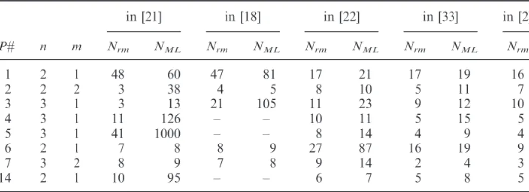
The selected results for Table 3 are from papers based on reduction-type methods. We observe that the use of P-DIP, when solving the reduced optimization problem, significantly reduces Nrm and NML, especially when compared with our
previous reduction-type methods based on penalty techniques. The comparison with other reduction-type methods is also favourable to our proposal. The use of the trial point ‘acceptance condition’ (AC-sip) in the filter methodology results in a significant reduction of multi-local procedure calls. Further, the use of a filter method allows the full Newton step to be taken more often. Another advantage related with the proposed P-DIP filter line search method is that no parameters are required to be updated during both iterative cycles – the inner cycle, aiming to obtain Table 1. Computational results.
P# n jTj f Nrm NML NIP
1 2 1 2.51381E001 5 6 9
1(1) 1 2.51383E001 6 7 9
2 2 1 2.61803Eþ000 2 3 9
2(1) 1 1.94466E001 3 4 8
2(2) 1 1.94466E001 2 3 8
3 3 1 5.33469Eþ000 3 4 9
3(1) 1 5.33469Eþ000 3 4 9
3(2) 1 5.33469Eþ000 3 4 9
4 3 1 6.49049E001 6 7 9
5 3 1 4.30118Eþ000 15 16 7
6(1) 2 1 1.07422
Eþ002 3 4 9
6(2) 1 1.07422Eþ002 2 3 9
7 3 2 1.00001Eþ000 3 4 9
7(1) 2 1.00001Eþ000 3 4 9
14 2 1 2.20000Eþ000 3 4 9
14(2) 1 2.20000Eþ000 2 3 9
Table 2. Results from other methods.
in [12] in [13] in [24] in [23] in [43]
P# n m Nit Nfeval Nit CPU Nit Nit CPU Nit Nfeval
2 2 2 2 22 10 0.13 7 7 0.13 7 20
3 3 1 5 39 9 0.17 4 9 0.17 3 36
6 2 1 3 26 20 0.28 6 5 0.11 5 25
14 2 1 – – 7 0.05 3 6 0.09 3 19
an approximate solution of the reduced finite problem, and the outer cycle, to find the SIP solution.
Future developments will address the use of the sparse symmetric indefinite linear solver MA27 from Harwell Subroutine Library to solve the system (12) in order to improve efficiency. A dynamic updating of the tolerancesIP1 andIP2 (depending on the iteration counterk) is now under investigation.
Acknowledgements
The authors wish to thank two anonymous referees for their careful reading of the manuscript and their valuable comments and suggestions.
References
[1] A. Ben-Tal, M. Teboule, and J. Zowe,Second order necessary optimality conditions for semi-infinite programming problems, Lecture Notes Control Inform. Sci. 15 (1979), pp. 17–30.
[2] I.D. Coope and G.A. Watson, A projected Lagrangian algorithm for semi-infinite
programming, Math. Progr. 32 (1985), pp. 337–356.
[3] M.F.P. Costa and E.M.G.P. Fernandes, Practical implementation of an interior point
nonmonotone line search filter method, Int. J. Comput. Math. 85 (2008), pp. 397–409.
[4] M.F.P. Costa and E.M.G.P. Fernandes, A three-D filter line search method within an
interior point framework, Proceedings of 2008 International Computational and Mathematical Methods in Science and Engineering, Salamanca, Spain, ISBN: 978-84-612-1982-7, 2008, pp. 173–187.
[5] A.S. El-Bakry, R.A. Tapia, T. Tsuchiya, and Y. Zhang,On the formulation and theory of the Newton interior-point method for nonlinear programming, J. Optim. Theory Appl. 89 (1996), pp. 507–541.
[6] R. Fletcher and S. Leyffer,Nonlinear programming without a penalty function, Math. Progr. 91 (2002), pp. 239–269.
[7] M.A. Goberna and M.A. Lo´pez (Eds.), Semi-Infinite Programming. Recent Advances,
Nonconvex Optimization and Its Applications, Vol. 57, Springer-Verlag, Kluwer Academics Publishers, Dordrecht, The Netherlands, 2001.
Table 3. Results from other reduction methods.
in [21] in [18] in [22] in [33] in [2]
P# n m Nrm NML Nrm NML Nrm NML Nrm NML Nrm
1 2 1 48 60 47 81 17 21 17 19 16
2 2 2 3 38 4 5 8 10 5 11 7
3 3 1 3 13 21 105 11 23 9 12 10
4 3 1 11 126 – – 10 11 5 15 5
5 3 1 41 1000 – – 8 14 4 9 4
6 2 1 7 8 8 9 27 87 16 19 9
7 3 2 8 9 7 8 9 14 2 4 3
14 2 1 10 95 – – 6 7 5 8 5