High speed rail transport valuation and policy decisions

WORKING PAPER SERIES

Universidade dos Açores Universidade da Madeira

CEEAplA WP No. 15/2008

High Speed Rail Transport Valuation and

Policy Decisions

Pedro Pimentel

José Azevedo-Pereira

Gualter Couto

High Speed Rail Transport Valuation and Policy

Decisions

Pedro Pimentel

Universidade dos Açores (DEG)

e CEEAplA

José Azevedo-Pereira

Departamento de Gestão e CIEF,

Instituto Superior de Economia e Gestão

Gualter Couto

Universidade dos Açores (DEG)

e CEEAplA

Working Paper n.º 15/2008

Novembro de 2008

Novembro de 2008

RESUMO/ABSTRACT

High Speed Rail Transport Valuation and Policy Decisions

The present paper investigates the process of decision making regarding the

optimal timing to invest in the high speed rail (HSR) project, under uncertainty,

using the real options analysis (ROA) framework. It’s developed a continuous

time framework that allows a solution to the problem concerning the optimal

timing to invest and to value the impact of the option to defer in the overall

valuation of the project, with multiple uncertainty factors. Besides considering a

stochastic demand, the effect of uncertainty in the investment’s expenditure and

over the benefit per user is incorporated in a model with three stochastic

variables. The modelling approach used is based on the differential utility

provided to railway users by the HSR service.

Keywords: Real Options, Uncertainty, Timing, Waiting, Investment, High

Speed Rail.

JEL classification: D81, D83, D92.

Pedro Pimentel

Departamento de Economia e Gestão

Universidade dos Açores

Rua da Mãe de Deus, 58

9501-801 Ponta Delgada

José Azevedo-Pereira

Departamento de Gestão

Instituto Superior de Economia e Gestão

Universidade Técnica de Lisboa

R. Miguel Lupi,

1249-078 Lisboa

Gualter Couto

Departamento de Economia e Gestão

Universidade dos Açores

Rua da Mãe de Deus, 58

9501-801 Ponta Delgada

Pedro Miguel PimentelË University of the Azores

Business and Economics Department, CEEAplA,

R. Mãe de Deus, 9500 Ponta Delgada, Portugal, ppimentel@notes.uac.pt

José Azevedo-Pereira ISEG

Universidade Técnica de Lisboa Department of Management

R. Miguel Lupi, 1249-078 Lisboa, Portugal, jpereira@iseg.utl.pt

Gualter Couto University of the Azores,

Business and Economics Department, CEEAplA

R. Mãe de Deus, 9500 Ponta Delgada, Portugal, gcouto@notes.uac.pt

This draft: May 2008

ABSTRACT

The present paper investigates the process of decision making regarding the optimal timing to invest in the high speed rail (HSR) project, under uncertainty, using the real options analysis (ROA) framework. It’s developed a continuous time framework that allows a solution to the problem concerning the optimal timing to invest and to value the impact of the option to defer in the overall valuation of the project, with multiple uncertainty factors. Besides considering a stochastic demand, the effect of uncertainty in the investment’s expenditure and over the benefit per user is incorporated in a model with three stochastic variables. The modelling approach used is based on the differential utility provided to railway users by the HSR service.

Keywords: Real Options, Uncertainty, Timing, Waiting, Investment, High Speed Rail. JEL classification: D81, D83, D92.

Ë

1. Introduction

New approaches about investments under uncertainty suggest new valuation frameworks, given the ineffectiveness of the traditional approach of investments’ evaluation in unstable environment. The real option analysis (ROA) introduces new perspectives about the impact of uncertainty in a projects value (Dixit and Pindyck, 1994).

The exposure to several uncertainty factors confers value to flexibility. High levels of uncertainty increase the options’ value. This effect comes from the potential gains or the limitation of eventual losses, case the project goes through or not, as a result of an active management in an uncertain environment (Trigeorgis, 1996).

The work of Pimentel et al. (2007) will be the starting point to study the option to defer with multiple uncertainty factors, enabling a deeper analysis of the HSR investments opportunity value and the optimal timing to invest, regarding several uncertainty effects.

The decision to invest instead of delay will be obtained regarding the uncertainty that surrounds the demand level for the new HSR service, the demand expenditures and the benefits. Although the demand variable represents the main source of uncertainty (Rose, 1998), the developed model will simultaneously measure the impact of the other two uncertainty variables in the optimal investment decision. All stochastic variables follow a geometric Brownian motion process.

Considering that the government is the owner of the project, the investment decision could be seen as an economic welfare problem, in witch the utility balance of two similar rail services is carried out. The valuation framework is based on the utility gain by the citizens that use the new HSR service comparatively with a similar service in conventional rail.

2. Literature Review

The literature regarding the practical importance on a new investment’s valuation method was based on the study of the option to defer. Tourinho (1979) was one of the first researchers to show that the possibility of deferring the natural resources reserve’s operations (such as crude oil) could be studied and valuated as an option. Titman (1985) analyzed a building’s construction of 6 or 9 apartments, in a certain period or in the

following period, having concluded that the value of an unoccupied property is composed by the value of its immediate use, plus the value of the option to defer and converting it into a future better alternative. The empirical study on 2.700 real-estate transactions done in Seattle, enabled Quigg (1993) to find an evidence about the explicative capacity of the ROA’s model over the transaction prices and also the fact that market prices reflect a benefit for the optimal time-to-built of urban properties.

Paddock et al. (1988) show that the value of the option to defer the oil reserve’s operation may be a significant proportion of the total value regarding the exploration’s rights, especially when the present and expected conditions turn unprofitable the development of the oil fields. However, Copeland and Antikarov (2003), have questioned, at some extent, the relevancy of these developments, stating that the value of the option to defer seemed itself insufficient to justify the prices paid by the exploration’s rights. Probably, the prices paid include the value of other options incorporated in the investment opportunity, but not considered in Paddock et al. (1988)’s research.

The timing to invest has known theoretical developments when McDonald and Siegel (1986) developed a rule to determine the optimal timing to invest when the projects’ value and the investment’s expenditure are both stochastic. Simultaneously, they have quantified the lost value when the investment is done in a suboptimal period. Bjerksund and Ekern (1990), in a similar exercise, have studied an analytical solution to valuate the flexibility of deferring an oil field development when the output price, follows a geometric Brownian motion process. Quigg (1993) has also constructed a model to valuate the perpetual option of constructing an optimal building in an optimal timing, incorporating two uncertainty factors: the construction’s expenditure and the price of the constructed building. Mauer and Ott (1995) incorporated uncertainty in the maintenance operational costs and the taxes effect, in the decision of replacing an investment.

Meanwhile, Lee (1988), after specifying three models in order to analyze the optimal timing of three distinct investments (equipment replacement, property’s developments and commercialization of a new product), has found empirical evidence that the valuation of the option to defer depends on the crucial choice of the stochastic process that drives the project’s value.

Recently, Couto (2006) has investigated the option to defer the choice of optimal relocation using a poisson process for the localization’s efficiency measure. The author has derived optimal investment’s strategies considering different distribution functions, as the exponential-truncate function, which avoids the existence of leaps in the dimension’s efficiency arbitrarily high, and the gamma function, which enables the use of more than one uncertainty factor.

Apart from the existence of some research about real options analysis focusing in the transports investments (Rose, 1998; Brandão, 2002; Smit (2003); Salahaldin and Granger, 2005; and Pereira et al. 2006), the work of Bowe and Lee (2004) seems pioneer in the analysis of a railway project. Nevertheless, Bowe and Lee (2004), compute the option’s value using numerical solutions provided by binomial analysis. Related to analytical developments regarding the ROA’s application to railways investment, Pimentel et al. (2007) develops a model to valuate HSR project with stochastic demand. Most of the theoretical research work with analytical solutions deal with no more than 2 stochastic variables in a perpetual time horizon. In relation to Pimentel et al. (2007), this paper introduces two more stochastic variables, enabling the assessment of their impact in the valuation model.

3. Investments Valuation using ROA Framework

Following the developments of Pimentel et al. (2007), the demand level x (number t

of HSR passengers) for the new service is the main source of uncertainty regarding the HSR project. This uncertainty will be described by the following geometric Brownian motion process: x t x t x t xdt xdw dx =µ +σ (1)

In equation (1), µx and σx represent the growth rate and the standard deviation of

the demand for the HSR service. We assume that both parameters are constant in time. The Wiener process w has a zero mean and standard deviation _x σ_x dt.

With the purpose of measuring the impact of other uncertainty factors, ROA’s model will be developed in order to embrace uncertainty regarding the investment’s expenditure and the benefits for users. Besides demand, each one of the remaining

uncertainty factors follows a geometric Brownian motion process (McDonald and Siegel, 1986; Rose, 1998; Marathe and Ryan, 2005; Paxson and Pinto, 2005 and Pereira

et al., 2006. In the continuous time approach will be assumed that the option to defer is

unlimited in time (T =∞) and that the investment, once implemented, produces perpetual benefits.

Without a portfolio of spanning assets, the challenge relies on the optimal stopping problem in the dynamic programming language. In the continuation region the optimal decision is to defer. In the stopping region the optimal decision is to implement the investment. Thus, it’s important to find the critical value that delimits both regions, for a given discount rate ρ.

The investments in this sector are usually carried out by the Government, given the huge amount of money needed and the monopoly characteristic. Therefore, we may consider that the HSR project belongs to all the potential users which are part of an economy and that may use, without restraints, the existent services offered by the conventional railway. In these conditions, the Government may be willing to invest if the benefits from the HSR service, regarding the conventional one, justify the investment’s expenditure, which is almost sunk cost. This framing enables to consider hypothetically that each potential user of the HSR assumes his/her share of investment’s expenditure and the according operating costs per user.

The main benefit of the HSR is associated to the travel time reduction, (Wilson, 1986). It is assumed that the combination of the value of time spent in a trip η and the price p from the according fare represent the travel cost ψ. The value of time spent in a trip η is given by the functional form βxδtβ (Owen and Phillips, 1987, and

Wardman, 1994). Consequently, the scale parameter β0 and β2 will reflect the

relationship between demand x and the value of travel time for conventional railway t

0

η and HSR η2 accordingly. Analytically β will be given by:

( )

δβ η β ₌ − t t x x (2)

Similarly, the price p is given by the functional form α δα

t

x (Owen and Phillips, 1987). Analytically the scale parameter α between the HSR demand x and the railway t

( )

δα α₌ − t t x x p (3)

The users will only choose to travel in the HSR if they could at least maintain their utility function, at the same level as the one they had in the conventional service. Otherwise, it will always be better to pay the fare for the conventional service even if they spend more time travelling.

The fact that the investment has an infra-structuring nature of governmental scale, allows to be considered as an economic welfare problem, based upon the equilibrium between the utility function of two similar services.

The valuation model relies on the equilibrium of the utility function and considers the existence of variable ω and fixed ϕ operating costs. The model also considers the time-to-build effect n and incorporates the existence of an elasticity between the value of travel time and the demand level δ_β, as well as a cross elasticity between the HSR demand and the conventional service fare δ_α.

Like in Pimentel et al. (2007), when the demand follows the stochastic process in equation (1) and given the actual demand level and discount rate ρ, the value of the project v is determined through the maximization of the function:

( )

t x E

[

e

(

A

( )

x B

( )

x F

( )

x C D

)

]

v , = _x −ρτ _tc ∗ θβ + _tc ∗ θα + _tc ∗ + _tc + (4) With,

(

)

( ) 2 2 2 1 2 1 2 0 2 2 2 2 x x x n tc x x e A σ θ σ θ θ µ ρ β β β β β ρ σ θ θ θ µ β β β + − − − = ⎟ ⎠ ⎞ ⎜ ⎝ ⎛ _{+ − −} (5) ( ) 2 2 2 1 2 1 0 2 2 2 2 x x x n tc x x e B σ θ σ θ θ µ ρ α α α α ρ σ θ θ θ µ α α α + − − = ⎟ ⎠ ⎞ ⎜ ⎝ ⎛ _{+ − −} (6) ρ ϕ ρn tc e C − − = (7) γ − = D (8)

( ) x n tc x e F µ ρ ω µ ρ − − = − (9) β β δ θ = 1+ (10) α α δ θ = 1+ (11)

and under the following condition

(

1

)

0 2

1 − 2>

−

−θµx θ θ σx

ρ , that assures the existence of a future optimal timing to invest. This condition imposes that the demand growth rate must be lower than discount rate, thus providing a rational economic interpretation to the model developments.

3.1. Investment Valuation using Real Options Framework with Demand and Investment’s Expenditures Stochastic

Based on the early developments and assumptions, we may extend the model in order to contemplate another uncertainty factor besides the demand for the HSR service. Suppose that the investment expenditure is influenced by uncertainty throughout time. This assumption could be relevant for projects whose investment assets are subject to price variations throughout time, as in case of assets technologically developed.

In these scenarios the investment’s value is expressed as a function of both variables

(

x, γ

)

v , so that it is necessary to find the curve of critical values

(

x*, γ*

)

which delimits the region of values of

(

x,γ

)

in which it’s suboptimal to invest, from the region of values for which is optimal to invest.

3.1.1. Optimal Timing to Invest

Consider that the demand for the HSR service follows a geometric Brownian motion process described by equation (1) and that the investment’s expenditure also follows an identical process described by,

γ γ γγ σ γ µ γ dt dw d t = t + t (12)

enabling the existence of a correlation effect between both variables,

(

dwdw

)

corr dt

E x γ = x,γ , perhaps due to common macroeconomic shocks (McDonald and

Siegel, 1986 and Dixit and Pindyck, 1994). Notice that in this specific case, once is optimal to invest, the uncertainty in the investment’s expenditure value becomes irrelevant.

In this context, the total net benefits value resultant from investment Z

( )

x , in the stopping region results from equation (4), in *

x

x≥ , so that:

( )

x Atcx Btcx Ftcx Ctc

Z = θβ + θα + +

(13) with A , _tc B , _tc C and _tc F given by (5), (6), (7) and (10), accordingly. _tc

However, the same simplicity no longer exists when we want to know the investment’s value in *

x

x< , once it depends on x and γ, both stochastic. Recall that we hold an investment opportunity, which doesn’t produce any cash-flow until the moment in witch investment is implemented. The only value that maintains the opportunity open comes exclusively from the project’s own value, given by function

( )

x,γ

v , which include the value of the option to defer .

Therefore, at the continuation region (when it’s still suboptimal to invest) Bellman’s equation is given by:

( )

dv E vdt=

ρ (14)

which denote that in a time interval dt the total rate of return from the investment opportunity vdtρ is equal to the rate of return expected from its own value increase throughout time.

If we expand dv using the Itô lemma for two stochastic variables we have, according to Neftci (2000):

( )

( )

_⎥ ⎦ ⎤ ⎢ ⎣ ⎡ ∂ ∂ ∂ + ∂ ∂ + ∂ ∂ + ∂ ∂ + ∂ ∂ = γ γ γ γ γ γ x dxd v d v dx x v d v dx x v dv 2 2 2 2 2 2 2 2 2 1 (15)

Replacing in (15) dx and d given, accordingly, by (1) and (12), and considering γ

( )

dw =0

( )

dt x v x corr v x v x dt v dt x v x dv E x x x x ⎥ ⎦ ⎤ ⎢ ⎣ ⎡ ∂ ∂ ∂ + ∂ ∂ + ∂ ∂ + ∂ ∂ + ∂ ∂ = γ γ σ σ γ γ σ σ γ γ µ µ γ γ γ γ 2 , 2 2 2 2 2 2 2 2 2 2 1 (16) Replacing equation (16) in (14) and dividing all for dt , we obtain the partial differential equation, which satisfies the investment’s value function v

(

x, γ

)

at the continuation region: 0 2 2 1 2 , 2 2 2 2 2 2 2 2 _{− =} ∂ ∂ + ∂ ∂ + ⎥ ⎦ ⎤ ⎢ ⎣ ⎡ ∂ ∂ ∂ + ∂ ∂ + ∂ ∂ v v x v x x v x corr v x v x x x x x σ γ _γ σ σ γ _γ µ µ γ _γ ρ σ _{γ γ γ γ} (17) With the following boundary conditions:

1. Initial condition:

( )

0,γ =0

v ₍₁₈₎

2. Value matching condition:

( )

γ =

( )

−γ =

( )

θβ +

( )

θα +

( )

+ −γ tc tc tc tc x B x F x C A x Z x v , , with x= x∗ and γ =γ∗ (19) 3. Smooth-pasting conditions:

( )

( )

tc tc tc x x Z x A x B x F v , = ′ = β−1+ θω−1+ α θ β θ θ γ , with x= x∗ and γ =γ∗ (20) and

( )

,γ = ′

( )

,γ =−1 γ x v x v , with x= x∗ and γ =γ∗ (21) Solving the partial differential equation (17) along with the boundary conditions (18) to (21) besides delimiting the region of the investment’s critical value constitutes the solution for the investment’s value function v

(

x, γ

)

at the continuation region.

However, the complexity of partial differential equation (17) doesn’t allow an analytical solution. Only numerical methods capable of solving problems of free-limits for elliptic partial differential equations could solve it, as pointed out by Dixit and Pindyck (1994).

Aiming to obtain analytical developments for the investment’s value solution, we may consider θ=θ_β =θ_ω, 0Ftc = and Ctc =−lγ . The first assumption related to

equality between the HSR demand/value of travel time elasticity and the HSR demand/conventional service fare cross elasticity. The second assumption comes from the possibility of neglecting the variable operating costs considering the operational characteristics of the project. The last assumption formulates the fixed operating costs as a proportion ( l ) from the investment’s expenditure. These simplifications assure the existence of natural homogeneity in the model, explored by McDonald and Siegel (1986), allowing its reduction to a single dimension.

The natural homogeneity concerning this specific problem results from the fact that any constant multiplied by x and by θ γ, simply affects the total net present benefit value resultant from investment Z

( )

x and the investment expenditure γ in the same proportion of the constant.

We may rewrite the project’s value function, such as:

(

γ

)

(

θ γ

)

, , k kf x kx v = (22) Considering γ 1 =

k and after simplifying, we have:

(

)

_⎟⎟ ⎠ ⎞ ⎜ ⎜ ⎝ ⎛ = ⎟ ⎟ ⎠ ⎞ ⎜ ⎜ ⎝ ⎛ = γ γ γ γ γ f xθ f xθ x v , , 1 (23)

in which f is a function to be determined.

With:

γ

θ

x

q= (24)

The unknown function f can be determined from successive differentiations of

(

x, γ

)

v given by equation (23). Consider f ′ and f ′′ the first and second derivatives,

accordingly, of function f . The successive derivatives of v

(

x, γ

)

come: 1. First derivative of v

(

x, γ

)

with respect to x :

( )

1 1 − − _′ = ∂ ∂ _θ θ _θ θ x q f x x v (25) 2. First derivative of v

( )

x,γ with respect to γ :

( )

q x f

( )

q f v _{= − ′} ∂ ∂ γ γ θ (26)

3. Second derivative of v

( )

x,γ with respect to x :

( ) (

)

( )

⎥ ⎥ ⎦ ⎤ ⎢ ⎢ ⎣ ⎡ ′ − + ′′ = ∂ ∂ − − q f x q f x x v 2 2 2 2 2 1 θ θ θ γ θ θ ₍₂₇₎

4. Second derivative of v

(

x, γ

)

with respect to γ:

( )

q f x v _{= ′′} ∂ ∂ 3 2 2 2 γ γ θ (28) and

5. Second cross derivative v

( )

x,γ with respect to x and γ:

( )

⎥ ⎥ ⎦ ⎤ ⎢ ⎢ ⎣ ⎡ ′′ ⎟ ⎟ ⎠ ⎞ ⎜ ⎜ ⎝ ⎛ − = ∂ ∂ ∂ − q f x x x v 2 1 2 γ θ γ θ θ (29)

Replacing equations (25) to (29) in the partial differential equation (17), dividing all elements for γ before simplifying, we get the following ordinary differential equation:

[

]

( )

(

1

)

( )

(

)

( )

0 2 1 2 2 1 2 2 , 2 2 2 ′ _{− − =} ⎥⎦ ⎤ ⎢⎣ ⎡ _{+ − −} + ′′ − + x corrx q f q x x qf q f q xθ σγ σ σγ γθ µθ σ θθ µγ ρ µγ σ (30) which satisfies the following boundary conditions:

1. Initial contition:

( )

0 =0

f (31)

2. Value matching condition:

( ) (

q =q A +B

)

−l−1 f tc tc , for ∗ = q q (32) and, 3. Smooth-pasting condition:

( ) (

q Atc Btc

)

f′ = + , for q= q∗ (33) The solution of equation (30) is given by:

( )

1 2 2 1 s s q b q b q f = + (34)

where s1 and s2 are the roots from the quadratic equation:

[

]

(

)

(

1

)

(

)

0 2 1 1 2 2 1 2 , 2 2 2 − − = ⎥⎦ ⎤ ⎢⎣ ⎡ _{+ − −} + − − +σ_γ σ σ_{γ γ}θ µθ σ θ θ µ_γ ρ µ_γ θ σx x corrx ss x x s (35) given by,

(

)

2 2 2 2 2 1 2 2 1 2 1 q q q q q q s σ µ ρ σ σ µ µ σ ⎟ + − _γ ⎠ ⎞ ⎜ ⎝ ⎛ ₋ + ⎟ ⎠ ⎞ ⎜ ⎝ ⎛ ₋ = (36) and

(

)

2 2 2 2 2 2 2 2 1 2 1 q q q q q q s σ µ ρ σ σ µ µ σ ⎟ + − _γ ⎠ ⎞ ⎜ ⎝ ⎛ ₋ − ⎟ ⎠ ⎞ ⎜ ⎝ ⎛ ₋ = (37) with 2 , 2 2 2 2σ σ_{γ γ}θ σ_γ θ σ σq = x − x corrx + and µ =µθ+ σ θ

(

θ−1

)

−µγ 2 1 2 x x q . As 2 2 s q

b tends to the infinity when q tends to zero, according to the initial condition (31) and f

( )

q needs to be limited when q→0, 0b₂= . Thus equation (34) becomes,

( )

1 1 s q b q f = (38)

Using the equation (38) and the value matching condition

( )

* = *

(

+

)

− −1 l B A q q

f tc tc , we find the coefficient 1

(

)

1 1

* * 1 * 1 s s tc tc s q lq B A q b = − + − − − − ,

concluding that the solution of equation (30) is implicitly given by the equation:

( )

[

*1 1

(

)

* s1 * s1

]

s1 tc tc s q q lq B A q q f = − + − − − − (39)

The value of q* which maximizes f

( )

q is given by:

( )

(

)

⎥ ⎦ ⎤ ⎢ ⎣ ⎡ − ⎥ ⎦ ⎤ ⎢ ⎣ ⎡ + + = 1 1 1 1 * s s B A l q tc tc (40)

The critical value q* computed by the model, represents the optimal ratio

γ

θ

x

, that when achieved justifies the immediate implementation of the project. This solution preserves the utility function equilibrium between the HSR and conventional railway service for its users.

From the analytical solution of q* it’s possible to find the critical demand value x* for a known investment’s expenditure value γ, in a specific moment in time. In this case, the critical demand value may be achieved using equations (24) and (40), such as:

( )

(

) (

)

θ γ 1 1 1 * 1 1 ⎥ ⎦ ⎤ ⎢ ⎣ ⎡ − + + = s s B A l x tc tc (41)

This solution deals with the uncertainty effect from both investment’s expenditure and demand.

Case it’s expected a positive growth in the investment’s expenditure, this model shall support an anticipation of the optimal timing to invest, regarding the optimal timing achieved when there isn’t uncertainty upon investment’s expenditure. The investment’s expenditure increase under uncertainty may justify an anticipation of the project’s implementation taking advantage from a lower investment’s expenditure (McDonald and Siegel, 1986).

3.2. Valuation of HSR Investment using ROA Framework

Considering equation (39), for a known value of q , in t=0, the value of investment’s opportunity measured in proportion to the investment’s expenditure, when

*

q

q< and q≥q* is given by, accordingly:

( )

_*

[

(

)

* 1

]

1 − − + ⎟⎟ ⎠ ⎞ ⎜⎜ ⎝ ⎛ = A B q l q q q f tc tc s (42) and

( ) (

[

)

1s1 s1 s1

]

s1 tc tc B q lq q q A q f = + − − − − − (43)

Replacing the critical value q , given by equation (40), in the second part of the *

right hand side of equation (42) and simplifying we may rewrite the solution, such as:

( )

( )

(

)

(

)

⎪ ⎪ ⎪ ⎪ ⎩ ⎪⎪ ⎪ ⎪ ⎨ ⎧ ≥ − − + < ⎥ ⎦ ⎤ ⎢ ⎣ ⎡ − + ⎟⎟ ⎠ ⎞ ⎜⎜ ⎝ ⎛ = * 0 * 0 1 * 1 1 1 1 q q for l q B A q q for s l q q q f tc tc s (44)

In a specific moment in time and knowing the investment’s expenditures γ, the project’s value may be achieved considering v

( )

x,γ =γ f

( )

q . Hence,

( )

( )

(

)

(

)

[

]

⎪ ⎪ ⎪ ⎪ ⎩ ⎪⎪ ⎪ ⎪ ⎨ ⎧ ≥ − − + < ⎥ ⎦ ⎤ ⎢ ⎣ ⎡ − + ⎟⎟ ⎠ ⎞ ⎜⎜ ⎝ ⎛ = * * 1 * 1 1 1 , 1 q q for l q B A q q for s l q q x v tc tc s γ γ γ (45)

Equation (45) incorporates the value of the option to defer, resultant from waiting for new information about demand and investment’s expenditure while the critical value

*

q it’s not reached. As soon as the critical value *

q is reached, it becomes optimal to

invest and receive the NPV, given by

[

(

Atc +Btc

)

q−l−1

]

γ.

Even though this model has been developed with constraints which limit its wideness from all real circumstances that involve the HSR investment, it assesses the impact from investment’s expenditures uncertainty in the project’s value.

3.3. Investments’ Valuation using Real Options Framework with Demand, Benefit and Investment’s Expenditures Stochastic

The previous model incorporates the impact of the investment’s expenditure uncertainty in the project’s valuation, under the assumption that θ =θ_β =θ_α, 0F_tc =

and C_tc =−lγ.

Until now the total benefits

(

β0 −β2 +α0

)

xθ resultant from the project were only

influenced by demand uncertainty. Although the benefit, represented by

(

β0 −β2 +α0

)

is influenced by the elasticity parameter θ, it remains deterministic in nature.

In this context, it’s worthwhile to consider the inclusion of uncertainty on the benefit resultant from the project, R=

(

β₀ −β₂ +α₀

)

. Implicitly, R measures the travel cost reduction per user, resulting from using the HSR service comparatively to the conventional railway service.

With the inclusion of a third stochastic variable the project’s value is now expressed regarding v

(

x,R,γ

)

. Now it’s necessary to find the surface of critical values

(

* * *

)

, ,R γ

x which delimits the region of

(

x,R,γ

)

values in which is suboptimal to invest, from the region of values in which is optimal to invest.

As in the developments with two stochastic variables, the solution in the continuation region for v

(

x,R,γ

)

is achieved solving, through numerical methods, the partial differential equation with its boundary conditions. The solution for this equation is even more complex than the one for equation (17).

However, and similarly to the presented developments with two stochastic variables, the conditions θ =θβ =θα, 0Ftc = and Ctc =−lγ associated to some features and

proprieties of the problem allow a closed form solution.

3.3.1. Optimal Timing to Invest

Consider that the demand for the HSR service and the investment’s expenditure follow a geometric Brownian motion process described by equations (1) and (12), accordingly. The benefit resultant from the project also follows an identical process:

R t R t R t Rdt Rdw dR =µ +σ (46)

Considering that the benefit resultant from the project is represented by:

0 2 0 β α β − + = R ₍₄₇₎

the total benefits may be represented by the function P ,

(

x R

)

, with:

(

)

θ

Rx R x

P , = (48)

Since x and R are both stochastic, its product will also be stochastic. Through the

Itô lemma, we may reduce these two stochastic variables into one:

( )

( )

_⎥ ⎦ ⎤ ⎢ ⎣ ⎡ ∂ ∂ ∂ + ∂ ∂ + ∂ ∂ + ∂ ∂ + ∂ ∂ = dxdR R x P dR R P dx x P dR R P dx x P dP 2 2 2 2 2 2 2 2 2 1 (49)

Applying the function P ,

(

x R

)

derivatives, replacing dx and dR given by (1) and (46), accordingly, in equation (49) and after some simplifications, we have:

(

)

corr Pdt

[

dw dw

]

P dP θµx µR θθ σx θσxσR xR⎥⎦ + θσx x+σR R ⎤ ⎢⎣ ⎡ _{+ + − +} = , 2 1 2 1 (50) in which corrx,Rdt=E

(

dwxdwR

)

.

The growth rate and variance of P , µP and

2

P

σ , are, accordingly, given by:

(

)

x x R xR R x P corr, 2 1 2 1_{θ θ σ θσ σ} µ θµ µ = + + − + (51) and 2 , 2 2 2 2 _{x R xR R} x P θ σ θσ σ corr σ σ = + + ₍₅₂₎

Hence, the project’s value is now expressed regarding two variables v

(

P,γ

)

, which can be solved similarly to the previous model with demand and investment’s expenditure both stochastic.

Also in this case, from the investments optimal implementation, the investment’s expenditure uncertainty becomes irrelevant. The value of the total net benefits resultant from investment Z

( )

P in the stopping region (P≥ P∗), comes:

( )

P PAtct Ctc

Z = + , for P≥ P∗ (53)

with C given by (7) and tc

( ) P n tct P e A µ ρ ρ µ − = − (54)

As long as the optimal timing to invest is not reached, P<P*, the investment’s expenditure uncertainty remains relevant, with the project’s value staying dependent on two stochastic variables, P and γ.

Considering that corrP,_γdt=E

(

dwPdw_γ

)

, the project’s value function v

(

P,γ

)

satisfies a partial differential equation similar to equation (17):

0 2 2 1 2 , 2 2 2 2 2 2 2 2 _{− =} ∂ ∂ + ∂ ∂ + ⎥ ⎦ ⎤ ⎢ ⎣ ⎡ ∂ ∂ ∂ + ∂ ∂ + ∂ ∂ v v P v P P v P corr v x v P P P P P σ γ _γ σ σ γ _γ µ µ γ _γ ρ σ _{γ γ γ γ} (55) with the following boundary conditions:

1. Initial condition:

( )

0,γ =0

v ₍₅₆₎

2. Value matching condition:

(

P γ

)

=Z

( )

P −γ =A P−lγ −γ v , tct , with ∗ = P P e γ =γ∗ (57) 3. Smooth-pasting conditions:

(

)

( )

tct P P Z P A v ,γ = ′ = , with P= P∗ e γ =γ∗ ₍₅₈₎ and

(

P,

)

=v′

(

P,

)

=−l−1 v_γ γ γ , with P= P∗ e γ =γ∗ (59) The equation’s solution (55) can only be determined through numerical methods. However, the natural homogeneity in the problem, allows once more its reduction to a single dimension.

Under the homogeneity condition we may rewrite the project’s value function as:

(

)

_⎟⎟ ⎠ ⎞ ⎜⎜ ⎝ ⎛ = ⎟⎟ ⎠ ⎞ ⎜⎜ ⎝ ⎛ = γ γ γ γ γ f P f P P v , , 1 (60)

in which f is again a function to be determined.

γ

P

g= ₍₆₁₎

the optimal decision depends only on the critical value g , which represents the optimal *

ratio between the total benefits and the investment’s expenditure.

The new unknown function f can be determined from successive differentiations

of v

(

P,γ

)

given by equation (60). Consider once more f ′ and f ′′ the first and second

derivatives, accordingly, of function f . The successive derivatives of v

(

P,γ

)

come: 1. First derivatives of v

(

P,γ

)

with respect to P :

( )

g f P v _{= ′} ∂ ∂ (62) 2. First derivatives of v

(

P,γ

)

with respect to γ:

( )

g P f

( )

g f v _{= − ′} ∂ ∂ γ γ (63)

3. Second derivatives of v

(

P,γ

)

with respect to P :

( )

γ 1 2 2 − ′′ = ∂ ∂ g f P v (64)

4. Second derivatives ofv

(

P,γ

)

with respect to γ:

( )

g f P v _{= ′′} ∂ ∂ 3 2 2 2 γ γ (65) and

5. Second cross derivatives v

(

P,γ

)

with respect to P and γ:

( )

₂ 2 γ γ P g f P v _{=− ′′} ∂ ∂ ∂ (66)

Replacing equations (62) to (66) in the partial differential equation (55), dividing all elements for γ and after simplifying, we achieve the following ordinary differential equation:

[

2

]

( )

[

]

( )

(

)

( )

0 2 1 2 , 2 2 _{+ −} ′′ _{+ −} ′ _{− − =} g f g f g g f g corrP P P P σγ σ σγ γ µ µγ ρ µγ σ (67)

To solve equation (67) the following boundary conditions are needed: 1. Initial condition:

( )

0 =0

f (68)

2. Value matching condition:

( )

g =gA −l−1 f tct , with ∗ = g g (69) and 3. Smooth-pasting condition:

( )

g Atct f′ = , with g= g∗ (70) Similar to the previous developments, equation (67) solution given by:

( )

1 2 2 1 u u g y g y g f = + (71)

The two roots (u and 1 u ) from the following quadratic equation: 2

[

2

]

(

1

)

[

]

(

)

0 2 1 , 2 2_{+ − − + − − − =} γ γ γ γ γ σ σ µ µ ρ µ σ σ_{P P} corr_P uu _P u (72)

are obtained by,

(

)

2 2 2 2 2 1 2 2 1 2 1 g g g g g g u σ µ ρ σ σ µ µ σ ⎟ + − γ ⎠ ⎞ ⎜ ⎝ ⎛ ₋ + ⎟ ⎠ ⎞ ⎜ ⎝ ⎛ ₋ = (73) and

(

)

2 2 2 2 2 2 2 2 1 2 1 g g g g g g u σ µ ρ σ σ µ µ σ ⎟ + − γ ⎠ ⎞ ⎜ ⎝ ⎛ ₋ − ⎟ ⎠ ⎞ ⎜ ⎝ ⎛ ₋ = (74) with , 2 2 2 2σ σ_{γ γ} σ_γ σ σg = P− P corrP + and µg =µP−µγ.

Based on the initial boundary condition (68) is possible to verify that when g→0,

( )

g

f shall also tend to zero, so that it’s necessary that y2 =0. The solution given by equation (71) comes now,

( )

1 1 u g y g f = (75)

The combination of equation (75) with the value matching condition,

( )

* ₌ * _{− −}1

l A g g

f _tct , determines the coefficient *1 1 * 1 * 1

1 u u tct u g g l A g y = − − − − − , so that the solution to the equation (67) is given by:

( )

[

*1 1 * u1 * u1

]

u1 tct u g g g l A g g f = − − − − − (76)

The function f

( )

g maximization occurs when g is given by: ∗

( )

⎥ ⎦ ⎤ ⎢ ⎣ ⎡ − ⎥ ⎦ ⎤ ⎢ ⎣ ⎡ + = 1 1 1 1 * u u A l g tct (77)

The critical value g represents the optimal ratio between the total benefits P and *

the investment’s expenditure γ, that when reached, justifies the immediate investment’s implementation. Similar to the previous model, this solution preserves the utility function equilibrium between HSR and conventional service for railway users.

From the analytical solution of *

g it’s possible to find the demand’s critical value

*

x , in a specific moment in time. For such, the investment’s expenditure γ and the benefit R , must both be known in this particular moment. In this case, the demand critical value can be obtained replacing

γ

P

g= in equation (77), such as:

( )

⎥ ⎦ ⎤ ⎢ ⎣ ⎡ − ⎥ ⎦ ⎤ ⎢ ⎣ ⎡ + = 1 1 1 1 u u A l P tct γ (78)

Considering P=Rxθ and R=

(

β₀ −β₂ +α₀

)

, known in a specific moment, we may rewrite the previous equation regarding the only unknown variable left, such as:

( )

θ γ 1 1 1 1 * 1 1 ⎥ ⎥ ⎦ ⎤ ⎢ ⎢ ⎣ ⎡ ⎥ ⎦ ⎤ ⎢ ⎣ ⎡ − ⎥ ⎦ ⎤ ⎢ ⎣ ⎡ + = − R u u A l x tct (79)

Similar to the model with stochastic demand and investment’s expenditure, this solution maintains consistent with the solution obtained by equation (41) under the same assumptions. The difference between both solutions – equations (41) and (79) – reflects the additional impact from the benefits ( R ) uncertainty.

The inclusion in the model of uncertainty upon the benefits R , leads to a longer waiting period of time until it’s optimal to invest, comparatively to the solution given by the previous model with two stochastic variables. This expected effect is contrary to the one obtained with the inclusion of uncertainty upon the investment’s expenditure γ . The uncertainty effect upon the benefits exposes the project even more to uncertainty, requiring more cautiousness regarding the investments’ implementation (Dixit and Pindyck, 1994).

Under opposite influences, case we include uncertainty upon the investment’s expenditure γ and upon benefits R , the net effect shall depend on the impact’s magnitude of each uncertainty variable.

3.3.2. Valuation of an HSR Investment using ROA Framework

Based on the previous developments, the investment’s opportunity value in proportion to the investment’s expenditure is obtained from equation (76), once the value of g , in t=0 is known. Analytically, we have:

( )

[

* 1

]

* 1 − − ⎟⎟ ⎠ ⎞ ⎜⎜ ⎝ ⎛ = A g l g g g f _tc u , for * g g< (80) and

( )

[

1u1 u1 u1

]

u1 tctg lg g g A g f = − − − − − , for * g g≥ (81)

The solution is achieved replacing the critical value g , given by equation (77), in *

the second part of the right hand side of equation (80) and simplifying, such as:

( )

( )

(

)

⎪ ⎪ ⎪ ⎪ ⎩ ⎪⎪ ⎪ ⎪ ⎨ ⎧ ≥ − − < ⎥ ⎦ ⎤ ⎢ ⎣ ⎡ − + ⎟⎟ ⎠ ⎞ ⎜⎜ ⎝ ⎛ = * * 1 * 1 1 1 1 g g for l g A g g for u l g g g f tct u (82)

with l=−Ctcγ−1 and C , tc u and 1 A given by (7), (73) and (54), accordingly. tct

Using the relation initially established, in which v

(

P,γ

)

=γ f

( )

g , the project’s value can be obtained if in a specific moment in time, the investment’s expenditure γ and the benefits R are both known. Hence, we have:

(

)

( )

(

)

[

]

⎪ ⎪ ⎪ ⎪ ⎩ ⎪⎪ ⎪ ⎪ ⎨ ⎧ ≥ − − < ⎥ ⎦ ⎤ ⎢ ⎣ ⎡ − + ⎟⎟ ⎠ ⎞ ⎜⎜ ⎝ ⎛ = * * 1 * 1 1 1 , 1 g g for l g A g g for u l g g P v tct u γ γ γ (83)

In the continuation region (while g is not reached) equation (83) incorporates the *

value of the option to defer, which represents the value resultant from waiting for new information about demand, travel cost and investment’s expenditure. When the critical value *

g is reached, the project with a NPV equal to

[

A_tctg− l−1

]

γ should be implemented immediately.

Such as in the model with demand and investment’s expenditure stochastic, this new model was also developed under constraints which may limit it from real circumstances that may involve HSR investment. Nonetheless, it’s useful to measure simultaneously the impact from investment’s expenditure and benefits uncertainties in the project’s value.

4. Numerical Example

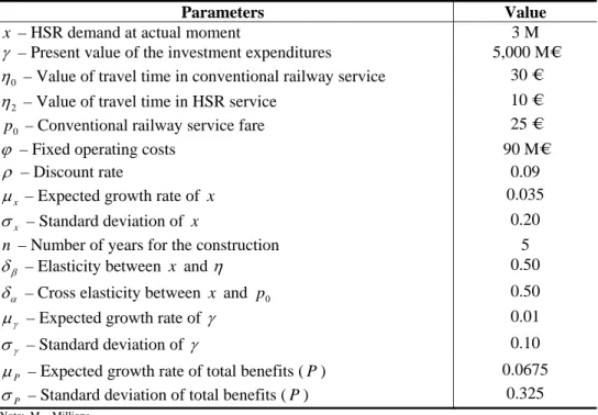
Table 1. Base-case parameters for the project

Parameters Value

x – HSR demand at actual moment 3 M

γ – Present value of the investment expenditures 5,000 M€

0

η – Value of travel time in conventional railway service 30 €

2

η – Value of travel time in HSR service 10 €

0

p – Conventional railway service fare 25 €

ϕ – Fixed operating costs 90 M€

ρ – Discount rate 0.09

x

µ – Expected growth rate of x 0.035

x

σ – Standard deviation of x 0.20

n – Number of years for the construction 5

β

δ – Elasticity between x and η 0.50

α

δ – Cross elasticity between x and p 0 0.50

γ

µ – Expected growth rate of γ 0.01

γ

σ – Standard deviation of γ 0.10

P

µ – Expected growth rate of total benefits ( P ) 0.0675

P

σ – Standard deviation of total benefits ( P ) 0.325

Note: M = Millions

Assume a project for the construction of a HSR line connection between two cities. The basic parameters are in Table 1. For simplicity, the variable operating costs is neglected and all correlations between variables are assumed to be zero. The conventional railway service operates in the same link. The new HSR service will reduce the travel time to one third comparatively to the conventional railway service.

Table 2 presents the HSR line investment valuation results for the base-case parameters.

The results, considering three uncertainty factors, suggest that the investment shall only be implemented when the project achieves an amount of annual benefits which represent a proportion equal or superior to 18.7% from the present value of the investment expenditures. At the present moment this ratio assumes a value of 2.7%, therefore the project shall not be implemented immediately. The investment opportunity value represents 64.32% of the investment’s expenditures present value, while the value of the option to defer assumes a proportion of 69.84%.

Table 2. Project valuation results

Output Value

∗

g – Critical ratio between total benefits and investment expenditures 0.1870

( )

_{< g}∗

g with g

f , – Investment Opportunity Value in percentage of the investment expenditures

64.32%

( )

_{≥ g}∗

g with g

f , – Net Present Value in percentage of the investment expenditures

-5.52%

( )

g

vod – Value of the Option do Defer in percentage of the investment expenditures

69.84%

∗

x – Critical demand for HSR service (n.º passengers) 10.898 M

( )

_{< g}∗

g with P

v ,γ , – Investment Opportunity Value 3,215.8 M€

( )

_{≥ g}∗

g with P

v ,γ , – Net Present Value -276.0 M€

( )

P,γ

vod – Value of the Option do Defer 3,491.8 M€

Considering that in a particular moment the present value of the investment’s expenditures assumes a value of 5,000 millions Euros, the optimal implementation of the project, at that moment, depends on the existence of a demand level for the HSR service equal or superior to 10.898 millions passengers. This critical demand value comes slightly superior in 2.21%, regarding the value obtained when only the uncertainty in the passengers’ volume is considered. At this moment, the project has a negative NPV of 276.2 millions Euros. However, this project shall not be abandoned, since the option’s value of implementing it in the future is 3,491.8 millions Euros. Thus, this investment opportunity is worth 3,215.8 millions Euros, if the option to defer its implementation stays open.

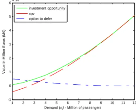
Figure 1. Investment’s opportunity value, NPV and value of the option to defer, for

the base case

1 2 3 4 5 6 7 8 9 10 11 12 -1 0 1 2 3 4 5 6x 10 4

Demand (xt) - Million of passengers

V a lu e in M illio n E u ro s ( M € ) investment opportunity npv option to defer

Figure 1 shows the growth of the investment’s opportunity value, NPV and value of the option to defer, towards the increase on the passenger’s number, throughout time.

Assuming an investment’s expenditures present value of 5,000€ millions Euros, the value of the option to defer becomes zero from the moment demand reaches a critical value of 10.898 millions of passengers. Once achieved this critical value, the optimal decision is the immediate implementation of the investment.

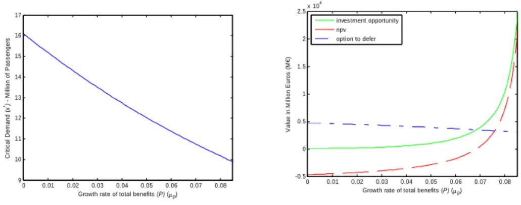
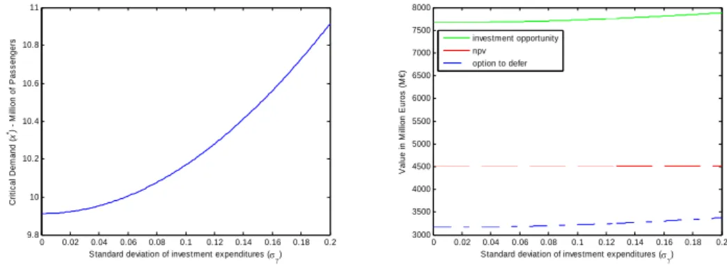
Figure 2. The impact of the growth rate of total benefits ( P )

0 0.01 0.02 0.03 0.04 0.05 0.06 0.07 0.08 9 10 11 12 13 14 15 16 17

Growth rate of total benefits (P) (µP)

C rit ic a l D e m a n d ( x *) - M ill io n of P a s s enger s 0 0.01 0.02 0.03 0.04 0.05 0.06 0.07 0.08 -0.5 0 0.5 1 1.5 2 2.5x 10 4

Growth rate of total benefits (P) (µP)

V a lue i n M il li on E u ro s ( M €) investment opportunity npv option to defer

Figure 2 to Figure 15 show the sensibility of the critical demand level, investment’s opportunity value, net present value, and the value of the option to defer regarding the variation of some parameters. The critical demand level presents a direct relation with the discount rate (Figure 4), standard deviation of total benefits (Figure 5), standard deviation of investment’s expenditures (Figure 6), standard deviation of demand (Figure 7) and time-to-built (Figure 8). The growth rate of total benefits (Figure 2), growth rate of investment’s expenditures (Figure 3) and the value of travel time reduction (Figure 9) varies inversely with the critical demand level.

Figure 3. The impact of the growth rate of the investment expenditures

0 0.002 0.004 0.006 0.008 0.01 0.012 0.0140.016 0.018 0.02 9.7 9.8 9.9 10 10.1 10.2 10.3 10.4 10.5 10.6 10.7

Growth rate of investment expenditures (µγ)

C rit ic a l D e m a n d ( x *) - M illion of P a s s enger s 0 0.002 0.0040.006 0.008 0.01 0.012 0.014 0.016 0.018 0.02 3000 3500 4000 4500 5000 5500 6000 6500 7000 7500 8000

Growth rate of investment expenditures (µγ)

V a lu e in M illio n E u ro s ( M € ) investment opportunity npv option to defer

Thus, according to Figure 2, higher growth rates of total benefits tend to diminish the critical demand level, given the increasing importance of the cash-flows lost with

the decision of delaying, for a longer period, the investment’s implementation. In the same figure we may observe that both the investment’s opportunity value and NPV grow as the growth rate of total benefits does. However, as the NPV presents itself more sensitive than the investment opportunity value, the value of the option to defer diminishes when the growth rate of total benefits increases, leading to the investment’s anticipation.

The growth rate of the investment’s expenditures (Figure 3) presents an identical behaviour to the growth rate of total benefits (Figure 2), in the valuation indicators except NPV which remains constant. In presence of a constant NPV and a value of the option to defer which diminishes as the growth rate of the investment’s expenditures increases, the value of the investment’s opportunity also registers an identical trend to the one of the value of the option to defer.

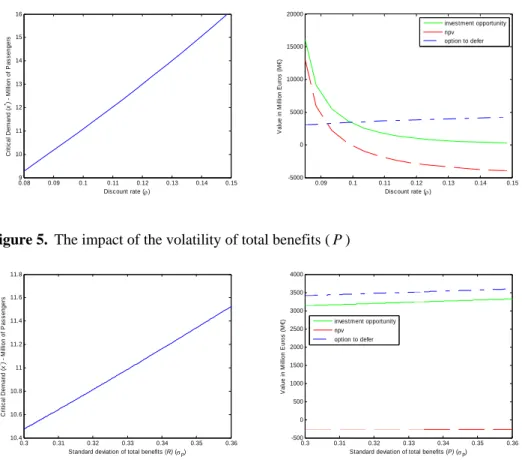
Figure 4. The impact of the discount rate

0.089 0.09 0.1 0.11 0.12 0.13 0.14 0.15 10 11 12 13 14 15 16 Discount rate (ρ) C rit ic a l D e m a n d ( x *) - M illion of P a s s enger s 0.09 0.1 0.11 0.12 0.13 0.14 0.15 -5000 0 5000 10000 15000 20000 Discount rate (ρ) V a lu e in M illio n E u ro s ( M € ) investment opportunity npv option to defer

Figure 5. The impact of the volatility of total benefits ( P )

0.3 0.31 0.32 0.33 0.34 0.35 0.36 10.4 10.6 10.8 11 11.2 11.4 11.6 11.8

Standard deviation of total benefits (R) (σP)

C rit ic a l D e m a n d ( x *) - M illion of P a s s enger s 0.3 0.31 0.32 0.33 0.34 0.35 0.36 -500 0 500 1000 1500 2000 2500 3000 3500 4000

Standard deviation of total benefits (P) (σP)

V a lu e in M illio n E u ro s ( M € ) investment opportunity npv option to defer

Taking into account increases in the volatility of total benefits (Figure 5) and/or in the volatility of the investment’s expenditures (Figure 6), delays are more and more

superior, given the increase induced in the critical demand level. Considering a constant NPV towards variations in the standard deviation of the total benefits (Figure 5) or in the standard deviation of investment’s expenditures (Figure 6) and a value of the option to defer changing directly with these two uncertainty factors, the investment’s opportunity value increases when uncertainty increases. This is an expected behaviour according to the literature about investments’ valuation under uncertainty.

Figure 6. The impact of the volatility of the investment expenditures

0 0.02 0.04 0.06 0.08 0.1 0.12 0.14 0.16 0.18 0.2 9.8 10 10.2 10.4 10.6 10.8 11

Standard deviation of investment expenditures (σγ)

C rit ic a l D e m a n d ( x *) - M ill io n of P a s s enger s 0 0.02 0.04 0.06 0.08 0.1 0.12 0.14 0.16 0.18 0.2 3000 3500 4000 4500 5000 5500 6000 6500 7000 7500 8000

Standard deviation of investment expenditures (σγ)

V a lue i n M il li on E u ro s ( M €) investment opportunity npv option to defer

Figure 7. The impact of the volatility of the number of passengers

0 0.05 0.1 0.15 0.2 0.25 8.5 9 9.5 10 10.5 11 11.5 12 12.5 Standard deviation of x (σx) C rit ic a l D e m a n d ( x *) - M illion of P a s s enger s 0 0.05 0.1 0.15 0.2 0.25 -4000 -2000 0 2000 4000 6000 8000 10000 12000 14000 Standard deviation of x (σx) V a lu e in M illio n E u ro s ( M € ) investment opportunity npv option to defer

Major operating speed of the HSR service entails a major reduction in the travel time value, given by

0 2 0 η η η −

, which in turn, implies diminishment on the critical demand level from which is optimal to implement the investment (Figure 9). In result of the major benefits afforded by the project, the NPV registers an increase slightly superior to the increase occurred in the value of the investment opportunity. Therefore, there is a propensity for the anticipation of the decision of implementing the investment, with the option to defer loosing value.

Figure 8. The impact of the time-to-build 0 1 2 3 4 5 6 7 8 9 10 10.5 10.6 10.7 10.8 10.9 11 11.1 11.2 11.3 11.4 11.5 Years of construction (n) Cr it ic a l Dem and ( x *) - M ill ion of P a s s enger s 0 1 2 3 4 5 6 7 8 9 10 -1000 -500 0 500 1000 1500 2000 2500 3000 3500 4000 Years of construction (n) V a lue i n M il li on E u ro s ( M €) investment opportunity npv option to defer

Figure 9. The impact of the reduction in the value of travel time

50 55 60 65 70 75 80 9.4 9.6 9.8 10 10.2 10.4 10.6 10.8 11

Reduction of value of travel time (η) - in %

Cr it ic al Dem a nd ( x *) - M illio n o f P a s s e n g e rs 50 55 60 65 70 75 80 3000 4000 5000 6000 7000 8000 9000

Reduction of value of travel time (η) - in %

V a lue i n M il li on E u ro s ( M €) investment opportunity npv option to defer

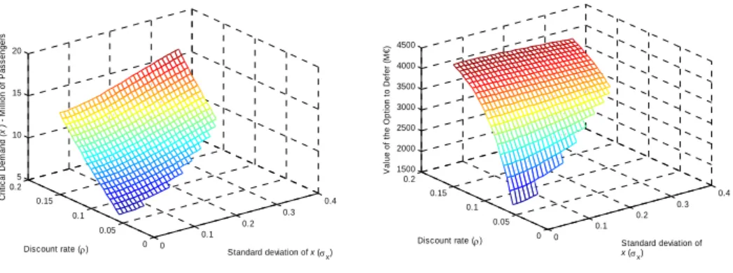
Figure 10. The impact of both the volatility of the number of passengers and

the discount rate

0 0.1 0.2 0.3 0.4 0 0.05 0.1 0.15 0.2 5 10 15 20 Standard deviation of x (σx) Discount rate (ρ) C ri ti c al Dem and (x *) - M illio n o f P a s s e n g e rs 0 0.1 0.2 0.3 0.4 0 0.05 0.1 0.15 0.2 1500 2000 2500 3000 3500 4000 4500 Standard deviation of x (σx) Discount rate (ρ) V a lu e of t he O p ti on t o Def e r ( M € )

In this scenario, the behaviour of the valuation results regarding the discount rate variations (Figure 4), demand volatility (Figure 7), time-to-build (Figure 8) and reduction in the value of travel time (Figure 9) turns out to be as expected, maintaining

similar to the behaviour registered even when only one uncertainty factor is considered (Pimentel et al. 2006). Potential differences occurs on the level of the valuation results,

except the value of the option to defer which maintains in similar levels to the scenario with only one uncertainty factor.

Similar to the behaviour of Pimentel’s et al. (2006) model with only one stochastic

variable, the critical demand level presents a direct relation with the discount rate and with the demand standard deviation (Figure 10). The value of the option to defer shows a major sensibility to the discount rate compared to the demand volatility. The sensibility of the option to defer regarding the demand standard deviation has a direct relation for lower values of discount rate. Nevertheless, for superior values of discount rate, this relation changes, becoming an inverse relation, as we may observe on the upper side of the graphic on the right side of Figure 10.

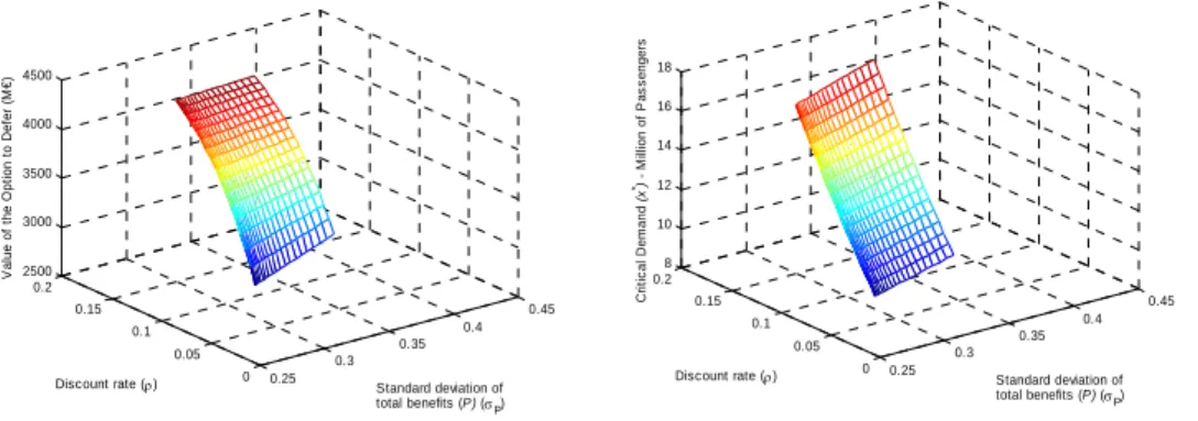
As for the joint impact of the discount rate and standard deviation of total benefits on the critical demand level and on the value of the option to defer (Figure 11), the only significant difference registered regarding Figure 10 is the direct relation between the uncertainty factor related to total benefits and the value of the option to defer which maintains in the whole interval considered for the discount rate. However, this direct relation tends to smooth as the discount rate increases. This delay of the inversion in the relation between the uncertainty factor and the value of the option to defer is due to the increase of the weight of uncertainty in the model, induced by the introduction of more factors, comparatively to the weight of other parameters, like for instance the discount rate.

Figure 11. The impact of both the volatility of the total benefits and the discount rate

0.25 0.3 0.35 0.4 0.45 0 0.05 0.1 0.15 0.2 2500 3000 3500 4000 4500 Standard deviation of total benefits (P) (σP) Discount rate (ρ) V a lu e of t he O p ti on t o Def e r ( M € ) 0.25 0.3 0.35 0.4 0.45 0 0.05 0.1 0.15 0.2 8 10 12 14 16 18 Standard deviation of total benefits (P) (σP) Discount rate (ρ) C rit ic a l D e m a n d (x *) - M illion of P a s s enger s

Figure 12. The impact of both the growth rate and the volatility of the investment expenditures 0 0.05 0.1 0.15 0.2 0 0.02 0.04 0.06 7 8 9 10 11 12 Standard deviation of investment expenditures (σγ) Growth rate of investment expenditures (µγ) Cr it ic al Dem a n d (x *) - M illi o n of P a s s enge rs 0 0.05 0.1 0.15 0.2 0 0.01 0.02 0.03 0.04 0.05 2600 2800 3000 3200 3400 3600 Standard deviation of investment expenditures (σγ) Growth rate of investment expenditures (µγ) V a lu e of t he O p ti on t o Def e r ( M € )

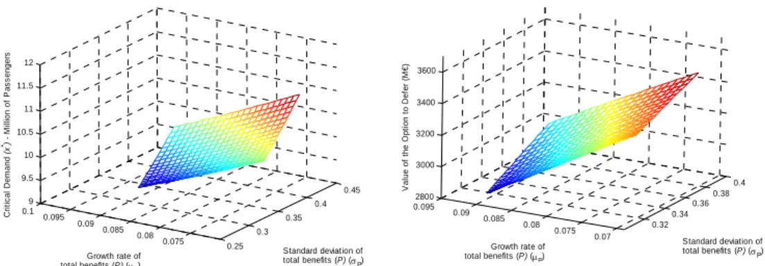
Figure 13. The impact of both the growth rate and the volatility of the total benefits

0.25 0.3 0.35 0.4 0.45 0.075 0.08 0.085 0.09 0.095 0.1 9 9.5 10 10.5 11 11.5 12 Standard deviation of total benefits (P) (σ_P) Growth rate of total benefits (P) (µP) Cr it ic al Dem and (x *) - M illi o n of P a s s enger s 0.32 0.34 0.36 0.38 0.4 0.07 0.075 0.08 0.085 0.09 0.095 2800 3000 3200 3400 3600 Standard deviation of total benefits (P) (σ_P) Growth rate of total benefits (P) (µ_P) V a lu e of t h e O p ti on t o Def e r ( M €)

The impact of both the growth rate and volatility upon the critical demand level and the value of the option to defer, considering three uncertainty factors, may be observed in Figure 12 for the investment’s expenditures and in Figure 13 for total benefits. Whenever it’s expected a superior growth on the value of the investment’s expenditures and/or on the growth rate of total benefits, not only the critical demand level diminishes, leading to the anticipation of the project’s implementation, but also the option to defer looses value.

On the other hand, higher values, either of the standard deviation of the investment’s expenditures or of the standard deviation of total benefits, leads to appreciations on the value of the option to defer and on the critical demand level, triggering major delays in the investments implementation.

This behaviour towards uncertainty may also be observed in Figure 14, which highlights the influence of project’s total uncertainty on the critical demand level and on the value of the option to defer.

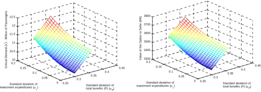
Figure 14. The impact of both the volatility of the investment expenditures and the

volatility of the total benefits

0.25 0.3 0.35 0.4 0.45 0 0.05 0.1 0.15 0.2 10 10.5 11 11.5 12 12.5 Standard deviation of total benefits (P) (σP) Standard deviation of investment expenditures (σγ) Cr it ic al D e m a nd (x *) M ill io n of P a s s enge rs 0.25 0.3 0.35 0.4 0.45 0 0.05 0.1 0.15 0.2 3300 3400 3500 3600 3700 3800 Standard deviation of total benefits (P) (σP) Standard deviation of investment expenditures (σ_γ) V a lu e of t he O p ti on t o Def e r ( M €)

Figure 15. Critical demand level sensibility for variations on each one of the three

uncertainty sources 0 0.05 0.1 0.15 0.2 0.25 8.5 9 9.5 10 10.5 11 11.5 12 12.5

Standard deviation of x (σx) and x (σγ)

C rit ic a l D e m a n d ( x *) - M il li o n of P a s s e nger s sensibility to σ_x sensibility to σγ sensibility to σ_R

In general, among the three uncertainty factors, the one regarding demand appears to be the most sensitive in the valuation results, as we may see in Figure 15. The critical demand level presents a similar sensibility regarding the uncertainties on the investment’s expenditures and on the benefits per user.

The inclusion of two more uncertainty factors, besides the one related with demand, although not changing significantly the valuation results, turns the valuation model more complete, assuring a major accuracy in the decision making. This behaviour may be justified since the model demonstrates that the existence of a positive growth rate

upon the investments’ expenditures allied to its uncertainty cause a contrary impact to the one resultant from the uncertainty inclusion upon the benefits per user.

5. Conclusion

The present paper develops a ROA model to value the HSR investment’s opportunity and the optimal timing to invest, regarding several uncertainty effects. This model relies on the utility function equilibrium between the HSR service and the conventional railway service for its users.

The option to defer with multiple uncertainty factors is subject to a deeper analysis. The decision to invest instead of delay is obtained regarding the uncertainty that surrounds the demand level for the new HSR service, the investment’s expenditures and the benefits resultant from the project. Although the demand variable represents the main uncertainty factor (Rose, 1998), the developed model can simultaneously measure the impact of the other two uncertainty variables in the optimal investment decision. This last two uncertainty variables show an opposite impact in the valuation process.

The net effect of including uncertainty in the model, regarding the investment’s expenditure and the benefits, shall depend on the magnitude of the according individual effects. If throughout time it’s expected an appreciation on the investment’s expenditure amount, the option to defer shall loose value, ceteris paribus. The inclusion of

uncertainty upon the benefits shall increase the value of the option to defer, resultant from a major exposure of the project to uncertainty.

In the future we intend to apply the model to the new Portuguese HSR project, using real data1. This application should provide the necessary feedback to guide additional improvements in the structure of the modelling framework. We also aim to include demand shocks on the valuation framework, considering different probability distribution functions.

1

Portuguese public authorities have shown availability to release, to the authors, data regarding the new Portuguese rail link.