A comparative study of tree-based models for churn prediction : a case study in the telecommunication sector

i

A COMPARATIVE STUDY OF TREE-BASED

MODELS FOR CHURN PREDICTION: A CASE

STUDY IN THE TELECOMMUNICATION SECTOR

Ibrahem Hamdy Abdelhamid Kandel

name

Dissertation presented as partial requirement for obtaining

the Master’s degree in Statistics and Information

ii

A COMPARATIVE STUDY OF TREE-BASED

MODELS FOR CHURN PREDICTION: A CASE

STUDY IN THE TELECOMMUNICATION SECTOR

Ibrahem Hamdy Abdelhamid Kandel

Dissertation presented as partial requirement for obtaining

the Master’s degree in Statistics and Information

i

Title: A COMPARATIVE STUDY OF TREE-BASED MODELS FOR CHURN PREDICTION: A CASE STUDY IN THE

TELECOMMUNICATION SECTOR

Subtitle:

Student

full name Ibrahem Kandel

MEGI

201

8

201

8

Title: A COMPARATIVE STUDY OF TREE-BASED MODELS FOR CHURN PREDICTION: A CASE STUDY IN THE

Subtitle:

Student

ii

NOVA Information Management School

Instituto Superior de Estatística e Gestão de Informação

Universidade Nova de Lisboa

A COMPARATIVE STUDY OF TREE-BASED MODELS FOR CHURN

PREDICTION: A CASE STUDY IN THE TELECOMMUNICATION

SECTOR

by

Ibrahem Hamdy Abdelhamid Kandel

Dissertation presented as partial requirement for obtaining the Master’s degree in Information Management, with a specialization in Market Research and CRM

Advisor: Professor Roberto Henriques

iii

ACKNOWLEDGEMENTS

I would like to express gratitude towards my master’s thesis advisor, Professor Roberto Henriques, for providing guidance on my thesis.

iv

ABSTRACT

In the recent years the topic of customer churn gains an increasing importance, which is the phenomena of the customers abandoning the company to another in the future. Customer churn plays an important role especially in the more saturated industries like telecommunication industry. Since the existing customers are very valuable and the acquisition cost of new customers is very high nowadays. The companies want to know which of their customers and when are they going to churn to another provider, so that measures can be taken to retain the customers who are at risk of churning. Such measures could be in the form of incentives to the churners, but the downside is the wrong classification of a churners will cost the company a lot, especially when incentives are given to some non-churner customers. The common challenge to predict customer churn will be how to pre-process the data and which algorithm to choose, especially when the dataset is heterogeneous which is very common for telecommunication companies’ datasets. The presented thesis aims at predicting customer churn for telecommunication sector using different decision tree algorithms and its ensemble models.

KEYWORDS

Churn prediction; Predictive modelling; Decision trees; Data mining; Customer churn; CRM; Random Forests; Decision Trees; Ensemble; Bagging

v

INDEX

1.

Introduction ... 1

2.

Literature review ... 3

2.1.

Churn Prediction ... 3

2.2.

KDD cup 2009 ... 5

2.3.

Missing values literature review ... 7

2.4.

Decision tree literature review ... 9

2.4.1.

THAID (Messenger & Mandell, 1972) ... 10

2.4.2.

ID3 (J R Quinlan, 1986): ... 10

2.4.3.

C4.5 (J Ross Quinlan, 1993): ... 10

2.4.4.

CART (Breiman et al., 1984): ... 11

2.4.5.

CHAID (Kass, 1980): ... 12

2.4.6.

FACT (Loh & Vanichsetakul, 1988): ... 12

2.4.7.

QUEST (Loh & Shih, 1997): ... 12

2.4.8.

CRUISE (H. Kim & Loh, 2001): ... 12

2.4.9.

CTREE (Hothorn, Hornik, & Zeileis, 2006): ... 13

3.

Methodology ... 14

3.1.

Dataset ... 14

3.2.

Data pre-process ... 15

3.2.1.

Categorical features handling ... 16

3.2.2.

Imputing Missing Values ... 16

3.2.3.

Feature Selection ... 17

3.2.4.

Treating imbalance ... 17

3.3.

Decision tree ensembles ... 19

3.3.1.

Bootstrap aggregation (Bagging) & Random Forests ... 20

3.3.2.

Boosting ... 21

3.3.3.

Stacked Ensembles ... 23

3.4.

Resampling techniques... 24

3.4.1.

Leave-One-Out- Cross-Validation ... 24

3.4.2.

K-Fold Cross-Validation ... 25

3.5.

Evaluation and Hyperparameter Optimization ... 25

3.5.1.

Model Evaluation using AUC of the ROC curve ... 25

3.5.2.

Hyperparameter Optimization ... 27

vi

3.7.

H2O platform ... 28

4.

RESULTS ... 29

4.1.

Preprocess results ... 29

4.1.1.

Imputing Missing Values for the three datasets ... 29

4.1.2.

Balancing the datasets ... 30

4.1.3.

Feature Selection ... 31

4.2.

Final model auc results ... 32

4.3.

Analysis of the results ... 32

4.4.

Key Findings ... 33

5.

Conclusion and FUTURE WORK ... 34

vii

LIST OF ABBREVIATIONS AND ACRONYMS

CCP

Customer Churn Prediction

CRM

Customer Relationship Management

Decision trees

RF

Random Forests

GBM Gradient Boosting Machine SVM

Support vector machines

MCAR Missing completely at random KNN K-nearest neighbor algorithm

SMOTE Synthetic Minority Oversampling Technique SGBT Stochastic Gradient Boost Trees

AdaBoost Adaptive Boosting PCA Principal component analysis MI Mutual Information

LMT Logistic Model Trees OOB Out of bag

AUC Area Under the ROC Curve ROC Receiver operating characteristic

KDD Knowledge discovery in databases

viii

LIST OF FIGURES

Fig.1.1 Customer Churn Model ……… 1

Fig.2.1 Results of paper (Azeem et al., 2017) ……… 4

Fig.2.2 Voting classifier ………….………..6

Fig.2.3 Missing values Imputation Methods ………8

Fig. 2.4 Models used in Churn Prediction ………9

Fig.3.1 CRISP-DM model ………..………..14

Fig.3.2 The Flowchart of the Preprocess Step ………..………..15

Fig.3.3 Missing values distribution………16

Fig.3.4. Different Approaches to treat Imbalance ……….18

Fig.3.5. Bias-Variance VS. Model complexity ………..19

Fig.3.6. Bagging Algorithm Flowchart ………..20

Fig.3.7. AdaBoost ………..22

Fig.3.8. Stacking Ensemble ………24

Fig.3.9.ROC curve ………….………..26

Fig.3.10. The Flowchart of the proposed model ………28

ix

LIST OF TABLES

Table 1 Summary of Decision trees algorithms ………. 13

Table 2 Confusion matrix………26

Table 3 The AUC results for Churn Dataset Missing Value Imputation ………..………29

Table 4 The AUC results for Appetency Missing Value Imputation ………..29

Table 5 The AUC results for Up-Selling Missing Value Imputation ………30

Table 6 The AUC results for Churn Dataset Balancing ………30

Table 7 The AUC results for Appetency Dataset Balancing ……….………30

Table 8 The AUC results for Up-Selling Dataset Balancing ………..………31

Table 9 The AUC results for Churn Dataset after Feature Selection ……….………31

Table 10 The AUC results for Appetency Dataset after Feature Selection ………31

Table 11 The AUC results for Up-Selling Dataset after Feature Selection………32

Table 12 The AUC results of the Final model……….32

Table 13 The KDD 2009 winners ………...33

LIST OF ALGORITHMS

Algorithm 2 C4.5 Root Choice for Discrete Features Algorithm ……….… 11

Algorithm 3 C4.5 Root Choice for Numeric Features Algorithm ……….… 11

Algorithm 4 Feature selection using Random Forest Algorithm ……….… 17

Algorithm 5 Random Forest Algorithm……….…21

Algorithm 6 AdaBoost.M1 Algorithm……….…23

1

1. INTRODUCTION

In today’s business, a lot of advertising and offers appears everywhere in television, internet and billboards which puts the customer in a lot of offers like free subscription or discounts, so many customers change their service providers to get the benefit of these offers. The term churn is now well known in today’s businesses, customer churn is the scenario where the customer loses interest in continuing his business in the company and seeks another company to fulfill his needs, this can have a huge impact on the profits of the company (Buckinx & Van Den Poel, 2005). Right now, it’s one of the most important topics in saturated business, especially in the rapidly growing telecommunication sector, knowing that the cost of acquiring new customers is as high as ten times to retain the existing customers (Lu & Ph, 2002), mainly due to fierce competition between telecommunication companies. It's very important to the companies to reduce the revenue loss due to the leaving customers, the reasons for churn differs from company to another and from customer to another. Mainly there are two types of churners: the involuntary churners “forced to leave” and the voluntary churners, the involuntary churners happens when the company decide to end the contract due to many reasons like the case when they don’t satisfy their part of agreement between them and the company, while the voluntary churners is the type that most of the researches are done on, because these customers are mainly the most profitable customers and the company wants to retain them as their customers. The reasons for voluntary churns differs a lot from one customer to another, mainly in telecommunication it’s due to higher cost, quality, lack of features, privacy issues and others (Sharma & Sachdeva, 2017).

The Customer churn prediction can be defined as assigning a probability to leave the company next to each customer in the company dataset, to make it viable to the firm to indicate which customer has the highest propensity to churn, then for the company to set a threshold to indicate which probability to churn they want to tackle, then the customers clusters whom crossed this threshold will be targeted by a specially designed marketing plan to increase their retention. Different approaches was introduced to increase customer retention (Fig.1), while targeting all of the churners clusters will be Monterey exhausting, that’s why the companies must select wisely which of these customers to target, instead of targeting every one also known as uplift modeling (Coussement, Lessmann, & Verstraeten, 2017).

Fig.1.1 Customer Churn Model

The steps of the process will be: using predictive modeling to detect which customer has the highest probability to churn, then by using uplifting modeling to detect which customers can be targeted with the retention plan. The customer churn topic is discussed many times in telecommunication sector (Mahajan, Misra, & Mahajan, 2015), many kinds of research were done to know what are the optimization algorithms to use to expect when the customers are going to churn before they do, knowing that about 30 percent of the customers are going to churn per year (Lu & Ph, 2002). To acquire a new customer, the company is going to

2 spend ten times more than to retain the already existing customers, so by now to retain the existing customers is more profitable than acquiring new customers (Lu & Ph, 2002). By the help of the recent techniques in data mining, companies succeed in having insights about their customer behavior either by using the usual Sociodemographic variables or by using more advanced variables like their customer call center data (Hadden, Tiwari, Roy, & Ruta, 2006).

There are many machine learning techniques being adopted in Customer churn like Logistic regression, Decision trees, Artificial neural networks and Support vector machines (Hadden, Tiwari, Roy, & Ruta, 2007; Mahajan, Misra, & Mahajan, 2015). Now in the era of big data a lot of researchers try to draw the light on the importance of inclusion of the customer data from the social platforms to be included in the customer behavior analysis (Bi, Cai, Liu, & Li, 2016; Liu & Zhuang, 2015; Singh & Singh, 2017). Because datasets of the companies are usually containing redundant values, missing values among others which decreases any model predictive power, that's where the data preprocess is vital in the process of building any model. The challenges that must be treated before implementing the model is imbalance problem, missing values, curse of dimensionality and others The imbalance problem can be defined as having one class outnumbered the other class, in the case of customer churn its usually that the non-churner customers’ numbers are much higher than the churner customer (Burez & Van den Poel, 2009), which will have a huge influence on most of machine learning algorithms. The challenge of having degenerative features which are features with zero variance, meaning that there is no change in the values of that features, which makes it useless in the prediction model also it will create a numerical difficulty.

The occurrences of missing data in any dataset brings a huge impact on the performance of any machine learning algorithm, many algorithms had been used to tackle the challenge of missing values (Noh, Kwak, & Han, 2004), but still the uncertainty of these values will result in low predictive power of the model because of the bias created by the new values. The curse of dimensionality can be treated by using a proper feature reduction techniques, which mainly falls into three categories: filter methods, wrapper methods and embedded methods (Raza & Qamar, 2017). Identify the true churner from the retained customer is crucial, because of the high cost of retaining a non-churner customer, which consider resource wasting so the issue of the model accuracy is very important (Khan, Jamwal, & Sepehri, 2010), to assess the quality of the model can be detected by using the AUC of the ROC curve (Vuk, 2006), which is commonly used in the classification problems.

The model proposed in this thesis is decision tree-based models, the importance of using decision tree models is that they are fast to compute and highly interpretable. Which have a great advantage for companies to not only estimate the propensity of each customer to churn, but also to understand which features are important to retain the customers in the future, also it has a great advantage over many machine learning algorithms, which the decision trees can deal with heterogeneous data, defined as data that contain numerical and categorical features. In this paper, the used dataset is the KDD Cup 2009 small dataset (Guyon, Lemaire, Vogel, et al., 2009), which was provided by the French telecommunication company Orange for predicting three binary classifications: churn, upselling and cross-selling. The main objective of this thesis is to evaluate and analyze of performance of tree-based models to predict the churn probability of customers for telecommunication sector, the proposed machine learning models are decision trees, Random forest and Gradient Boost Machine. The results will be assessed by using AUC of the ROC curve as proposed by the evaluating committee of the challenge.

The remainder of the paper is organized as follows: in section 2 discussion about the literature review made on papers presented using the KDD 2009 dataset. In section 3 the data pre-process step. In section 4 the models proposed in the study. In section 5 the results of each model. In section 6 Conclusions. In section 7 future studies.

3

2. LITERATURE REVIEW

The classification task of customer churn has been studied in different sectors where its applicable like: banking sector (Ali & Arıtürk, 2014; Mohanty & Naga Ratna Sree, 2018; Şen & Bayazıt, 2015), insurance companies (Morik & Köpcke, 2004; R. Zhang, Li, Tan, & Mo, 2017; W. Zhang, Mo, Li, Huang, & Tian, 2016) online social networks (Ngonmang, Viennet, & Tchuente, 2012; Oentaryo, Lim, Lo, Zhu, & Prasetyo, 2012; Óskarsdóttir et al., 2016), Churn in online gaming (Borbora & Srivastava, 2012; Castro & Tsuzuki, 2015; Liao, Chen, Liu, & Chiu, 2015) and telecommunication sector which is the task of this paper. The literature review section will be divided into two parts: The first part is a brief overview of previous studies about customer churn in telecommunication sector and the second part is a brief overview of previous studies done on KDD 2009 dataset.

2.1.

C

P

In the study done by Pendharkar (2009) the author proposed two genetic-algorithm based on neural network to predict customer churn for telecommunication sector, to their knowledge that was the first paper to implement genetic algorithm to predict churn for telecommunication sector. They used a real-world dataset with 195,956 customers and four variables then They split the dataset into 70% for training and 30% for testing. The first genetic algorithm was used for prediction and the second was used to increase the performance of the first one. They compared the performance of their algorithm to a statistical z-score model using many evaluating criterions including ROC curve. Their findings were that the medium sized neural networks with number of hidden layers equal to twice the number of variables performed better than the statistical z-score model, but it was more computationally expensive than the statistical model.

In the study done by Owczarczuk (2010) the author tested some supervised machine learning algorithm to predict churn for prepaid clients of a Polish telecommunication company. The real-world dataset they used had 1381 variables and 85,274 customers. The author compared interpretable models like logistic regression, Fisher linear discriminant analysis and decision Trees. The author selected 50 variables based on Student’s t-test. The author main findings were that logistic regression outperformed other algorithms that the author used, and he stated that decision trees were very unstable for the dataset he used. Also, the author argues that the usage of ensemble models is improper to predict customer churn for telecommunication sector. In the study done by Azeem, Usman, & Fong (2017) the authors used fuzzy classifiers algorithm to predict customer churn for telecommunication sector. They used a real-world dataset from South Asian telecommunication company that had 722 variables and 600,000 customers. To their knowledge that was the first paper to implement fuzzy classification algorithm to predict churn for telecommunication sector. Feature selection was based on domain knowledge, and the authors chose the most important 84 variables. they used 80% of the dataset for training and the reminder 20% to test the model. The dataset contained only numeric features, they used min-max algorithm to normalize all the dataset to be in the range of 0-1. The authors Used oversampling technique to balance the dataset since, it had only 9% churners and the percentage after the balancing was 60% non-churners and 40% churners. They used AUC of the ROC curved to evaluate the model. They compared the performance of some fuzzy classifier namely, FuzzyNN, VQNN, OWANN and FuzzyRoughNN with other non-fuzzy algorithms: neural network, logistic regression, decision tree C4.5, Support vector machine, Adaboost, Gradient boost machine and Random Forests. Their main findings were: that fuzzy classifiers are more accurate than other classifiers to predict customer churn. The worst performing classifier was the C4.5 decision tree, then the ensemble algorithms achieved an average AUC 0f 0.5725, the best classifier was OWANN (Fuzzy-rough ownership) with AUC of 0.68.

4 Fig.2.1. Results of paper (Azeem et al., 2017)

In paper by authors Effendy, Adiwijaya, & Baizal (2014), the authors worked on an Indonesian telecommunication dataset which has only 0.7% churners, their objective was to tackle the problem of imbalance in their dataset by combining both SMOTE (Chawla, Bowyer, Hall, & Kegelmeyer, 2002) to the minority class and undersampling algorithm to majority class. By using only the weighted random forest it didn’t improve the accuracy of the model so they included the SMOTE algorithm for the minority class and simple under sampling for the majority class to balance the dataset. They removed any feature with more than 80% of missing value, also redundant features were remove as well. Also, they converted all the categorical features into numeric. To validate the model, they used K-Fold validation with 10 folds. They compared the performance of the model without treating the imbalance to the models with under sampling and over sampling. By combining over sampling with under sampling it increased the model performance significantly rather than using the weighted random forest without balancing the dataset. Weighted Random Forest was introduced because the random forest algorithm is biased towards the majority class (Chen, Liaw, & Breiman, 2004), a penalty can be added on misclassifying the minority class. By adding weights to each class, the majority class has less misclassification cost than the minority class. The weights adjustment is done in two phases: the induction phase and the terminal phase. Weighted majority vote is used to determine the predicted class of each data point. By aggregating the weighted vote of each tree to get the final predicted class. Out-of-bag can be used to tune the weights used.

In the study done by Hassouna, Tarhini, Elyas, & Abou Trab (2015) the authors made a comparison between logistic regression and decision trees using a real-world dataset provided by an English mobile operator. They used two balanced datasets (50% Churners): one for training the algorithm with 17 variables and 19,919 customers and another dataset for testing with 17 variables and 15,519 customers. CART, C5.0 and CHAID decision trees were used to be compared to logistic regression. They used AUC of the ROC curve, top-decile and overall accuracy to evaluate and compare between different models. Their main findings were that the C5.0 decision tree outperformed other algorithms including Logistic regression with AUC of 0.763. Their findings contradicted with the findings of the author (Owczarczuk, 2010) where he stated that logistic regression is more accurate to predict customer churn for telecommunication sector.

In the study done by Jayaswal, Prasad, & Agarwal (2016) the authors compared between C5.0 decision tree and two main decision trees ensembles: Random Forests and Gradient Boosting Machine to predict customer churn for telecommunication sector using a publicly available dataset. The dataset had 21 variables and 3333 customers with 15% churners, the authors followed the findings of (Burez & Van den Poel, 2009) which stated that sampling techniques will not affect the performance of the models used and so they didn’t treated the imbalance in the dataset. They used 75% of the dataset for training and 25% for testing. Their main findings were that: The GBM outperformed the Random Forest and C5.0 for this dataset.

In paper by authors Amin et al. (2017) the authors explored rough set approach (Pawlak, 1982) to the churn problem, which outperformed other machine learning algorithms for their used dataset.They split the dataset into 70% for training and 30% for validation. They compared the rough set approach to the state of the art algorithms used in churn prediction like ANN, DT and SVM. They noted that for this dataset the rough set approach achieved better accuracy than all other compared algorithms.

5 In paper by authors Kamalraj & Malathi (2013), the authors studied the performance and accuracy of C4.5 (J Ross Quinlan, 1993) and C5.0 decision trees. The study was done on a public dataset with 3333 customer. C5.0 decision tree achieved higher accuracy with better performance in regards to computational power.

2.2. KDD

2009

In paper by authors Lo et al. (2009), the authors combined the three classification task (churn, appetency and up sell) into one joint Multi-class classification task. Three ensemble techniques were used to classify this multi-class classification task: The first technique the authors used was L1-regularized maximum entropy because of its robustness against outliers but its main drawback is that it cannot deal with missing values because this model will assume no missing data, so the authors added a binary feature next to each feature with missing value to indicate that this feature had missing value, then all the categorical features were hot-encoded which resulted in 111,670 additional features to the dataset, and to scale the dataset the authors used Log and linear scaling. The second technique: a heterogeneous base learner was introduced to handle the numeric and categorical features which was a tree classifier “decision stump” then coupling the base learner with Adaboost algorithm to increase the predictive performance of the base learner. Finally, the third ensemble was a selective Naive Bayes classifier that automatically treat the categorical features with high cardinality by grouping them also, the NB classifier will discretize the numerical features. Then the authors applied a post processing algorithm “SVM” to adjust the predictive power across the three classification tasks, because for some data points the classifier will assign higher probabilities to more than one label. Overfitting was avoided using K-fold cross validation to better train the classifiers. The authors ranked the third place with AUC of 0.8461 for the slow track competition (15,000 features and 50,000 instances).

In paper by authors Xie & Coggeshall (2009), the authors used Stochastic gradient boosting tree as a classifier to predict the three class labels for the large and small datasets. The authors bagged 5 gradient boosted decision trees using different seeds and then took the average votes of these trees models to increase the model performance. The authors chosen the log-likelihood as a loss function for the stochastic gradient boosting tree. To preprocess the dataset, the authors binned high cardinality categorical features “greater than 1000 unique levels” into 100 new levels. Also, the authors discretized 10 numerical features that had small unique values. For imputing missing values, the authors imputed the categorical features with a risk factor and imputed numerical features with adding another feature that contain an identification to identify these features as having missing values. The authors removed redundant features with very low variance also removed quasi-constant features. Also, SGBT algorithm was used for feature selection as a wrapper method. To treat the imbalance in the dataset down sampling was used to down sampled the majority class label. The authors split the dataset into 75% for training and 25% for testing the algorithm. Then the authors used 5-fold validation for the training dataset. The authors tried logistic regression algorithm, but it scored lower than the SGBT. Also, SVM was tried that had an approximate score as SGBT but with more computational time. The authors ranked the second in the fast track with large dataset (AUC = 0.8448) and third place in the slow track for the large dataset (AUC = 0.8478) and scored an AUC of 0.8478 for the small dataset.

In paper by authors Kurucz et al. (2009), the authors worked on the large dataset which contain 15,000 features and 50,000 instances. The authors tried different feature reduction algorithms including: distance, information and dependence measures but these algorithms didn’t perform well as they tended to over fit the data by selecting non-predictive features or selecting highly correlated features and so these measures can decrease the generalizability of the model. The feature selection algorithm the authors opted for was the LogitBoost due to its robustness against outliers. The final classifier the authors opted was LogitBoost combined with ADTrees by taking their average classification. The algorithms the authors opted scored AUC of 0.8457.

6 In paper by authors Niculescu-Mizil et al. (2009), the authors worked on the large dataset considered categorical missing values as a separate value, and imputed the numeric features using the mean of the feature. Also, an additional indicator feature was added to indicate that this feature had a missing value. The authors hot-encoded the top 10 common values of each categorical feature to make all the dataset to be numeric, afterwards the authors standardize the dataset, then all the redundant features were removed from the dataset. The authors used 10-fold validation technique to validate their results on the training dataset. The authors built a library of base classifiers: RF, Boosted trees, LR, SVM, DT, NB, KNN and Regularized Least Squares Regression. Some classifiers were trained on reduced datasets using PCA, Pearson correlation and MI. The authors noted that the best individual classifier on Churn label was Boosted trees followed by LR then RF. The highest AUC obtained by using only the base classifiers was 0.7354 for churn label. The authors used an ensemble selection algorithm with greedy forward stepwise selection to select an ensemble from the library of base classifiers which yielded an AUC of 0.7563 for churn label. The AUC of churn increased to 0.7629 after adding new features generated from tree induction and co-clustering. The final AUC of Churn was 0.7651 and the average AUC overall labels was 0.8519.

In paper by author Yabas (2013), the author used the small dataset which contains 230 features and 50,000 instances. For the preprocess step the authors removed all the redundant features and any feature with more than 99% missing values. The authors imputed the numerical missing values with the mean of the features and imputed the categorical features with by placing a value “Missing”. The authors normalized the numerical features to be in the range 0 and 1. To handle the high cardinality of the categorical features the authors kept only the top 10 most frequent levels and grouped the rest of levels into a level called “others”. The authors trained 250 models with 20 algorithms. The authors tried NN, AdaBoost and SVM but pointed out these models are very computationally expensive and reported that their results are very poor compared to other algorithms they used and so the authors eliminated these models from there analysis. The base model algorithms proposed by the authors included an ensemble of C4.5 decision trees, logistic regression, bagging and random forests. The authors pointed out that the RF was the best performing base classifier. The authors argued that each classifier they used needs a specific preprocessing step and so the authors built a specific preprocessing step for each classifier which will construct a meta-classifier and then all the meta-classifiers with AUC greater than or equal 0.69 will vote for every instance and the majority of these votes will predict the label of each test instance. The meta-classifiers that exceeded the threshold AUC were LR, DT with Bagging, RF. The final AUC achieved was 0.7230 across all the three labels (churn, appetency and up-selling).

Fig.2.2. Voting classifier (Yabas, 2013)

In paper by authors Doetsch et al. (2009), the authors used small dataset, they reformulated the task as having multi-task approach where they trained a single classifier with three binary outputs instead of single classification task, which yielded an increase of 0.015 to the AUC. They used Information Gain ratio as a feature selection algorithm and likelihood-ratio test as a ranking algorithm, then they tried MLP, SVM, LMT and boosted decision stumps. The best-performing technique was by stacking the output of boosted decision stumps algorithm as a level 0 algorithm then using logistic model tree with AUC splitting criteria as level 1. The

7 algorithm used to implement the boosted decision stumps is the AdaBoost.MH algorithm and for LMT they implemented their own modification which was a C4.5 tree where each node estimates a LogitBoost model. In paper by authors Miller et al. (2009), the authors used large dataset, the missing values for the numerical and categorical features were treated as a separate level, used decision trees and boosting, in their attempt to treat the high cardinality categorical features, they tried to aggregate levels with less than 1,000 observations into 20 levels based on their response, but that created the problem of overfitting, so to prevent this problem they tried to aggregate the features independent of their responses instead they aggregated based on their observations, by creating four groups being the first group includes the features that had 1000 observations, and the second group is the levels that has 500 to 999 observations, and the third group are levels with 250-499 observations, and the forth are levels that had 1-250 levels, which prevented the overfitting problem and increased the AUC by 0.0015 compared to the single-level aggregation.

2.3. M

One of the most challenging obstacles in machine learning is imputing missing values, where Imputation of missing values is the treatment to the problem of missing data by replacing it with values (Batista & Monard, 2003), to obtain a complete data set with no missing values. Firstly, the missing data mechanism should be known cause depending on the mechanism a proper method should be implied, where missing data mechanism describes the process that determines each data points likelihood of being missing, there are three main categories (Enders, 2010):

1- MCAR: Missing completely at random, can be thought like random missing values where the missing values is unrelated to the dataset, the probability of having missing values in any feature doesn’t depend either on it or other variables in the dataset. Can be verified by using a complete feature in the dataset by comparing the mean of the observed data points by the mean of the missing data points and the two means shouldn’t be different.

2- MAR: Missing at random, the probability of having missing values in any feature in the dataset doesn't depend on its value, but instead it depends on other features in the dataset. Cannot be verified unless the values of missing features are known.

3- MNAR: Missing not at random, the probability of having missing values in any feature in the data set depends on the values of the feature itself, cannot be verified unless the values of missing features are known.

Deletion methods:

- Listwise deletion: only the observed values are retained and the rest is removed from the analysis(Schafer, 1999), but its main disadvantage that it can result in biased results (Graham, 2009) also it will remove a lot of useful information from the dataset, only accepted for 5% missing values. - Pairwise deletion: used when estimating covariance or correlation matrices, for each pair it will use

the complete cases for both.

Single imputation methods: single value of each missing data point, its main disadvantage is that one single value cannot rightly predict the missing value and if there’s not only one value is enough for this missing value (Rubin, 1988)

- Mean imputation: Impute the missing values with the mean of the available data points of the same feature, produces unbiased estimates of the variance.

- Regression imputation: Impute the missing values using regression to predict the missing values using other features as predictors.

- Stochastic regression imputation: Impute the missing values using regression but it will add a stochastic value to the predictions of the regression imputations, produces an unbiased estimate with MAR datasets.

8 - Hot deck imputation: the data are clustered into several cluster then the missing value will be imputed with the mean or the mode of the cluster it falls in, prediction models where the creation of a machine learning model to estimate the missing value using other features in the dataset.

- Baseline observation carried forward BOCF: Impute the missing values by taking the baseline observation as a replacement for the missing data.

- Last observation carried forward LOCF: Impute the missing values by taking the last observed value as a replacement for the missing data.

- Strawman imputation: The numerical missing values will be substituted by the median, while the categorical missing values will be substituted by the most frequent level, has a great advantage of being rapid, for NMAR missing values the strawman imputation technique can have higher accuracy for highly missing values more than 75% (Shah, Bartlett, Carpenter, Nicholas, & Hemingway, 2014). Multiple imputation methods: By having multivariate complex dataset an adequate missing data method is needed, multiple imputation (Rubin, 1987, 1996) is commonly used to predict missing values in complex datasets where many features has missing values. Where it Creates several data sets with different values of each missing data point, it will take into account the uncertainty of each missing value meaning that not only one value can rightly predict the missing value (Azur, Stuart, Frangakis, & Leaf, 2011). Two major methods to impute missing values using multiple imputation are: joint modeling (JM) and the fully conditional specification (FCS) method, where the joint modeling method is based on normality and linearity of all features and the imputations will be generated by linear regression, and so the JM is only suited for continuous features. While Fully conditional specification does not assume normality or linearity of the features of the study and so it can be used either for continuous or categorical features.

Under assumption that the missing values in this dataset is MAR, multiple imputation technique can be used like: MICE which is a multiple imputation technique (van Buuren & Oudshoorn, 2011) based on the method of fully conditional specifications which has the basic assumption that the missing values are missing at random, meaning that their probability of being missing depends only on the observed data (Azur et al., 2011). The imputation method depends on the nature of variable distribution, whether its continuous or binary the used algorithm will be linear regression or logistic regression respectively (Azur et al., 2011). Fig.3.4. summarize different techniques to impute missing values.

9

2.4. D

By looking at the next figure by the authors García, Nebot, & Vellido (2017) which states that DT is the most used model in the recent Churn prediction literature, due to its interpretability and ease of deployment, also because of its hierarchical shape which can present to decision makers as a set of rules. Decision trees recursively partition the data space and fit a simple prediction rule within each partition, starting at the root of the tree to classify a new data point then follows the branch indicated by the result of the decision rule, until a leaf node is reached, the class of the leaf node is the class of the new data point.

Fig.2.4. Models used in Churn Prediction (García et al., 2017)

Two main categories of decision trees can be found in literature: classification trees and regression trees (Rokach & Maimom, 2014), where the classification trees are the designed for categorical target feature and its prediction power can be measured using misclassification cost, the regression trees are designed for continuous target feature and its prediction power can be measured using square difference between the observed and predicted values. The used dataset has a binary output, so the used algorithm will be classification decision tree.

Classification decision trees produces rectangular disjoints sets of the dataset, by recursively partitioning the dataset one feature each time (Loh, 2011). A decision tree structure consists of either a leaf node or a decision node, where the leaf node contains the predicted class and the decision node contain a decision rule to further split the data (Miroslav Kubat, 2015). To split the data a splitting criterion is used, where a single or multiple feature can be used, the single splitting criterion named univariate split and the multiple features named multivariate split (C. E. Brodley & Utgoff, 1995), univariate decision trees are more common because of its simplicity and comprehensibility (Murthy, 1996) but its main drawback that it will only divide the space with a boundary that is orthogonal to the feature being used (C. Brodley & Utgoff, 1992).

There are many types of decision trees proposed in literature named THAID (Messenger & Mandell, 1972), ID3 (J R Quinlan, 1986), C4.5 (J Ross Quinlan, 1993), CART (Breiman, Friedman, Stone, & Olshen, 1984), CHAID (Kass, 1980), FACT (Loh & Vanichsetakul, 1988), CRUISE (H. Kim & Loh, 2001), QUEST (Loh & Shih, 1997) and CTREE (Hothorn, Hornik, & Zeileis, 2006). To better understand their use, commonly used decision tree algorithm will be explained in this section.

- If 𝑃1, … , 𝑃𝐾is a fraction of record belonging to the 𝐾different classes in a node 𝑁:

1-Then the Gini-index 𝐺(𝑁) of the node 𝑁 is defined as: 𝐺(𝑁) = 1 − ∑𝐾𝑖=1𝑃𝑖2,where the value of 𝐺(𝑁) lies

between 0 and (1 −1

𝐾), the smaller the value of 𝐺(𝑁) the greater the skew, If the classes are evenly balanced

the value is (1 −1

10 2- The entropy 𝐸(𝑁) of the node 𝑁 is defined as: 𝐸(𝑁) = − ∑𝐾𝑖=1𝑃𝑖. log 𝑃𝑖, where the value of the entropy

lies between 0 and log 𝐾, when the records are perfectly balanced among different classes the value of entropy is log 𝐾 which is the maximum entropy while the smaller the entropy the greater the skew in the data. The Gini-index and entropy provide an effective way to evaluate the quality of a node in terms of its level of discrimination between the different classes.

Given a N labeled training set {(xi, yi)} for , and the target variable “Churn or Not”

Entropy and Information gain

Entropy for two classes classification: by having S set of examples and is the proportion in the class , and is the proportion in the class , knowing that

The generalization of Entropy for i target classes, so by having S set of instances and P_i is the fraction of S set that has output value of i

the change in the Entropy can be measured by Information Gain (Hssina, Merbouha, Ezzikouri, & Erritali, 2014)

2.4.1. THAID (Messenger & Mandell, 1972)

The first published classification tree algorithm was Theta Automatic Interaction Detection THAID which splits a node by exhaustively searching overall 𝑋 and 𝑆 for the split that minimizes the total impurity of its two child nodes.

2.4.2. ID3 (J R Quinlan, 1986):

ID3 decision tree was designed for nominal features only, continuous data have to be converted into nominal features using binning or other embedding methods before it can be used. Uses information gain as splitting criterion, Usually doesn’t guarantee an optimal solution, cause it will got stuck in local minima due to its greedy partition strategy. Doesn’t apply any pruning strategy so it has high risk of overfitting the data.

2.4.3. C4.5 (J Ross Quinlan, 1993):

C4.5 decision tree was an evolution of ID3 (J R Quinlan, 1986) uses entropy for its impurity function called gain ratio, multiway split yields a binary split if the selected variable is numerical; if it is categorical, the node is split into 𝐶 subnodes, where 𝐶 is the number of categorical values. Can handle numeric attributes by splitting the attribute’s value range into two subsets. Specifically, it searches for the best threshold that maximize the gain ratio criterion. All values above the threshold constitute the first subset and all other values constitute the second subset. Uses a pruning procedure which removes branches that do not contribute to the accuracy and replace them with leaf nodes. Can split a node into more than two children nodes, their number depending on the characteristics of the X variable. Uses Pessimistic Error Pruning. Require that the target attribute will have only discrete values

11 Algo.1. C4.5 Decision Tree Algorithm

Algo.2. C4.5 Root Choice for Discrete Features

Algo.3. C4.5 Root Choice for Numeric Features

2.4.4. CART (Breiman et al., 1984):

CART decision tree algorithm uses Gini-index (Light & Margolin, 1971) as a splitting criterion. It first grows an

overly large tree and then prune it to a smaller size using 10-fold cross-validation Cost Complexity Pruning to minimize an estimate of the misclassification error. Minimal Cost-complexity pruning: The basic idea of cost-complexity pruning is to calculate a cost function for each internal node meaning that all nodes that are neither leaves nor roots in the decision tree.

The cost function is given by:

𝑅𝛼(𝑇) = 𝑅(𝑇) + 𝛼 . |𝐿𝑒𝑎𝑣𝑒𝑠(𝑇)|

Where

𝑅(𝑇) = ∑𝑡∈𝐿𝑒𝑎𝑣𝑒𝑠(𝑇)𝑟(𝑡) . 𝑝(𝑡) = ∑𝑡∈𝐿𝑒𝑎𝑣𝑒𝑠(𝑇)𝑅(𝑇)

𝑅(𝑇) the misclassification cost of the sub-tree obtained after pruning of a certain branch. C4.5 Decision Tree Algorithm:

Let X be the training set: grow (𝑇)

1. Find the feature 𝑥 that contribute the most information about the class labels.

2. Divide 𝑇into subsets of 𝑇𝑖, each must have different values at 𝑥

3. For each 𝑇𝑖:

If all examples in 𝑇𝑖 belongs to the same class, then create a leaf labeled

with this class, otherwise, apply the same process recursively to each training subset: Grow (𝑇𝑖)

Decision Tree root choice from discrete features C4.5 Algorithm:

1. Calculate the entropy of training set T using the probabilities 𝑃𝑝𝑜𝑠 of the

positive labeled class and 𝑃𝑛𝑒𝑔 of the negatively labeled class

𝐻(𝑇) = −𝑃𝑝𝑜𝑠log2𝑃𝑝𝑜𝑠− 𝑃𝑛𝑒𝑔log2𝑃𝑛𝑒𝑔

2. For each attribute 𝑥 that divides 𝑇 into subsets 𝑇𝑖 with related sizes 𝑃𝑖:

3. Calculate the entropy of each subset 𝑇𝑖

4. Calculate the average entropy: 𝐻(𝑇, 𝑥) = ∑ 𝑃𝑖 𝑖. 𝐻(𝑇𝑖)

5. Calculate the information gain: 𝐼(𝑇, 𝑥) = 𝐻(𝑇) − 𝐻(𝑇, 𝑥) 6. Choose the feature with the highest value of information gain.

Decision Tree root choice from numeric features C4.5 Algorithm: 7. For each numeric feature 𝑥𝑖:

8. Sort the training example by values of 𝑥𝑖

9. Find the candidate threshold 𝜃𝑖𝑗 as those lying between data points of

different labels

10. For each 𝜃𝑖𝑗 determine the amount of information contributed by the

Boolean feature thus created

12 𝛼 the cost complexity parameter for that branch, for each value of 𝛼 there is a unique smallest tree that minimizes the cost complexity measure 𝑅𝛼(𝑇).

Gradually increasing the complexity parameter 𝛼 starting from 0, will lead to a nested sequence of trees decreasing in size. The optimal tree size is determined by 10-fold cross validation, the data set is divided into 𝑁 = 10 subsets, one of the subsets is used as independent test set while the other 𝑁 − 1 subsets are used as training test, the tree growing and pruning procedure is repeated N times, each time with a different subset as test set. For each tree the misclassification error is calculated, the tree with the lowest misclassification error is the optimal tree. Breiman proposed the 1 𝑆. 𝐸. rule which will select the smallest tree whose cost complexity measure is within 1 standard error of the cost complexity for the tree with the minimum misclassification error. CART is implemented in the R system(Team, 2009) as RPART (Therneau & Atkinson, 1997).

2.4.5. CHAID (Kass, 1980):

CHAID decision tree uses P-value with a Bonferroni correction as a splitting criterion. Has an advantage of splitting the node into more than two children nodes. Usually doesn't prune the result tree. According to Wei-Yin (2014) the major drawback of using the greedy search approach in CART and C4.5 decision trees is its selection bias. Selection bias usually happens when the variables with high cardinality will have a high chance to be selected to split nodes more than the low cardinality variables. For the decision tree to be unbiased all the variables must have the same chance to be selected given that all the features are independent of the target feature.

Unbiased variable selection Decision Trees: As being proposed by FACT decision tree (Loh & Vanichsetakul, 1988) CRUISE, GUIDE and QUEST decision trees use splitting criteria based on two-steps. The first step, each feature is tested for association with the target feature and then the most significant feature is selected to split based on it. The second step, an exhaustive search over all the dataset is performed, and because every feature has an equal chance to be selected if and only if each feature is independent of the target feature. So that approach is unbiased.

2.4.6. FACT (Loh & Vanichsetakul, 1988):

In FACT decision tree the splits at each node will depend on the number of the classes in each variable. If any categorical features appeared in the dataset it will be transformed into dummy variables (H. Kim & Loh, 2001). For FACT to have univariate splits, the features will be ranked using F-test of ANOVA then linear discriminant analysis will be applied to the top features to split the nodes based on it. The tree size will be determined by ANOVA test (H. Kim & Loh, 2001).

2.4.7. QUEST (Loh & Shih, 1997):

In QUEST decision tree it will split the features into two categories: Ordered and Unordered features, then it will run ANOVA test on the ordered features and Chi-Square test on the unordered features and so the selection bias will be eliminated. QUEST Supports univariate and linear combination splits. As in CART (Breiman et al., 1984) it uses ten-fold cross-validation to prune the trees.

2.4.8. CRUISE (H. Kim & Loh, 2001):

CRUISE decision tree was an improvement of QUEST (Loh & Shih, 1997). Splits each node of the tree into multiple children nodes depending on the number of classes of the target variable. It avoids the selection bias by using two statistical tests: Chi-Square test and F-Test at each node to select which feature to split based on. Uses the same pruning method as CART (Breiman et al., 1984).

13

2.4.9. CTREE (Hothorn, Hornik, & Zeileis, 2006):

CTREE decision tree was introduced to avoid selection bias CTREE uses permutation tests where it uses p-values from permutation distributions of influence function-based statistics to select split variables. Does not use pruning; it uses stopping rules based on multiplicity adjusted p-values to determine tree size. The algorithm is implemented in the R package PARTY.

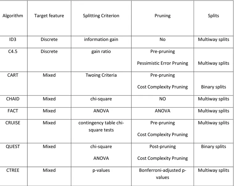
In the following table, different DT are summarized based on their target function, splitting criterion, pruning and splits techniques.

Algorithm Target feature Splitting Criterion Pruning Splits

ID3 Discrete information gain No Multiway splits

C4.5 Discrete gain ratio Pre-pruning

Pessimistic Error Pruning Multiway splits

CART Mixed Twoing Criteria Pre-pruning

Cost Complexity Pruning Binary splits

CHAID Mixed chi-square NO Multiway splits

FACT Mixed ANOVA ANOVA Multiway splits

CRUISE Mixed contingency table

chi-square tests

Pre-pruning Cost Complexity Pruning

Multiway splits

QUEST Mixed chi-square

ANOVA

Post-pruning Cost Complexity Pruning

Binary splits

CTREE Mixed p-values Bonferroni-adjusted

p-values

Multiway splits

14

3. METHODOLOGY

To conduct a data mining project a systematic process should be followed. Mainly two process had introduced (Olson & Delen, 2008): The CRISP-DM (Wirth & Hipp, 2000) Cross Industry Standard Process for Data Mining process which is widely used by a lot of data mining practitioners (Olson & Delen, 2008) and the SEMMA process Sample, Explore, Modify, Model, Asses. As being pointed out by the authors of Azevedo & Filipe Santos (2008) CRISP-DM can be more comprehensive than the SEMMA model, and so it will be followed in this research.

The CRISP model consists of six stages Fig.3.1., the first step is the business understanding: which is about understanding the business objectives and needs, and to develop a project plan with time frame of when the whole data mining project will take, and a time frame for each stage. The Second stage is the data preparation step: Start with data collection, data visualization, data summary and to discover insights from the data, then to check the data quality. The third step is the Data preparation: Also known as data preprocessing phase, where the final dataset will be constructed from the initial dataset. The forth step is the modelling stage: various machine learning algorithms are applied, and their parameters are tuned to suit the dataset understudy. The fifth step is the Evaluation stage: the models obtained from the previous step are evaluated and their accuracy and performance are assessed, frequently will be reverted to previous step for better choosing different model. The sixth step is the deployment stage: the final stage where the model built will be deployed to be used by the user, usually in a form of an API.

Fig.3.1. (Wirth & Hipp, 2000) CRISP-DM model

3.1. D

The dataset being used in this paper is a real-world dataset provided by the French telecommunication company Orange to develop three Customer Relationship Management algorithms to improve the company marketing strategies (Guyon, Lemaire, Vogel, et al., 2009):

1- Customer Churn: A binary feature which can be defined as probability that the customers will leave the company voluntary to another for better offer or other reasons as stated in the introduction. 2- Customer appetency: A binary feature which can be defined as Probability that the customer will buy

a new product from the company

3- Customer up-sell: A binary feature which can be defined as Probability that the customer will upgrade his original plan to another one.

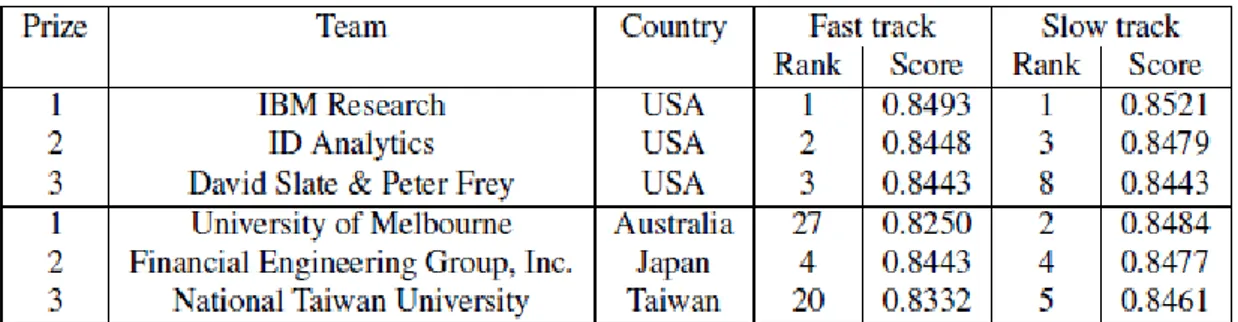
15 The dataset was released as a part of the 15th edition of Knowledge Discovery and Data Mining (KDD) annual competition, which is hold annually to explore new algorithms and to enrich the scientific community. In 2009 the French telecommunication company Orange released a challenge to detect these labels. The challenge had two paths: The fast path and a slower one, for the fast path the contestants had to submit their result in five days and for the slow path the contestants had one month to submit their results. Two datasets were released: large dataset which contains 15,000 features (14,770 numerical features and 260 Categorical features) and 100,000 instances, 50,000 to train the dataset and 50,000 to test the algorithms and a small dataset which contains 230 features (190 numerical features and 40 Categorical features) and 50,000 instances to train the dataset and another 50,000 to test the algorithms. Submissions were evaluated using AUC of the ROC curve, with the average AUC of the three class labels were used to rank the contestants. All the features presented in the large and in the small datasets were anonymized for the customer privacy and no meta-information was provided to explain any of the features. Table 1 shows the winners of this competition for the large and the small datasets.

KDD 2009 dataset was chosen because of its availability and its suitability for data mining techniques because the dataset had many challenging tasks from being multi-class classification task also, the dataset contains missing values that needed to be imputed and so many imputation algorithms can be experimented using this dataset, the dataset is high dimensional and so many feature selection techniques can be studied and examined on this dataset. The dataset used in this paper is the small dataset for the sake of computational resources available. The dataset is heterogeneous meaning that it contains numerical and categorical features. Also, the dataset is high imbalanced meaning that the number of positive instances is much lesser than the negative instances, for churn the number of positive instances is only 3764 out of 50,000 and for appetency only 764 out of 50,000 and for up-sell only 1400 out of 50,000. All the results reported here are the AUC of the ROC curve of the small dataset of the KDD 2009 challenge.

3.2. D

-

Dealing with high dimensionality dataset is very challenging for machine learning algorithms and before applying any algorithm a proper preprocess is required (Kumar & Sonajharia, 2014). According to the authors Han & Kamber (2000) The preprocessing step is vital for building the model, which can be used to remove noisy and redundant data to improve the model performance and accuracy.

Fig.3.2. The Flowchart of the Preprocess Step

Prior to using the dataset in data mining models high cardinality categorical features should be handled, treat incomplete data, treat imbalance in the data if found and to remove empty features and impute missing values if found. Especially for classification tasks the number of features used must be minimum, if the dimensionality is large this will increase the computation cost also it will produce error and decrease the performance of the used algorithms (Ertel, Black, & Mast, 2017). By having one feature with above average values compared to the other features, it will overpower the rest of the features by doing any analysis, to overcome this issue the usage of normalization is preferable to maintain the balance in the data, even many software packages will do it by default, to treat this a linear scaling will be used meaning to scale the numerical features to range of [0,1]. Models that are built on smooth functions such as regression models, are affected greatly by different scales in that dataset (Casari & Zheng, 2018). While, tree-based models that are based on splitting technique are robust against different scales in that dataset (Casari & Zheng, 2018). The used models in this research are tree-based models, so no scaling will be performed.

16

3.2.1.

By having a high cardinality categorical feature in the data set will not only decrease the accuracy of the model, it will also increase the computational time needed. High cardinality can be defined as non-ordered fields having large number of unique values can reach up to thousands or even millions (Micci-Barreca, 2001). Under the assumption that any feature with more than 500 unique level is only text with no predictive power, these features will be removed from the modeling process. Any levels with less than 5% prevalence will be combined into a new group called “Others”. Var217 has 13990 levels, means that each level has less than 1% prevalence in the dataset, also Var214 which has 15415 levels and the highest level appeared 74 times in the dataset with prevalence of 1.5%. Also, Var192 and Var204 has many levels with less than 1% of each level so both will be removed from the analysis. As being proposed by (Miller et al., 2009) the attempt to resolve this issue will be by creating four groups of levels based on the number of observations, where levels with more than 1000 observations will be grouped together, levels with exposure between 500-999 will be grouped together, levels with exposure between 250-499 levels will be grouped together, levels with exposure between 1-250 will be grouped together.

3.2.2.

By using R Library(healthcareai) we can see the count of missing values in each variable, the following table have the percentage of missing values with respect to each variable.

Fig.3.3. Missing values distribution

In practice one important parameter for MICE imputation method is the number of datasets to create to impute the missing value, the factors affecting this decision are: The size of the dataset, the amount of missing values and computational resources available, for the dataset in hand imputing 10 datasets with 5 imputations seemed feasible. Before running the MICE algorithm, all the empty and variables with more than 50% missing value were removed from the analysis under the assumption that these variables cannot be used. By removing all the totally empty features, then to remove any variable with more than 50% missing value, 77 variables will

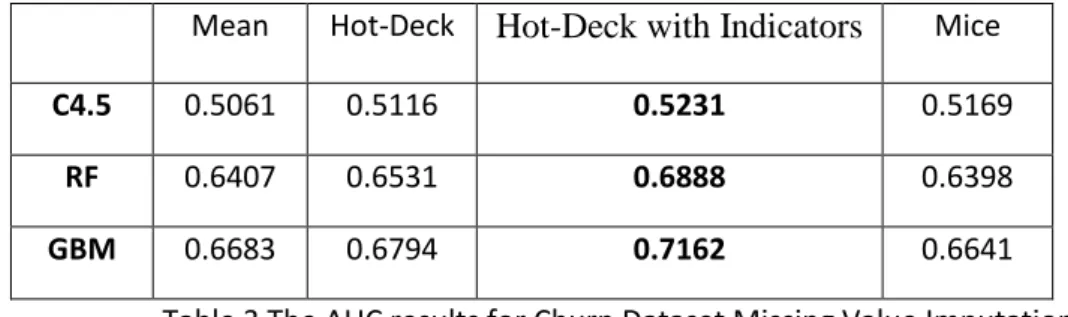
17 be retained for building the model. For MICE the features with the least amount of missing values will be imputed first, then used in subsequent imputations, then the next feature with the second least amount of missing values will be imputed then used with the first in subsequent imputations. Missing values will be imputed using mice, hot-deck and mean then their accuracy will be assessed using AUC of the ROC to choose the best method to impute the missing values.

3.2.3.

As being introduced in Bellman (1961) the curse of dimensionality can be defined as having too many

dimension in the dataset that will make the classifier takes a lot of time also it will decrease its

predictive power. The cornerstone of data preparation for any type of algorithm is choosing which

feature to use and to exclude any redundant features that could increase computational power and

reduce the prediction power (Kalousis, Prados, & Hilario, 2007). Also, using feature selection reduce

the overfitting of the model, and thus increasing the stability of the model (Kumar & Sonajharia,

2014). According to the authors Wu, Qi, & Wang (2009) feature selection has two main approaches

which are filter methods and wrapper methods based on the relationship between the features and

the algorithm in use.

Filter methods: no feedback from the used algorithm, evaluation is being done by using feature

selection criterion like information gain, distance measure, dependency or consistency, but its main

drawback that it requires an exhaustive search over all the dataset which in case of

telecommunication can contains hundreds of features. While, wrapper methods use feedback from

the used algorithm where the prediction power of the model is used as the main criteria of selecting

which feature to be used. In this thesis the wrapper method using Random Forests (Breiman, 2001)

will be chosen because the variable selection and supervised machine learning will be optimized

together as a complete learning system (Svetnik, Liaw, & Tong, 2004). The main idea of the algorithm

is that it is based on iteratively removing the lowest ranking features, then to assess the model AUC

using K-Fold Cross Validation. As being suggested by Determan (2015) the same algorithm can be

repeated using Gradient boosting machine (Friedman, 2001). The AUC result of the random forest

algorithm and the Gradient Boosting machine are reported in the results section and the best

performing algorithm will be used to select the most important features.

Algo.4. Feature Selection using Random Forest Algorithm

3.2.4.

The Imbalance problem is very common in the field of machine learning (YANG & WU, 2006), because usually the desired label is not well represented in the dataset. The imbalance in the dataset in some cases can be very high which can reach up to 10,000,000 times i.e. the majority class is higher than the minority class by 10,000,000 times (J. Wu, Brubaker, Mullin, & Rehg, 2008). The case in telecommunication sector is the churners

Feature Selection using Random Forest Algorithm (Svetnik, Liaw, & Tong, 2004): 1- Using K-Fold validation to split the dataset into training and validation

sets.

2- Using all the features of the training dataset to train the random forest algorithm.

3- Record the rank of every feature according to their importance. 4- Half of the least important features will be removed.

5- Train another random forest on the rest of the features.

6- Record the rank of the rest of features according to their importance. 7- Half of the least important features will be removed.

8- Steps 2-7 will be repeated from 10 to 50 times. 9- Select the top ranked features.

18 percentage is most likely to be the minority class. There are a lot of studies on methods and algorithms on how to treat dataset unbalance mainly the algorithms presented in the paper from Batista, Prati, & Monard (2004), the authors presented a comparative study of ten popular imbalance handling techniques which can be summarized into two main groups: random and non-random techniques, random techniques are non-heuristic techniques which include under-sampling and over-sampling techniques, where random under-sampling is to remove data points randomly from the majority class to balance the dataset. Random over-sampling is to replicate the minority data points randomly to balance the dataset but empirical studies showed that over-sampling tends to overfit the data (Prati, Batista, & Monard, 2008).

A lot of Non-random techniques was introduced mainly to put some heuristics in selecting which data point to remove instead of doing it randomly. A few examples of undersampling non-random techniques includes Tomek links (Tomek, 1976) which is an undersampling technique where data points belonging to the majority class are the data points to be removed from the model. Formally Tomek Link can be defined as: by having two classes in the dataset ‘+’ and ‘-’, assume two data points each belongs to different class: 𝑥𝑖, 𝑥𝑗 and the distance

between them is 𝑑(𝑥𝑖, 𝑥𝑗) then 𝑥𝑖 and 𝑥𝑗 are Tomek link if for any data point 𝑥𝑙, 𝑑( 𝑥𝑖, 𝑥𝑗) < 𝑑( 𝑥𝑖, 𝑥𝑙) 𝑜𝑟 𝑑( 𝑥𝑖, 𝑥𝑗) <

𝑑( 𝑥𝑗, 𝑥𝑙), in a summary for any two data points if they are Tomek Link then either one of them are noise or both

of the data points located on the boundary between ‘+’ and ‘-’.

Another non-random undersampling algorithm is One-sided selection (M Kubat & Matwin, 2000) which can be defined as: by having a subset 𝑆 which is selected randomly from population 𝑇 where each data point in 𝑇 has an equal probability to be chosen. The OSS algorithm reduces the population space 𝑇 by removing the majority class examples and so it will create a new population 𝑂 = 𝑇 − 𝐶 where 𝐶 is the minority class data points. Then a subset 𝐴 is selected from 𝑇 where 𝐴 will correctly classify 𝑇 by using 𝐾𝑁𝑁 = 1. Then noisy and border line data points will be removed from 𝑂. The OSS algorithm is showed in Algo.2.

One of the most widespread non-random oversampling technique was introduced by Chawla, Bowyer, Hall, & Kegelmeyer (2002) called SMOTE , which stands for Synthetic Minority Oversampling Technique. Instead of replicating the minority data points SMOTE produces new synthetic minority data points using the feature space, based on weighted average of the K-NN. SMOTE has three hyper parameters that need to be tuned in first: 1- The over sampling percentage needed to create new data points for the minority class. These new data points won't be replicate of the already exist data points but instead, it will be generated using KNN to reduce overfitting (Up & In, 2017). 2- The under-sampling percentage needed to delete some majority data points. 3- KNN used to impute the synthetic data points. (Chawla et al., 2002) used KNN=5 in their analysis. The AUC result of the OSS, Tomek Links and SMOTE are reported in the results section. Different approaches to treat Imbalance can be found in Fig.3.11.