Essays on Dynamic Macroeconomics and Risk Attitudes.

(1)

Essays on Dynamic Macroeconomics and

Risk Attitudes

by

Rui Leite

Doctoral Thesis in Economics

Supervised by Alper C¸ enesiz

(2)

(3)

Biographical note

I was born in 1981, in the city of Porto, Portugal, where I later completed my undergraduate education in Economics at the School of Economics and Management of the University of Porto. I began my professional career in 2006, working as a Research Assistant for Professor Nuno Sousa Pereira at the Research Centre in Industrial, Labour and Managerial Economics (CETE). I have also worked as an Economist at the Portuguese Ministry of Finance and at the Portuguese Healthcare Regulation Authority, and since 2009 I collaborate as a Researcher on the South African Panel Study of Small Business and Health, a research project coordinated by Professor Li-Wei Chao. I currently work as an Economist at the Portuguese Public Finance Council.

(4)

Acknowledgements

I am deeply grateful to my supervisor, Alper C¸ enesiz. From him I have learned much about Economics, and this doctoral thesis would not be possible without his thoughtful guidance and support.

Helena Szrek, Li-Wei Chao, and Nuno Sousa Pereira o↵ered constant encouragement and wise advice throughout my PhD. I was fortunate to work with them on di↵erent research projects over the years, learning immensely in the process. For all this I express my deepest gratitude.

I thank Ana Paula Ribeiro and Anabela Carneiro for their comments and suggestions on early drafts of the material I present in this thesis. The final versions of the essays have benefited greatly from their input.

My time at the School of Economics and Management of the University of Porto was enriched by the interactions I had with many of its faculty members. I owe a special recognition to Álvaro Aguiar, Aurora Teixeira, Inês Drumond, José Varejão, Manuel Mota Freitas, Óscar Afonso, and Paulo Vasconcelos.

Finally, I thank my family and specially my wife, Ana, for their love and support.

(5)

Abstract

This thesis is a collection of three essays in Economics. The first essay concerns the di↵erence in the business cycle volatility of the unemployment rates of high-skill and low-skill workers. I show that from the late 1990s onwards the business cycle volatility of the unemployment rate has been higher for high-skill workers in the United States and thirteen European Union countries. I address this volatility gap with a business cycle model in which firms value skill diversity, each worker supplies a specific variety of skill, and households pay a cost to search and find new jobs. I calibrate the model to United States data and show it can successfully replicate the observed unemployment volatility gap, as well as generate unemployment rates that are substantially more volatile than output.

The second paper modifies a standard two-country international business cycle model to allow for a state-dependent risk aversion parameter, and investigates whether key mismatches between the theory and the data can be explained by varying risk aversion. I show that even though the dynamics of the exchange rate are linked with the behavior of the risk aversion parameter, under a reasonable calibration the volatility of the exchange rate is largely una↵ected by how strongly countercyclical risk aversion is. In contrast, I find that the correlation between the movements in the exchange rate and the movements in the consumption ratio is substantially reduced in the presence of countercyclical risk aversion. I show that these results hold under di↵erent assumptions about the behavior of the risk aversion parameter, and under di↵erent assumptions about the household’s preferences over the consumption-leisure bundle.

The third essay investigates the relationship between risk taking propensity and economic and health expectations using data from a longitudinal survey conducted in the Tshwane Municipality, South Africa. I find evidence that economic expectations significantly predict risk taking propensity, with better expectations being associated with higher willingness to take risks. The results hold with two di↵erent measurement scales for risk attitudes, and hold under a variety of robustness checks. I find some evidence that health expectations predict risk taking propensity, but the robustness checks fail to confirm the results. The findings highlight a channel through which economic expectations can a↵ect decision making under risk, and I discuss its potential implications for entrepreneurial activity and our understanding of asset bubbles.

(6)

Resumo

A presente tese reúne três ensaios na área cient´ıfica da Economia. O primeiro ensaio relaciona-se com a temática da volatilidade das taxas de desemprego dos trabalhadores qualificados e não qualificados. Apresenta-se evidência emp´ırica de que, a partir do final dos anos 90, a volatilidade da taxa de desemprego nos Estados Unidos e em treze pa´ıses europeus é superior para os trabalhadores qualificados. Este diferencial de volatilidade é analisado no âmbito de um modelo de ciclos de negócios reais em que as empresas valorizam a diversidade de qualifica¸cões, cada trabalhador oferece uma qualifica¸cão única e as fam´ılias suportam os custos de procura de novos empregos. Uma calibra¸cão do modelo para os Estados Unidos replica o diferencial de volatilidade observado nos dados, bem como a maior volatilidade da taxa de desemprego face ao produto.

O segundo ensaio apresenta uma extensão do modelo de ciclos de negócios internacionais com duas economias, a qual contempla fam´ılias com aversão ao risco variável, investigando-se o efeito desta modifica¸cão sobre discrepâncias existentes entre o modelo e os dados. Os resultados demonstram que embora a dinâmica da taxa de câmbio esteja relacionada com a aversão ao risco, uma calibra¸cão plaus´ıvel deste modelo não modifica substancialmente a volatilidade da taxa de câmbio face ao modelo padrão, mantendo-se esta substancialmente abaixo do que é observado nos dados. Em contraste, os resultados demonstram que a correla¸cão entre os movimentos da taxa de câmbio e os movimentos do rácio do consumo é menor na presen¸ca de aversão ao risco contra-c´ıclica, reduzindo substancialmente o diferencial entre o modelo e os dados. A análise de robustez mostra que estes resultados se verificam com diferentes especifica¸cões para as preferências das fam´ılias e para o comportamento do parâmetro de aversão ao risco.

O terceiro ensaio investiga a rela¸cão entre a aversão ao risco e as expectativas que os indiv´ıduos formam sobre a economia e sobre o seu próprio estado de saúde, usando para o efeito dados longitudinais provenientes de um inquérito realizado no munic´ıpio de Tshwane, na África do Sul. Apresenta-se evidência de que as expectativas económicas constituem um previsor estatisticamente significativo da aversão ao risco, estando melhores expectativas associadas a uma menor aversão ao risco. Estes resultados verificam-se em duas escalas usadas para medir a aversão ao risco e são confirmados por uma variedade de testes de robustez. A evidência sugere que as expectativas sobre o próprio estado de saúde podem constituir um previsor da aversão ao risco, mas este resultado não é confirmado sob diferentes testes de robustez. Este ensaio real¸ca um canal através do qual as expectativas económicas podem influenciar a tomada de decisão em contexto de risco, discutindo-se também as suas potenciais implica¸cões para a actividade empreendedora e para a forma¸cão de bolhas especulativas.

(7)

List of Figures

2.1 Cyclical volatility of the unemployment rate in the United States, 40-quarters-ahead, by skill group . . . 8 2.2 Response of selected model variables to an exogenous technology shock 22 3.1 E↵ects of countercyclical risk aversion under di↵erent response lags . 61 3.2 Risk aversion movements – benchmark model vs. asymmetric response 63 4.1 Coefficient estimates and 95% confidence intervals for the economic

and health expectation variables, under di↵erent values of ⇢. . . 93

(11)

List of Tables

2.1 Cyclical volatility of the unemployment rate in the United States and

thirteen E.U. countries, by skill group . . . 6

2.2 Cyclical volatility of the unemployment rate in the United States, by skill group . . . 7

2.3 Baseline calibration . . . 18

2.4 Standard deviations, autocorrelations and cross correlations with output, from model simulations and U.S. data, 1976:Q1–2016:Q4 . . . 20

2.5 Standard deviations, autocorrelations and cross correlations with output, from model simulations and U.S. data, sub-period analysis . . 26

2.6 Standard deviations, autocorrelations and cross correlations with output, from model simulations and U.S. data, sub-sample analysis . 29 2.7 Sensitivity analysis for simulations of the U.S. data, 1976:Q1–2016:Q4 32 3.1 Baseline parameter calibration . . . 50

3.2 Exchange rate statistics . . . 52

3.3 Business cycle statistics . . . 53

3.4 The role of the elasticity of intertemporal substitution . . . 58

3.5 The role of the risk aversion response lag . . . 60

3.6 Alternative specifications . . . 65

4.1 Summary statistics for the willingness to take risks, economic and health expectations, and sociodemographic characteristics . . . 80

4.2 Mean willingness to take risks, by economic expectations of the re-spondents . . . 82

(12)

4.3 Mean willingness to take risks, by health expectations of the respondents 82 4.4 The e↵ects of economic and health expectations on the willingness to

take risks . . . 84 4.5 The e↵ects of economic and health expectations on the willingness to

take risks, measured on di↵erent scales . . . 88 4.6 The e↵ects of economic and health expectations on the willingness to

take risks, balanced panel results . . . 89 4.7 The e↵ects of economic and health expectations on the willingness to

take risks, fixed e↵ects estimates with serially correlated disturbances 92 A.1 The e↵ects of economic and health expectations on the willingness to

take risks (full regressions) . . . 98 A.2 The e↵ects of economic and health expectations on the willingness to

take risks, pooled OLS and ordered logit estimates . . . 101

(13)

Chapter 1 Introduction

This thesis is a collection of essays on three di↵erent topics in Economics: unem-ployment, open economy macroeconomics, and risk attitudes. In the first essay, titled “Di↵erences in the cyclical behavior of high-skill and low-skill unemployment”, I examine di↵erences in the business cycle volatility of the unemployment rates of high-skill and low-skill workers. I begin by presenting evidence that from the late 1990s onwards the unemployment rate has been more volatile for high-skill workers than for low-skill workers in the United States and thirteen E.U. countries. For the United States, I present additional evidence suggesting that before the mid-1980s the business cycle volatility of the unemployment rates was instead higher for low-skill workers. I then introduce a new framework to model unemployment into a business cycle model with worker heterogeneity, and I use this setup to address the unemployment volatility di↵erences observed in the data.

In the model, households are composed by a continuum of high-skill and low-skill workers who o↵er specific skill varieties in the labor market, and the household derives monopolistic profits from each skill variety that is employed. In contrast with the traditional search and matching model of Mortensen and Pissarides (1994), households bear the costs of searching and finding new jobs, and in equilibrium they balance those costs with the gains associated with expanding the number of skill varieties that are employed. On the production side, the model features firms that exhibit a “taste for variety” in their labor inputs: the productivity of labor increases when a larger set of skill varieties is used. The intuition is that as the number of workers with di↵erentiated skills increases, so does the scope for specialization gains. A calibration of this model replicates two key features of the post mid-1980s U.S. data: (i) the simulations yield unemployment rates that are more volatile for high-skill

(14)

workers than for low-skill workers; and (ii) the simulations yield unemployment rates that are substantially more volatile than output. However, the model cannot easily account for the patterns of volatility in the U.S. unemployment rates prior to the mid-1980s: after accounting for di↵erences in other features of the labor market such as the relative supply of high-skill workers and the average unemployment rates, the model still yields higher volatility for the unemployment rate of high-skill workers, in contrast with the data. I show that while the fit between the model and the data can be improved by a calibration in which the parameter that governs the “taste for variety” varies across periods, the mismatch relative to the period before the mid-1980s persists.

In the second essay, titled “Countercyclical risk aversion in a two-country interna-tional business cycle model ”, I develop an extension of the standard two-country business cycle model (Backus et al., 1994) in which risk aversion is allowed to fluctuate in response to economic conditions, and I examine whether this modification changes key mismatches that exist between the theory and the data. In the model, I use recursive preferences (Kreps and Porteus, 1978; Epstein and Zin, 1989) to disentangle risk aversion from the elasticity of intertemporal substitution, which is kept fixed, and assume that risk attitudes shift in response to output fluctuations. In line with evidence from the literature (e.g., Beber and Brandt, 2006; Guiso et al., 2013; Ho↵mann et al., 2013; Cohn et al., 2015) I assume that during periods of economic expansion risk aversion decreases below its baseline level, and during periods of economic contraction risk aversion increases above its baseline level.

In the standard two-country model, the exchange rate and the Home-Foreign con-sumption ratio are perfectly correlated, but in the data the correlation is typically close to zero or negative. This mismatch, known as the Backus and Smith (1993) puzzle, is substantially reduced in the model with countercyclical risk aversion, as the simulated correlation between the exchange rate and the consumption rate is close to 0.5. On the other hand, introducing countercyclical risk aversion in the model has no substantial e↵ect on another mismatch known as the “quantity anomaly” (Backus et al., 1995). In the standard two-country model the simulated cross-country

correlation of consumption is larger than the cross-country correlation of output, whereas in the data the correlations are stronger for output than for consumption. The extension presented here exhibits the same mismatch, with the cross-country correlation of consumption being about five times larger than the cross-country correlation of output.

I show that these results hold under di↵erent specifications for the law of motion of 2

(15)

risk aversion that include either a richer lag structure, or an asymmetric response of risk aversion to economic expansions and economic contractions. I also analyze how the results fare beyond the Cobb-Douglas utility kernel used in the standard two-country model, and find that using a GHH utility kernel (Greenwood et al., 1988) yields some improvement to the results.

In the third essay, titled “Expectations and risk attitudes: Evidence from a longitudinal survey in Tshwane, South Africa”, I use longitudinal data from a large-scale survey conducted in the Tshwane Municipality, South Africa, to examine how risk attitudes relate to economic and health expectations. Economists and psychologists have devoted a substantial amount of research to understanding the determinants of risk aversion, examining the e↵ects of sociodemographic characteristics (e.g., Dohmen et al., 2011), genetic factors (e.g., Cesarini et al., 2009; Kuhnen and Chiao, 2009), exposure to natural disasters (e.g., Eckel et al., 2009; Page et al., 2014; Cameron and Shah, 2015) or economic shocks (see, e.g., Malmendier and Nagel, 2011), but the e↵ects associated with expectations remain relatively unexplored.

I investigate how risk attitudes respond to two types of expectations relevant to the respondents of the survey: (i) economic expectations, which are relevant because people in the sample face a paucity of wage work and often resort to running small businesses to earn an income; and (ii) expectations that respondents have about their own health, which are relevant because people in the sample face a large variance in disease prevalence, including HIV, with varying current and future consequences. On fixed-e↵ects regressions that control for a set of sociodemographic characteristics, I find that both types of expectations significantly predict the willingness to take risks, with better expectations being associated with a higher willingness to take risks. In a series of robustness checks that look into issues related to the measurement of risk attitudes, survey attrition, and autocorrelated disturbances I find that the results regarding economic expectations hold, but the results regarding health expectations do not.

The results presented in this essay provide three contributions to the literature. First, they expand the body of evidence related to the determinants of risk attitudes, not only with respect to the e↵ects of expectations, but also with respect to the e↵ects of sociodemographic characteristics, replicating previous findings related to age, marital status and life satisfaction. Second, the results about expectations feed into the debate about the stability of risk attitudes over time, contributing evidence that is compatible with recent studies which suggest that risk preferences may have a time-varying component (Guiso and Paiella, 2008; Malmendier and Nagel, 2011;

(16)

Cohn et al., 2015). Finally, the results are also relevant for policymakers because they highlight how decision making under risk may be a↵ected by policies that shift people’s expectations.

(17)

Chapter 2 Di↵erences in the cyclical behavior

of high-skill and low-skill

unemployment

2.1 Introduction

Labor market outcomes for high-skill workers and low-skill workers di↵er greatly. On average, high-skill workers earn higher wages and face lower unemployment rates than low-skill workers do. A substantial amount of research in economics has been devoted to the study of the aforementioned wage di↵erence, and there is now an extensive literature that examines the behavior of the skill premium (see, e.g., Katz and Murphy, 1992; Acemoglu, 2003; Lindquist, 2004; Autor et al., 2008; Heathcote et al., 2010). Similarly, di↵erences between the unemployment rates of high-skill and low-skill workers have motivated a vast literature in economics. Some studies present evidence of how unemployment is less prevalent among high-skill workers than among low-skill workers (see, e.g., Mincer, 1991; Topel, 1993; Manacorda and Petrongolo, 1999), and other studies show that the gap between the unemployment rates of the two groups has widened over time (see, e.g., Murphy and Topel, 1987; Nickell and Bell, 1996). But along the business cycle the labor market outcomes for high-skill and low-skill workers are also di↵erent in terms of the volatility of their unemployment.

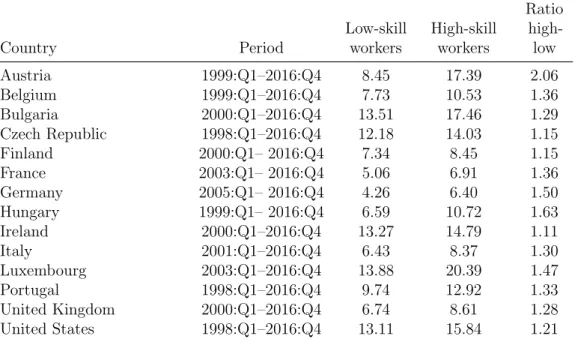
In Table 2.1 we present evidence of a volatility gap in the cyclical component of the unemployment rates of high-skill and low-skill workers in the United States

(18)

Table 2.1: Cyclical volatility of the unemployment rate in the United States and thirteen E.U. countries, by skill group

Country Period Low-skill workers High-skill workers Ratio high-low Austria 1999:Q1–2016:Q4 8.45 17.39 2.06 Belgium 1999:Q1–2016:Q4 7.73 10.53 1.36 Bulgaria 2000:Q1–2016:Q4 13.51 17.46 1.29 Czech Republic 1998:Q1–2016:Q4 12.18 14.03 1.15 Finland 2000:Q1– 2016:Q4 7.34 8.45 1.15 France 2003:Q1– 2016:Q4 5.06 6.91 1.36 Germany 2005:Q1– 2016:Q4 4.26 6.40 1.50 Hungary 1999:Q1– 2016:Q4 6.59 10.72 1.63 Ireland 2000:Q1–2016:Q4 13.27 14.79 1.11 Italy 2001:Q1–2016:Q4 6.43 8.37 1.30 Luxembourg 2003:Q1–2016:Q4 13.88 20.39 1.47 Portugal 1998:Q1–2016:Q4 9.74 12.92 1.33 United Kingdom 2000:Q1–2016:Q4 6.74 8.61 1.28 United States 1998:Q1–2016:Q4 13.11 15.84 1.21

Notes: The statistics reported are standard deviations (in percent). Data are log-transformed quarterly unemployment rates, presented as deviations from a Hodrick-Prescott filtered trend with the smoothing parameter set to 1600. Data for the United States are obtained from monthly series of the Current Population Survey, and data for the E.U. countries are from the European Union Labor Force Survey. See the text for additional details.

and thirteen European Union countries. The data are seasonally adjusted quarterly log unemployment rates, presented as deviations from an Hodrick-Prescott filtered trend with the smoothing parameter set to 1600.1 _{For the United States the data} are computed from monthly series of the Current Population Survey, and for the E.U. countries the data are from the European Union Labor Force Survey. In all countries the data refers to individuals aged between 20 and 64 years old, which we categorize as high-skill workers if the data indicates they have completed at least 4 years of college education (U.S. data) or tertiary education (E.U. data), and as low-skill workers otherwise. The samples for the E.U. countries are dictated by data availability; the sample for the United States begins at the earliest year for which there is data available for the E.U. countries. We can see that in some cases – like in the Czech Republic, Finland, and Ireland – the standard deviation of the detrended log unemployment rate is around 10% to 15% larger for high-skill workers than for low-skill workers. In other cases – like in Austria, Germany or Hungary – the di↵erence is much more substantial, with the standard deviation of the detrended log unemployment rate being at least 50% larger for high-skill workers. Across all

1_{We present results obtained from data on unemployment rates, but there is no meaningful}

di↵erence if we use data on unemployment levels.

(19)

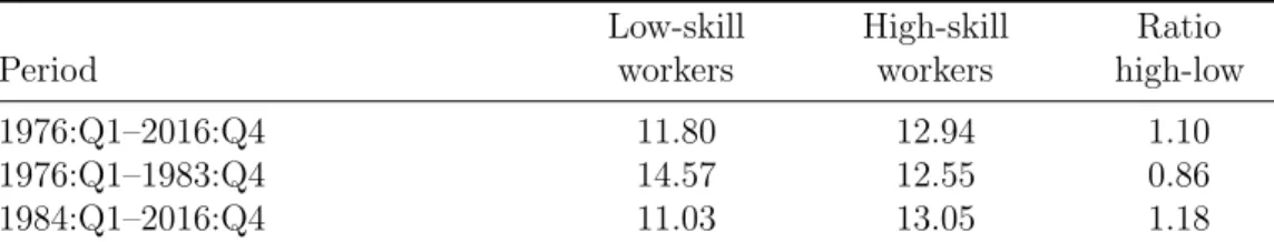
Table 2.2: Cyclical volatility of the unemployment rate in the United States, by skill group

Period Low-skill workers High-skill workers Ratio high-low 1976:Q1–2016:Q4 11.80 12.94 1.10 1976:Q1–1983:Q4 14.57 12.55 0.86 1984:Q1–2016:Q4 11.03 13.05 1.18

Notes: The statistics reported are standard deviations (in percent). Data are log-transformed quarterly unemployment rates, presented as deviations from a Hodrick-Prescott filtered trend with the smoothing parameter set to 1600. Data are obtained from monthly series of the Current Population Survey. See the text for additional details.

countries, the business cycle volatility of the unemployment rate is on average 37% higher for high-skill workers than for low-skill workers, and a Wilcoxon signed-rank test shows that the di↵erence is statistically significant at the 1% level (z = 3.296, p = 0.001).2

For the United States the availability of data allows us to extend our analysis to a longer period of time, and in Table 2.2 we present additional evidence regarding the volatility gap in the detrended log unemployment rates of low-skill and high-skill workers. Over the period 1976:Q1–2016:Q4, the standard deviation of the unemployment rate is 10% larger for high-skill workers than for low-skill workers, a gap which is smaller than the 21% gap observed over the period 1998:Q1–2016:Q4. This suggests that the unemployment volatility gap in the United States experienced a change some time between the first quarter of 1976 and the last quarter of 2016. This is perhaps unsurprising, as the literature documents several instances of volatility shifts in time series of the United States economy during the mid-1980s. For example, Kim and Nelson (1999) and McConnell and Perez-Quiros (2000) provide evidence that points to a decline in the volatility of the growth rate of the U.S. GDP after the first quarter of 1984. Stock and Watson (2002) present evidence of similar declines in several other time series of the United States economy. More recently, Castro and Coen-Pirani (2008) document a threefold increase in the cyclical volatility of skilled hours relative to the cyclical volatility of GDP in the United States since 1984, and Champagne and Kurmann (2013) show that the business cycle volatility of the average real hourly wage increased at least 30% since 1984.

Accordingly, in Table 2.2 we also present results for two sub-periods of the U.S. data

2_{The di↵erence between the standard deviations of the detrended log unemployment rates of}

high-skill and low-skill workers across countries remains statistically significant at the 1% level on a Wilcoxon signed-rank test (z = 2.934, p = 0.0033) even if we exclude the observations relative to France, Germany and Luxembourg – three countries for which the results are obtained from smaller samples and may therefore be less reliable.

(20)

Figure 2.1: Cyclical volatility of the unemployment rate in the United States, 40-quarters-ahead, by skill group

1976 1980 1984 1988 1992 1996 2000 2004 0 5 10 15 20 25 Standard de viation (in p erc en t) High-skill Low-skill

created by splitting the sample in the first quarter of 1984. In the 1976:Q1–1983:Q4 sub-period, the volatility of the detrended log unemployment rate is about 14% lower for high-skill workers than for low-skill workers. In contrast, in the 1984:Q1–2016:Q4 sub-period the detrended log unemployment rate is 18% more volatile for high-skill workers than for low-skill workers. The change is mostly driven by a decrease in the standard deviation for low-skill workers (from 14.57 to 11.03), as there is only a slight increase in the standard deviation for high-skill workers (from 12.55 to 13.05). In Figure 2.1 we o↵er another perspective of the change in the relative size of the cyclical volatilities of the unemployment rates of high-skill and low-skill workers. The lines depict 10-years-ahead rolling-window standard deviations of the detrended log unemployment rate. We can see that the forward volatility is initially lower for high-skill workers, but the gap relative to low-skill workers fades as we enter the 1980s, and by the mid-1980s the 10-years-ahead volatility is slightly higher for high-skill workers. The gap widens in the early and mid-1990s and remains large for the rest of the sample, with the 10-years-ahead volatility being 15% higher for high-skill workers than for low-skill workers at the end of the sample.

In this paper we generalize the framework proposed by C¸ enesiz and Guimar˜aes (2017) to a context of two-skill groups, and we use this setup to address the di↵erences in the cyclical volatility of the unemployment rates of high-skill and low-skill workers. We consider an economy in which households have a variety of high-skill and low-skill workers, each o↵ering a specific low-skill from which monopolistic profits can be derived. Households bear the cost of searching and finding new jobs, and they decide how many new high-skill and low-skill jobs are created each period. While costly, expanding the labor supply on the extensive margin (i.e., employment) benefits the

(21)

household by increasing the number of skill varieties that yield monopolistic profits. On the production side, we assume that firms employ capital and a labor bundle that consists of hours of work from a variety of high-skill and low-skill workers. We assume that firms have a taste for variety with respect to their labor inputs, and this materializes in higher productivity when a wider array of skills is used.

Unemployment dynamics in our model are dictated by two forces. When a positive technology shock hits the economy both productivity and wages increase, raising the value of the marginal new (high-skill or low-kill) job from which the household may extract monopolistic profits. This allows households to o↵set the corresponding search costs for those new jobs, creating an incentive for employment to expand. On the firm side, employment expansion is also attractive because of the increasing returns to employment implied by the firm’s taste for variety. In a calibration of our model to the United States data for the period 1976:Q1–2016:Q4, job search costs are relatively larger for high-skill workers than for low-skill workers. Yet, in the aftermath of a positive technology shock employment expansion relative to the steady state is similar for high-skill and low-skill workers. Higher unemployment rate volatility for high-skill workers then follows from their lower average unemployment rate.

The numerical simulations of the calibrated model generate a volatility of the unemployment rate that is 11.4% higher for high-skill workers than for low-skill workers, a di↵erence that is close to the 9.6% di↵erence observed in the data. Both results are robust to di↵erent calibrations of the Frisch elasticity, as well as to di↵erent calibrations of the parameter that governs the firms’ taste for variety and the size of the monopolistic profits earned by households when exploiting each skill variety. However, our results indicate that the model cannot easily explain the shift in the volatility patterns of the unemployment rates that occurred in the United States during the mid-1980s and early 1990s.

Research that examines di↵erences in the volatility of the unemployment between high-skill and low-skill workers is relatively scarce, but some studies consider the volatility gap in other contexts. Mukoyama and S¸ahin (2006) study di↵erences in the costs of business cycles for high-skill and low-skill workers in a model with incomplete markets and skill heterogeneity, and conclude that the costs of business cycles are between three and ten times larger for unskilled workers. In their model, however, the transitions into and out of unemployment are determined exogenously, and imply higher volatility of the unemployment rate for low-skill workers. In contrast, in our model transitions out of unemployment are determined by the decisions of the

(22)

households with respect to job search, and thus unemployment volatility is determined endogenously. More recently, Hagedorn et al. (2016) introduce skill heterogeneity and capital-skill complementarity (as in Krusell et al., 2000) in a standard search and matching model to examine the e↵ects of taxes on unemployment. They argue that capital-skill complementarity amplifies the volatility of productivity for high-skill workers, driving unemployment volatility upwards, and that higher taxes improve the relative productivity of low-skill, shifting rises in the unemployment to high-skill workers. In our model, unemployment volatility is instead amplified by the presence of economic gains associated with the expansion of employment – both for households, in the form of monopolistic profits over each skill variety, and for firms, in the form of a variety e↵ect that increases productivity.

To some extent, our paper is also related to the literature on the unemployment volatility puzzle. In his influential contribution, Shimer (2005) shows that the business cycle volatility of U.S. unemployment is about 20 times larger than the business volatility of unemployment generated by the Mortensen and Pissarides (1994) search and matching model. This finding has spawned a large literature that aims at improving the amplification mechanism of the search and matching framework. A set of studies argues that some form of wage rigidity is necessary to generate realistic unemployment fluctuations. A few examples of this line of research include the role bargaining delays emphasized by Hall and Milgrom (2008), the staggered wage bargaining proposed by Gertler and Trigari (2009), or the presence of information asymmetries proposed by Kennan (2010). Hagedorn and Manovskii (2008), on the other hand, argue that an alternative calibration for value of non-market activity and the workers’ bargaining weight are sufficient to increase unemployment volatility on the canonical search and matching model. Pissarides (2009) emphasizes instead that fixed matching costs can increase the volatility of unemployment while retaining the wage flexibility for new matches observed in the data. More recently, Petrosky-Nadeau and Wasmer (2013) support Pissarides’ view by arguing that financial frictions generate an entry cost to job creation, and that such cost increases volatility in the labor market.

Our paper makes a contribution to this discussion by introducing an alternative framework to model unemployment in an otherwise standard real business cycle model. Unlike the standard search and matching model, in which wage increases that occur in response to a positive shock discourage firms from creating jobs, the mechanisms in our model combine to favor employment expansion and amplify volatility in the labor market. On the firm side the variety e↵ect raises productivity

(23)

when employment expands, o↵setting the detrimental e↵ects of wage increases on job creation. On the household side the expansion of employment increases the number of skill varieties from which monopolistic profits can be derived, o↵setting the costs of searching for new jobs. The model calibrated for the period 1976:Q1–2016:Q1 generates realistic business cycle volatility for the U.S. unemployment rates. For high-skill workers the unemployment rate is about 9.4 times more volatile than output in the data, and about 8.9 times more volatile than output in the simulations of the model. For low-skill workers the unemployment rate is about 8.6 times more volatile than output in the data, and about 8.1 times more volatile than output in the simulations of the model.

The rest of the paper is organized as follows. In Section 2.2 we present the model and describe its competitive equilibrium. In Section 2.3 we discuss how we calibrate the model to United States data. In Section 2.4 we compare the results of our numerical simulations with the data. In Section 2.5 we perform a sensitivity analysis with respect to a set of key parameters. We close with some concluding remarks in Section 2.6.

2.2 Model

For ease of exposition and notation, in what follows we use the term skilled to refer to high-skill workers. We denote any variable that relates to skilled workers with the subscript s. Similarly, we use the term unskilled to refer to low-skill workers. We denote any variable that relates to unskilled workers with the subscript u. We assume that households live infinitely, and time is discrete and indexed by t 0.

2.2.1 Firms

The technology of a representative firm is described by a Cobb-Douglas function:

yt= atkt↵l1 ↵t , (2.1)

where yt is the output of final goods, ktis the capital input, lt is the labor input, and at is a common productivity factor. The parameter ↵ is the capital share, 0 < ↵ < 1. The law of motion of the common productivity factor is given by:

(24)

where ✏t is an i.i.d. productivity shock, ✏t⇠ N (0, ✏) for all t 0. The labor input lt is a composite of skilled labor, ls,t, and unskilled labor, lu,t:

lt= ls,tlu,t1 , (2.3)

where 0 < < 1.

The input lu,t is a composite of hours of work, and is described by a constant elasticity of substitution function over a continuum of unskilled workers indexed by j:

lu,t = " j2Ju,t hu,t(j)✓dj #1 ✓ , (2.4)

where hu,t(j) are the hours worked by the j-th unskilled worker, Ju,t is the set of unskilled workers employed by the firm at time t, and 1/ (1 ✓) is the elasticity of substitution between any two unskilled workers. Because our model features unemployment, Ju,t is a subset of all existing unskilled workers, Ju,t ⇢ Ju. The input ls,t is defined in a similar way:

ls,t = " j2Js,t (!hs,t(j))✓dj #1 ✓ , (2.5)

where hs,t(j) are the hours worked by the j-th skilled worker, Js,t ⇢ Js is the set of skilled workers employed by the firm at time t, and 1/ (1 ✓) is the elasticity of substitution between any two skilled workers, 0 < ✓ < 1. The parameter ! > 1 captures a productivity advantage of skilled workers relative to unskilled workers. The firm sells its output in a perfectly competitive market, and – given the law of motion of the common productivity factor – it solves:

max yt,kt,lt,lu,t,ls,t,hu,t(j),hs,t(j) yt rtkt j2Ju,t wu,t(j) hu,t(j) dj j2Js,t ws,t(j) hs,t(j) dj, (2.6) subject to (2.1) and (2.3)–(2.5), where rt is the rental rate of capital, wu,t(j) is the hourly wage paid to the j-th unskilled worker, and ws,t(j) is the hourly wage paid to the j-th skilled worker. The first order conditions of the firm’s maximization problem imply: rt= ↵ yt kt (2.7) 12

(25)

Wu,t = " j2Ju,t wu,t(j) ✓ ✓ 1dj #✓ 1 ✓ (2.8) Ws,t= ! 1 " j2Js,t ws,t(j) ✓ ✓ 1dj #✓ 1 ✓ (2.9) Wu,t = (1 ↵) (1 ) yt lu,t (2.10) Ws,t= (1 ↵) yt ls,t (2.11) hu,t(j) =  wu,t(j) Wu,t 1 ✓ 1 lu,t (2.12) hs,t(j) =  ws,t(j) Ws,t ! ✓ 1 ✓ 1 ls,t (2.13)

where Wu,t is the unskilled wage index, as defined in (2.8), and Ws,t is the skilled wage index, as defined in (2.9).

2.2.2

Households

The representative household is composed of a continuum of unskilled members of mass Nu_{, and a continuum of skilled members of mass N}s_{, with N}u_{+ N}s _{= 1; both} types of household members are indexed by a variety index j. At any given time t a fraction nu,t 2 [0, Nu] of unskilled members and a fraction ns,t2 [0, Ns] of skilled members are employed. As in Merz (1995), household members pool their income as a mechanism to completely insure each other against unemployment. The period utility of the household is given by:

Ut= log ct nu,t 0 u (hu,t)1+ u 1 + u dj ns,t 0 s hs,t(j)1+ s 1 + s dj, (2.14)

where ctis the consumption of the household, 1/ sand 1/ u are the Frisch elasticities of labor supply for skilled and unskilled household members, and s and u are measures of the disutility of work for skilled and unskilled household members. At the end of any given period t a fraction of the household members who are employed lose their jobs. The household members who are unemployed engage in a costly search for new jobs, and thus nu,t and ns,t change over time in response to the interplay between job destruction and job creation. The law of motion of nu,t is

(26)

given by:

nu,t = (1 u) nu,t 1+ xu,t, (2.15)

where u is the fraction of unskilled workers who lose their jobs, and xu,t are the new jobs for unskilled members at time t. Likewise, the law of motion of ns,t is given by:

ns,t = (1 s) ns,t 1+ xs,t, (2.16)

where s is the fraction of unskilled workers who lose their jobs, and xs,t are the new jobs for unskilled members at time t. The laws of motion (2.15) and (2.16) imply that new jobs created at time t become immediately productive. In this economy, unskilled unemployment is given by qu,t = (Nu nu,t), the skilled unemployment is given by qs,t = (Ns ns,t), and aggregate unemployment is given by qt⌘ qs,t+ qu,t = 1 ns,t nu,t. The unemployment rates of skilled and unskilled workers are given by us,t = q_Ns,tS and uu,t = q_Nu,tU, respectively.

The household holds a stock of capital for which the law of motion is:

kt+1= (1 k) kt+ it, (2.17)

where k is the constant depreciation rate, and it is the household’s investment. The household spends its income on consumption, investment, and costly job searching activities for unskilled and skilled workers who are unemployed. The budget constrain of the household is given by:

ct+it+gu,t(xu,t)+gs,t(xs,t) nu,t 0 wu,t(j) hu,t(j) dj+ ns,t 0 ws,t(j) hs,t(j) dj+rk,tkt, (2.18) where gu,t(xu,t) and gs,t(xs,t) are strictly increasing functions that measure the costs of finding unskilled and skilled jobs, respectively. We assume that these costs are quadratic in the number of new jobs created at time t:

gu,t(xu,t) = u ✓ xu,t+ 1 2x 2 u,t ◆ (2.19) gs,t(xs,t) = s ✓ xs,t+ 1 2x 2 s,t ◆ (2.20) with u, s > 0. 14

(27)

The household solves:

max

ct,kt+1,nu,t,ns,t,hu,t(j),hs,t(j),wu,t(j),ws,t(j)

E0 1 X t=0 t_U t (2.21)

subject to (2.12)–(2.13) and (2.15)–(2.20), where is the common discount factor in the economy. We anticipate an equilibrium in which there is symmetry across unskilled workers, and symmetry across skilled workers. For unskilled workers we have wu,t(j) = wu,t and hu,t(j) = hu,t, 8j 2 [0, nu,t]; for skilled workers we have ws,t(j) = ws,t and hs,t(j) = hs,t, 8j 2 [0, ns,t]. The first order conditions of the household’s maximization problem imply:

1 = Et  ct ct+1 (1 k+ rk,t+1) (2.22) wu,t = cthu,tu u ✓ (2.23) ws,t = cths,ts s ✓ (2.24)

g0_u,t(xu,t) = wu,thu,t

1 + u ✓ 1 + u + Et  (1 u) ct ct+1 g_u,t0 (xu,t+1) (2.25) g0_s,t(xs,t) = ws,ths,t 1 + s ✓ 1 + s + Et  (1 s) ct ct+1 g_s,t0 (xs,t+1) (2.26)

where g_u,t0 = @gu,t/@xu,t and g

0

s,t= @gs,t/@xs,t, 8t 0.

An aggregate resource constraint closes the model of the economy:

ct+ it+ gu,t(xu,t) + gs,t(xs,t) yt. (2.27)

2.2.3

Competitive equilibrium

A competitive equilibrium for this economy is a sequence of prices _{rt, wst, wtu}1t=0 and allocations_{yt, ct, kt+1, lt, ls,t, lu,t, nu,t, ns,t, xu,t, xs,t}1_t=0such that firms solve (2.6) subject to 2.1 and 2.3–2.5, households solve (2.21) subject to (2.12)–(2.13) and (2.15)–(2.20), the aggregate resource constraint binds, and:

lu,t =  nu,t 0 hu,t(j)✓dj 1 ✓

(28)

ls,t=  ns,t 0 (!hs,t(j))✓dj 1 ✓

given the exogenous process for the common productivity factor described in (2.2). In the symmetric competitive equilibrium the unskilled and skilled labor inputs used by the firm and the

lu,t = hu,t(nu,t)

1

✓ (2.28)

ls,t = !hs,t(ns,t)

1

✓ _(2.29)

Wu,t = wu,t(nu,t)

✓ 1

✓ (2.30)

Ws,t = ! 1ws,t(ns,t)

✓ 1

✓ . (2.31)

The results (2.28) and (2.29) highlight how the assumption that firms have a taste for skill variety within each skill group leads to increasing returns to scale in the unskilled and skilled labor inputs.

2.3 Calibration

In this section we describe the baseline calibration used in our numerical simulations. We calibrate the model to United States data and define the quarter as the unit of time. Table 2.3 summarizes the baseline parameter values. For some of the parameters we use values that are standard in the business cycle literature. We set the capital share ↵ to 0.36. We set the discount factor to 0.99 so that annual interest rate is 4% in the steady state. We set the depreciation rate k to 0.025 so that capital depreciation approximates 10% annually. Finally, for the law of motion of technology we use ✏ = 0.007 and ⇢ = 0.95.

For the inverse of the Frisch elasticities our baseline calibration considers s= u = 1.5, which implies Frisch elasticities of 0.67 for both skilled and unskilled workers. There is considerable debate about the value of the Frisch elasticity: studies based on microeconomic data typically yield estimates well bellow 1, while macroeconomic models often require values in excess of 2 to match the business cycle volatility observed in the data (see, e.g., Chetty et al. (2011) for a discussion of the mismatch between micro and macro estimates). Given this lack of consensus and considering that the behavior of the labor market variables is likely to be a↵ected by the Frisch elasticities, in Section 2.5 we include s and u in our sensitivity analysis.

To calibrate the separation rates u and s we turn to empirical estimates available 16

(29)

in the literature. Chassamboulli (2011) estimates monthly separation rates using data from the Job Openings and Labor Turnover Survey covering the period between December 2000 and October 2010, finding a separation rate of 0.016 for high-skill workers and a separation rate of 0.035 for low-skill workers. At quarterly frequency these estimates imply a separation rate of 0.047 for high-skill workers and a separation rate of 0.101 for low-skill workers. More recently, Hagedorn et al. (2016) estimate monthly separation rates using data from the Current Population Survey covering the period between January 1976 and December 2006 and obtain similar results. Their estimates indicate a separation rate of 0.0097 for high-skill workers and a separation rate of 0.0378 for low-skill workers. At quarterly frequency these estimates imply a separation rate of 0.029 for high-skill workers and a separation rate of 0.109 for low-skill workers. We consider an average of these two estimates and set s = 0.038 and u = 0.105. In our model these values imply that in any given quarter 3.8% of the skilled workers and 10.5% of the unskilled workers lose their jobs.

We set = 0.4 so that skilled workers receive 40% of the total wage bill. This number is consistent with estimates available in the literature for the share of the wage bill earned by high-skill workers. For example, Machin and Van Reenen (1998) show that in the United States the share of the wage bill paid to non-production workers (a proxy for high-skill workers) was 41.4% in 1989. More recently Chongvilaivan et al. (2009) show that, according to data from the 2002 Annual Survey of Manufactures

published by the U.S. Census Bureau, high-skill workers receive 39.9% of the wage bill.

For the productivity advantage of skilled workers relative to unskilled workers, !, we turn to estimates from the literature on skill-related wage di↵erences. For example, Katz and Murphy (1992) show that the wage premium of college educated workers (a proxy for high-skill workers) in the U.S. was between 50% and 70% relative to non-college educated workers during the period between the early 1960s to the late 1980s. In another study, Berman et al. (1998) find that the wages of non-production workers (a proxy for high-skill workers) are about 50% higher than the wages of production workers (a proxy for low-skill workers) in OECD countries. More recently, van der Velden and Bijlsma (2016) estimate that in a sample of 22 OECD countries workers with a college degree earn, on average, almost 30% more than workers without a college degree. To the extent that di↵erences in wages reflect di↵erences in worker productivity, these estimates would suggest that the productivity advantage of skilled workers relative to unskilled workers is between 30% and 70%. Accordingly, in our baseline calibration we set ! = 1.5.

(30)

Table 2.3: Baseline calibration

Description Parameter Value

Firms:

Capital’s income share ↵ 0.36

Capital depreciation rate k 0.025

Productivity advantage of skilled workers ! 1.5

Skilled workers’ wage bill share 0.40

Elasticity of substitution between workers of same type

1/ (1 ✓) 6.67

Households:

Discount factor 0.99

Inverse of the Frisch elasticity s, u 1.5

Separation rate for skilled workers s 0.038

Separation rate for unskilled workers u 0.105

Search cost parameter for skilled jobs s 25.7

Search cost parameter for unskilled jobs u 5.1

Scaling of disutility from skilled work s 2.4

Scaling of disutility from unskilled work u 1.2

Technology:

Standard deviation of technology shock ✏ 0.007

Persistence of the technology process ⇢ 0.95

For the parameter ✓ there are no obvious empirical estimates available in the literature. In our baseline calibration we set ✓ = 0.85, which implies an elasticity of substitution of 6.7 between any two workers in the same skill group, and in Section 2.5 we include this parameter in our sensitivity analysis. We use the remaining four parameters ( s, u, s, and u) to normalize hours worked to one for both skilled and unskilled workers, and to target the average unemployment rates of skilled and unskilled workers in the United States in the period 1976:Q1–2016:Q4, which are 2.9% and 6.8%, respectively.3 _{This yields the calibration}

s = 2.4, u = 1.2, s = 25.7, and u = 5.1. This calibration implies that households face job search costs that are higher for skilled workers than for unskilled workers. Intuitively, this is a reasonable assumption: skilled jobs are likely to be more complex than unskilled jobs, and skilled workers are likely be required to go through more rounds of screening than unskilled workers to ensure a correct match to a new job, resulting in higher search costs for skilled workers.

3_{The Appendix illustrates how we use the hours normalization and our target unemployment}

rates to pin down s, u, s, and u.

(31)

2.4 Results

2.4.1 Business cycle properties

In this section we compare the business cycle properties of the calibrated model with the business cycle properties of U.S. data covering the period 1976:Q1–2016:Q4. While our focus is on the volatility of the unemployment rates of skilled and unskilled workers, we also examine the behavior of other macroeconomic aggregates. We run 1000 model simulations of as many quarters as in the U.S. sample (164 quarters), and for each simulation we compute standard deviations, autocorrelations, and cross-correlations (with output) for the unemployment rates, output, consumption and investment. The results we report for the model are the means of the simulated statistics. To compute the equivalent statistics for the U.S. economy we use data on output, consumption and investment published by the Bureau of Economic Analysis, and data on the unemployment rates computed from monthly series of the Current Population Survey. All variables are log-transformed and presented as deviations from a Hodrick-Prescott filtered trend with the smoothing parameter set to 1600. We present the results in Table 2.4.

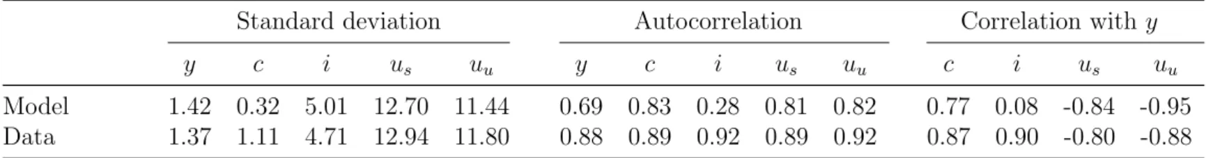
The calibrated model replicates the business cycle volatility of the unemployment rates quite well. The simulated standard deviation of the unemployment rate is 12.70 for skilled workers and 11.44 for unskilled workers, a di↵erence that makes the business cycle volatility 11% larger for skilled workers. In the data, the standard deviation of the unemployment rate is 12.94 for skilled workers and 11.80 for unskilled workers, a di↵erence that makes the business cycle volatility around 10% larger for skilled workers. Moreover, in the model the unemployment rates are substantially more volatile than output, and the volatility ratios are close to those we observe in the data. For skilled workers, the unemployment rate is 8.9 times more volatile than output in our simulations, and 9.4 times more volatile than output in the data. For unskilled workers, the unemployment rate is 8.1 times more volatile than output in our simulations, and 8.6 times more volatile than output in the data. Thus, in terms of the business cycle volatility of unemployment our model outperforms the canonical search and matching model of Mortensen and Pissarides (1994).

The model also generates realistic business cycle volatility for the time series of output and investment. The simulated standard deviations of output and investment are 1.42 and 5.01, respectively, whereas the corresponding standard deviations in the data are 1.37 and 4.71. Even though the model slightly overestimates the volatility of

(32)

Table 2.4: Standard deviations, autocorrelations and cross correlations with output, from model simulations and U.S. data, 1976:Q1–2016:Q4

Standard deviation Autocorrelation Correlation with y

y c i us uu y c i us uu c i us uu

Model 1.42 0.32 5.01 12.70 11.44 0.69 0.83 0.28 0.81 0.82 0.77 0.08 -0.84 -0.95

Data 1.37 1.11 4.71 12.94 11.80 0.88 0.89 0.92 0.89 0.92 0.87 0.90 -0.80 -0.88

Notes: Standard deviations are in percent. The row labelled “Data” refers to United States quarterly data for the period 1976:Q1– 2016:Q4. The series for output (y), consumption (c) and investment (i) are from the Bureau of Economic Analysis. The series for the quarterly unemployment rates (us, uu) are computed from monthly series of the Current Population Survey. The row labelled “Model”

refers to results from 1000 model simulations of 164 quarters each, which is the same number of quarters as in the U.S. sample. The results are sample means of the statistics computed for each of the 1000 simulations. All variables are log-transformed and presented as deviations from a Hodrick-Prescott filtered trend with the smoothing parameter set to 1600.

(33)

both variables, it approximates the relative volatility of investment remarkably well: the time series for investment is 3.5 more volatile than output in the model, and 3.4 times more volatile than output in the data. One shortcoming of our model is that it generates time series for consumption that are too smooth. The simulated standard deviation of consumption is 0.32, whereas in the data the standard deviation is 1.11, about 3.5 times larger.

Turning to the simulated first-order autocorrelation coefficients, we see that for all variables presented in Table 2.4 the model generates coefficients that are smaller than those we estimate from the data. The model performs best when replicating the autocorrelation of the unemployment rates and consumption. For the unemployment rates of skilled and unskilled workers the simulated autocorrelation coefficients are 0.81 and 0.82, respectively, and for consumption the coefficient is 0.83. In all three cases the simulated coefficients are about 10% smaller than the corresponding coefficients estimated from the data. The model performs worse when replicating the autocorrelation of output and investment. The simulated autocorrelation coefficients are 0.69 for output and 0.28 for investment, whereas in the data the coefficients are 0.88 and 0.92. The di↵erence is particularly striking for investment, with the coefficient estimated from the data being 3.3 times larger than the simulated coefficient. Furthermore, the autocorrelation of the simulated time series is much smaller for investment than for output, whereas in the data the autocorrelation coefficient is slightly larger for investment than for output.

The model generates reasonable cross correlations between output and the unem-ployment rates. For skilled workers the cross correlation is -0.84 in the model and -0.80 in the data. For unskilled workers the cross correlation is -0.95 in the model and -0.88 in the data. Although the simulated cross correlations are between 5% and 8% larger than what we observe in the data, the model correctly generates a cross correlation between output and the unemployment rate that is larger for unskilled workers. The simulated co-movement of output and consumption is also plausible, with the model generating a cross correlation of 0.77 between the two variables, a figure that is about 12% smaller than its equivalent in the data. However, the model performs poorly in terms of the cross correlation between output and investment. In the data the two variables exhibit very tight co-movement, but in the calibrated model we obtain a very small positive cross correlation.

(34)

Figure 2.2: Response of selected model variables to an exogenous technology shock 20 40 60 80 30 20 10 0 us 20 40 60 80 0 0.5 1 1.5 2 c 20 40 60 80 0 0.5 1 1.5 2 y 20 40 60 80 1 0.5 0 0.5 1 ns 20 40 60 80 1 0.5 0 0.5 1 nu 20 40 60 80 30 20 10 0 uu 20 40 60 80 1 0.5 0 0.5 1 hu 20 40 60 80 1 0.5 0 0.5 1 hs 20 40 60 80 0 1 2 3 4 i 20 40 60 80 0 0.5 1 1.5 2 l 20 40 60 80 0 0.2 0.4 0.6 0.8 1 ws 20 40 60 80 0 0.2 0.4 0.6 0.8 1 wu

Notes: The dashed lines represent the response of selected model variables to a one standard deviation ( ✏= 0.007) exogenous technology shock. The horizontal axis measures the number of

periods after the shock. All variables are presented as percent deviations from their respective steady state values.

2.4.2 Impulse response functions

We now analyze how a set of model variables behave in response to an exogenous technology shock. In Figure 2.2 we depict the response of output, consumption, investment, employment, unemployment, hours worked, and wages to a one standard deviation positive technology shock in our calibrated model. All variables as presented as percent deviations from their steady state values. In the top three panels, we see that the shock produces the usual e↵ects on output, consumption and investment: all three variables increase after the shock hits the economy, and then gradually return to their steady state values. Thus, with respect to these variables our model essentially retains the responses typically observed in a standard business cycle model.

When the shock hits the economy, skilled employment initially increases less than

(35)

unskilled employment because the cost of searching for new jobs is relatively higher for skilled workers than for unskilled workers. This initial expansion in employment gives rise to the variety e↵ect on the firms’ side and contributes to increase productivity. This, in turn, drives further employment expansions by making the marginal new job (skilled or unskilled) valuable enough to o↵set the respective search cost. Because of the complementarity between skilled and unskilled labor in the firms’ labor bundle, the expansion of unskilled employment increases the productivity of skilled workers. As a result, more new skilled jobs are now valuable enough to o↵set their corresponding search costs, and additional expansions of skilled employment become economically attractive for the households. While the same e↵ect exists for unskilled workers, the strong initial expansion driven by the lower search costs reduces the scope for additional employment growth. These dynamics cause skilled employment to peak later than unskilled employment, although they both expand by around 0.8% relative to their steady state values.

Because the unemployment rate of skilled workers is lower than the employment rate of unskilled workers, the employment growth results in a stronger compression of the unemployment rate for skilled workers than for unskilled workers. At the peak of skilled employment expansion, the unemployment rate for skilled workers is compressed by around 26% relative to its steady state value. In contrast, at the peak of unskilled employment expansion, the unemployment rate for unskilled workers is compressed by only 11% relative to its steady state value.

When the exogenous shock hits the economy, hours worked increase for skilled and unskilled workers. The productivity shock increases the value of market work and creates an incentive to substitute leisure for labor. As employment expands, the number of skill varieties from which households derive monopolistic profits increases, and the resulting gains allow households to shift part of the labor supply from the intensive margin (hours) to the extensive margin (employment). The initial increase in hours is slightly larger for skilled workers: relative to the steady state, skilled hours expand by as much as 0.28%, whereas unskilled hours expand by as much as 0.18%. Wages respond to the exogenous shock with a profile similar to that of output, increasing when the shock hits the economy and then gradually converging back to their steady state value. For unskilled workers, the stronger employment expansion immediately after the shock is associated with a steeper compression of the wages early on, but smoother declines in subsequent periods.

(36)

2.4.3 Unemployment rate volatility: pre-1984 and post-1984

2.4.3.1 Baseline simulations

In Section 2.1 we have seen that, starting in the mid-1980s, the business cycle volatility of the U.S unemployment rates experienced some changes. The unemployment rate was slightly more volatile for low-skill workers than for high-skill workers in the 1976:Q1–1983:Q4 sub-period, but more volatile for high-skill workers in the 1984:Q1–2016:Q4 sub-period. These patterns of volatility take place against di↵erent labor market conditions. The first di↵erence, although small, pertains to the unemployment rates themselves. In the pre-1984 sub-period the unemployment rates averaged 2.9% for high-skill workers and 6.7% for low-skill workers; in the post-1984 sub-period they averaged 3.1% for high-skill workers and 7.5% for low-skill workers. The second di↵erence, much more substantial, pertains to the share of high-skill workers in the labor force. In the pre-1984 sub-period the share of high-skill workers in the labor force averaged 17.2%, whereas in the post-1984 sub-period that share averaged 26%.

In this section we investigate whether our calibrated model can replicate the di↵erent patterns of volatility of the unemployment rates in the pre-1984 and post-1984 sub-periods. We proceed as before: we run 1000 simulations of as many quarters as in the relevant sub-period (32 quarters in 1976:Q1–1983:Q4, 132 quarters in 1984:Q1–2013:Q4), and for each of the simulations we compute standard deviations, autocorrelations, and cross correlations (with output) for the unemployment rates, output, consumption and investment. We then compute the sample means of the statistics obtained in each of the 1000 simulations, and we compare them to the corresponding statistics computed from the U.S. data. In all simulations we retain the baseline calibration summarized in Table 2.3, except for s, u, s, and u, which we use to normalize hours worked to one and to target the unemployment rates observed in each of the simulated sub-periods.

We present the results of our analysis in Table 2.5. On the simulations for the sub-period 1976:Q1–1983:Q4, the model generates unemployment rates that are more volatile for skilled workers than for unskilled workers, with the standard deviation being about 20% larger for skilled workers. This is in clear contradiction with the U.S. data, which show the business cycle volatility of the unemployment rate to be about 14% lower for skilled workers during that period. On the simulations for the sub-period 1984:Q1–2016:Q4, the model correctly generates a volatility for the

(37)

unemployment rates that is higher for skilled workers than for unskilled workers. However, the simulated volatility gap is about 8%, whereas in the data the volatility gap is about 18%. Moving between sub-periods, the model correctly replicates the increase in the volatility of the unemployment rate of skilled workers, but fails to account for the decrease in the volatility of the unemployment rate of unskilled workers.

For both periods our simulations generate time series that are more volatile for investment than for output. For the sub-period 1976:Q1–1983:Q4 the model yields a volatility ratio of 3.8, exceeding the ratio observed in the data by about 36%. For the period 1984:Q1–2016:Q4 the model performs slightly better, yielding a volatility ratio that is about 13% smaller than the ratio observed in the data. As before, consumption is much smoother in the model than in the U.S. data. For both periods the model simulations yield a volatility for consumption that is about 22% of the volatility of output, whereas in the data the volatility of consumption is between 76% and 85% of the volatility of output. One important mismatch is that, in general, the calibrated model yields lower levels of volatility for output, consumption and investment on the simulations for the 1976:Q1-1983:Q4 sub-period. In contrast, the data show that, in general, the volatility in 1976:Q1-1983:Q4 sub-period is actually higher than in the 1984:Q1–2016:Q4 sub-period. The results, however, are from simulations where the standard deviation of the exogenous technology shock is assumed to remain constant across the two sub-periods, and in light of the evidence presented in the literature (see, e.g., Kim and Nelson, 1999) this assumption might be somewhat problematic. All variables exhibit a lower first-order autocorrelation on the simulations that correspond to the 1976:Q1–1983:Q4 sub-period. For output, consumption, and the unemployment rates, however, the data show that autocorrelations coefficients are only marginally smaller during this period when compared to the post-1984 sub-period. For investment, the results from the model are a qualitative approximation to the data, although the simulated autocorrelation coefficients are substantially smaller than the equivalent coefficients in the data.

Except for investment, the cross correlations with output are not substantially di↵erent across the two sub-periods, both in the calibrated model and in the data. The model generates negative correlations between the unemployment rates and output that approximate the data quite well, and it yields a positive correlation between consumption and output that is only slightly smaller than in the data. As before, the model performs poorly in terms of replicating the correlation between investment and output. For the 1984:Q1–2016:Q4 sub-period the model predicts a

(38)

T a bl e 2 .5 : S t a n d a r d d e v ia t io n s, a u t o c o r r e l a t io n s a n d c r o ss c o r r e l a t io n s w it h o u t p u t , f r o m m o d e l si m u l a t io n s a n d U .S . d a t a , su b-p e r io d a n a ly si s S ta n d ar d d ev ia ti on Au to co rr el at io n C or re la ti on w it h y yc i us uu yc i us uu ci us uu 1976:Q1–1983:Q4 Mo d el 1. 28 0. 28 4. 84 10. 69 8. 90 0. 59 0. 75 0. 18 0. 69 0. 75 0. 79 -0. 03 -0. 86 -0. 94 Data 2.21 1.68 6.12 12.5 5 14.57 0.87 0.88 0.89 0.85 0.91 0.86 0.95 -0.84 -0.95 1984:Q1–2016:Q4 Mo d el 1. 43 0. 32 5. 01 12. 67 11. 68 0. 69 0. 83 0. 29 0. 81 0. 82 0. 77 0. 08 -0. 84 -0. 95 Data 1.07 0.91 4.29 13.0 5 11.03 0.89 0.89 0.94 0.89 0.93 0.88 0.89 -0.85 -0.87 Not es : S tan d ar d d ev iat ion s ar e in p er ce n t. T h e ro w lab el le d “D at a” re fe rs to Un it ed S tat es q u ar te rl y d at a. T h e se ri es for ou tp u t (y ), con su m p -ti on (c ) an d in v es tm en t (i ) ar e fr om th e B u re au of E con om ic An al y si s. T h e se ri es for th e u n em p lo y m en t rat es (u s , uu ) ar e com p u te d fr om m on th ly se ri es of th e C u rr en t P o p u la ti o n S u rvey . T h e ro w lab el le d “M o d el ” re fe rs to re su lt s fr om 1000 m o d el si m u lat ion s of as m an y q u ar te rs as in th e U. S . sam p le s (32 q u ar te rs in 1976: Q 1–1983: Q 4; 132 q u ar te rs in 1984: Q 1–2016: Q 4) . T h e re su lt s ar e sam p le m ean s of th e st at is ti cs com p u te d for eac h of th e 1000 si m u lat ion s. Al l var iab le s ar e log-tr an sf or m ed an d p re se n te d as d ev iat ion s fr om a Ho d ri ck -P re sc ot t fi lt er ed tr en d w it h th e sm o ot h in g p ar am et er se t to 1600. 26

(39)

positive cross-correlation that is much smaller than the correlation observed in the data. For the 1976:Q1–1983:Q4 sub-period the mismatch is more severe, with the model yielding a small negative correlation, whereas in the data the correlation is strongly positive.

With some exceptions, the results presented in this section show that adjusting our baseline calibration to account for di↵erences in the relative supply of skilled workers and in the average unemployment rates across the pre-1984 and post-1984 sub-periods is insufficient to replicate certain features of the U.S. data. Some of the shortcomings of our simulations – such as the failure to replicate the lower volatility of output, consumption and investment in the 1984:Q1–2016:Q4 sub-period – are likely to be unrelated to the key feature of our model (i.e., the framework proposed to model unemployment). Other shortcomings – such as the failure to account for the change in the volatility gap of the unemployment rates of skilled and unskilled workers – speak to the core of our model and therefore warrant further examination.

2.4.3.2 Changing parameter calibration

For the purposes of our study, the key shortcoming of the sub-period simulations lies in the failure to fully account for the changes in the volatility of the unemployment rates. In this section we investigate whether the issue is amenable to di↵erent calibrations of ✓, the parameter which is at the core of our framework to model unemployment. This parameter influences how strong the “taste for variety” is on the firm side, and how large are the monopoly gains that households can extract from each specific skill variety. We examine to what extent a di↵erent calibration for ✓ in each of the sub-periods contributes to improve the fit between the simulations and the U.S. data. As before, we retain the baseline calibration summarized in Table 2.3 for all other parameters except for s, u, s, and u, which we once again use to normalize hours worked to one, and to target the unemployment rates observed in each of the simulated sub-periods.

In Table 2.6 we report results from simulations in which we set ✓ = 0.75 for the sub-period 1976:Q1–1983:Q4, and ✓ = 0.95 for the sub-period 1984:Q1–2016:Q4. For the sub-period 1976:Q1–1983:Q4 the model continues to generate unemployment rates that are more volatile for skilled workers than for unskilled workers, in contrast with the data, although the simulated volatility gap (16%) is somewhat smaller than in our baseline results. For the sub-period 1984:Q1–2016:Q4 the model continues