Road Motion Control Electric Vehicle with Speed
and Torque Observer
Daniel Foito
ESTSetúbal Instituto Politécnico Setúbal Campus do IPS - Estefanilha2910 Setúbal, Portugal daniel.foito@estsetubal.ips.pt
Manuel Gaspar
ESTSetúbal Instituto Politécnico Setúbal Campus do IPS - Estefanilha2910 Setúbal, Portugal manuel.gaspar@estsetubal.ips.pt
V. Fernão Pires
ESTSetúbal Instituto Politécnico SetúbalINESC-ID
Campus do IPS - Estefanilha 2910 Setúbal, Portugal vitor.pires@estsetubal.ips.pt
Abstract -- This paper presents an electric vehicle (EV) with two
independent rear wheel drives and with an electric differential system. A model of the vehicle dynamic model is presented. The electric differential was implemented assuring that, in straight right trajectory, the two wheels drives roll exactly at same velocity and, in curve, the difference between the two velocities assure a vehicle trajectory. A speed and torque observer for DC motor was also proposed and simulated. Analysis and simulation results of the proposed system are presented.
Index Terms –Sensorless, Electric Vehicle, Electronic differential, Observer.
I. INTRODUCTION
In order to meet the targets imposed by the EU, vehicle manufacturers have been developing more efficient Internal Combustion Vehicles (ICV) with better performances, less fuel consumption and reduced CO2 emissions. This measure is part of
the EU strategy to reduce CO2 emissions and ensure greenhouse
gas emission targets under the Kyoto Protocol, as well as solving environmental problems such as global warming. Unfortunately there are no simple or short-term solutions to solve the problems created by oil dependence in the area of road transport, among others. To address these problems it will be necessary a far-reaching transformation in both mentalities and technologies so that drivers can choose electricity or biofuels instead of fuel oil to move their vehicles [1].
In recent years, three different technologies of Electric Vehicles have benefited from great developments in motors, batteries and control strategies, namely: Pure Electric Vehicles (common called only as EVs), Hybrid Electric Vehicles (HEVs) and Fuel cell vehicles (FCVs) [1-3]. Such developments represent strong incentives for better energy efficiency and global environmental protection.
The electric vehicles advantages cannot be summarily limited to environmental issues since the control potentialities and the performance of the electrical machines make possible create EVs not only with better energy efficiency but also with new active safety drive conditions. A general limitation is related to the
battery storage capability. Efficient traction control systems have been studied and implemented in electric vehicles [4-6]. In the field of security systems, various stability controls have been proposed [7-8].
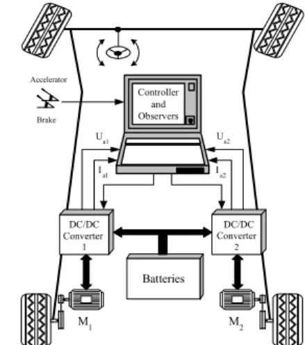
The discussion in this paper is focused on the electric differential controller of an EV with two independent rear drive wheels where the speed applied at each wheel are controlled and based on speed and external torque observers of DC motors. The electric differential control assures the adequate speed rear wheels for vehicle trajectory. In fig. 1 is showed the global strategy proposed for electric differential control of an electric vehicle with two independent rear wheel drives.
This paper is organized as follows. Section 2 presents the vehicle dynamic model and tire model. Section 3 the speed and external torque observers and general controller are described in Section 4. In Section 5 the simulation results are presented. Finally, Section 6 presents the conclusions of the developed work. Accelerator Brake DC/DC Converter 1 DC/DC Converter 2 Batteries M2 M1 I a1 U a1 Ua2 I a2 Controller and Observers
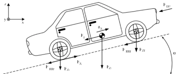
Fig. 1. Propulsion wheel drive control strategy proposed for an EV. II. VEHICLE DYNAMIC MODEL AND TIRE MODEL In order to analysis the dynamic electrical vehicle, it was considered that the traction forces is only associated with rear wheels (fig. 2) [9-10].
Fig. 2. Forces acting on the vehicle moving on slope road. A. Vehicle Dynamic
Equation (1) presents the road load FRT (Driving resistance)
including all the resistant forces opposing to the vehicle motion [2],[3]: I DA RR RT F F F F = + + (1)
where FRR is the rolling resistance force, FDA is the aerodynamic
drag force and FI is the slope resistance (more details in fig. 2).
The equation of longitudinal motion vehicle is defined by equation (2): α ρC A V mgsin F F F V m F F F a m V f D RR X X X RT X X X − − − + = − + = 2 2 1 2 1 2 1 & (2)
B. Wheel and Motor Dynamic
The mechanical equation (in the motor referential) used to describe each wheel drive is expressed by (3) [4].
ext m m m T T dt d J ω = − (3)
In equation (3), ωm is the angular motor speed and Tm the
electromagnetic motor torque. The load torque at the motor referential is defined by (4), where rω is the tire radius, FX is the
traction force and rt is the transmission ratio.
) F F ( r r T RT X t ext= ω + (4)
The moment of inertia of the vehicle from the motor referential Jm, can be defined as a sum of shaft inertia moment
including the motor and wheel inertia Jwheel and the factor
corresponding to the vehicle mass JV:
V wheel
m J J
J = + (5)
The shaft inertia moment JV is defined by equation (6), where
λ is the wheel slip.
) 1 ( i R m 2 1 J 2 2 V = −λ (6)
C. Adhesion Characteristics of Tire and Road The wheel slip λ, is defined by equation (7).
⇒ − = ⇒ − = Braking V V V Driving V V V V V V ω ω ω λ λ (7)
where Vω is the linear velocity of the wheel drive and VV is the
real velocity of the vehicle.
The longitudinal force FX, that each wheel drive tire can
transmit to the road surface is defined by equation (8).
z
X ( )mg ( )F
F =µ λ =µ λ (8)
Fig. 3 shows a simple model of the wheel drive.
Fig. 3. Schematic motion image of wheel drive.
The longitudinal adhesion coefficient between tire and road,
µ, is a function of the slip, λ, approximated by equation (9) [11]. λ λ µ = ⋅ − − ⋅λ − ⋅ 3 1 (1 e 2 ) C C ) ( C (9)
The longitudinal adhesion coefficient, µ, in the tire as function of slip for some road surfaces is showed in Fig. 4.
The slip value, λmáx, corresponds to the maximum adhesion
coefficient between tire and road. Beyond that value, an unstable adhesion coefficient between tire and road is obtained.
TABLE I. TIRE COEFFICIENTS
Asfalt Wet Ice
C1 1,099 0,5495 0,2747
C2 24,98 24,98 24,98
C3 0,299 0,1993 0,1495
D. Electric Differential System
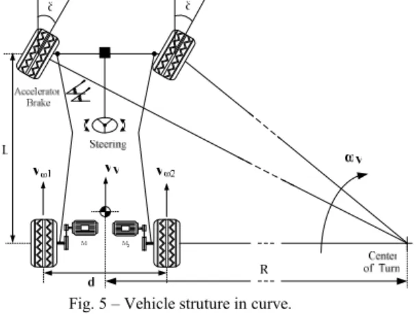
Fig. 5 presents the vehicle structure describing a curve, where L represents the wheelbase, δ the steering angle, d the distance between the wheels of the same axle and ω1 and ω2 the angular speeds of the wheel drives, respectively [12-13].
Fig. 5 – Vehicle struture in curve.
In accordance with fig. 5, the linear speed of each wheel drive is express as a function of the vehicle speed and the radius of turn, by equation (10).
(
)
(
)
− = + = 2 2 2 1 d R V d R V V V ω ω ω ω (10)and the radius of curve depends on the wheelbase and steering angle, by equation (11).
δ
tan L
R = (11)
In accordance with fig. 3 and considering that the slip for each wheel drive is very low, the correspondent wheel speed is imposed by the respective motor, and is given by equation (12).
= = ω ω ω ω ω ω r V r V 2 2 1 1 (12)
The difference between the angular speeds of the wheel drives is express by equation (13). The signal of the steering angle indicates the curve direction (14).
V L tan d ω δ ω ω ω ∆ = 1− 2 = (13) ⇒ < ⇒ = ⇒ > left Turn ahed Straight right Turn 0 0 0 δ δ δ (14)
The simulation results of the described system were obtained from the block diagram represented in fig. 6.
2 2 1 V ω ω ω = + ( V) V f δ,ω ω ∆ = 12
Fig. 6 – Block diagram for the electric differential decision.
III. SPEED AND TORQUE OBSERVER
To implement the necessary observer, a state space model was developed. The speed and external torque observers are based on the armature voltage and current measurement [14]. Let be x the vector to be observed and xˆ the corresponding estimative value, so:
x ~ x
xˆ= + (15)
where x~ is the error of the estimated xˆ . The aim is to nullify x~ and this can be attained with an appropriated first order differential equation: 0 = + x~h x ~& (16)
where h is an arbitrary diagonal matrix whose non nulls elements h1 and h2 are inverse time constants.
From (15) and (16) it can be obtained: ) x xˆ ( h x xˆ&= &− − (17)
with x = [ω Text] T
, considering slow variations of Text, that is,
0 ≅
ext
T& and using the dummy variables ε1 and ε2 (15) is possible to
construct an observer. + = + = ω ε φ ω ε J h Tˆ i k L h ~ ext a T a 2 2 1 1 (18)
The observer dynamics is defined by (19) and (20).
− + ⋅ + ⋅ − = ω φ φ ε ε ε ε J h J T i u k h k k h h h ext a a T i T 2 2 2 1 2 1 2 1 2 1 0 0 0 & & (19) φ φ φ T a T a T i k L h k r h J k k 2 1 2 1 + − = (20)
Two main functions can be obtained, equations 16 and 17: ) T , i , u ( f ˆ a a ext est=ω= ω (21) ) , i ( g Tˆ
Text_est= ext = a ω (22)
In equation (19) Text and ω are unknown inputs and they can
be substituted for their estimated values to obtain the global observer diagram, as exposed in fig. 7.
Fig. 7. Speed and torque observer diagram.
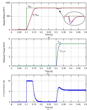
Fig. 8 shows a simulation result of the performance of the observer in the estimation of the torque and speed. At t = 0.1 s it is imposed a reference step speed of 800 rpm and t = 0.3 s the nominal torque is applied. From this result it is possible to verify that the observer is an agreement with the expected.
0 0 5 10 Time [s] 0 0.05 0.1 0.15 0.2 0.25 0.3 0.35 0.4 0.45 0.5 0 2 4 0 0.05 0.1 0.15 0.2 0.25 0.3 0.35 0.4 0.45 0.5 0 500 1000 Time [s] Time [s] 0 0.05 0.1 0.15 0.2 0.25 0.3 0.35 0.4 0.45 0.5 6 Nref N, Nest Text Text_est a) b) c)
Fig. 8. Simulation results of performance observer: a) Speed motor, b) External torque, c) Current motor.
IV. GENERAL CONTROLLER MODEL
This model is composed by three main blocks, namely: electric differential controller, speed and external torque observer and speed controllers,fig.9.
This model has as four inputs: (i) the speed reference (accelerator position), (ii) steering angle (iii) current and voltage motor values, and real velocity of the vehicle. The torque reference (Tm_ref), will be the reference for both independent
torque controllers; current (ia1, ia2) and voltage motor values
(ua1,ua2) from each drive wheel are used to estimate speed
wheels and external torque [12].
Fig. 10 presents the electric motor drive system proposed control for the electric differential.
Fig. 10. Electric differential for two independent wheel control model.
V. SIMULATION RESULTS
In order to verify the performance of the system, several simulation tests have been made. In these tests it was used a permanent magnet DC motor with parameters presented in appendix.
Fig. 11 shows a simulation result of the performance of the electric differential. Figs. 11 a) and b) presents the evolution of the speed and current in both motors for the steering angle variation.
Fig. 11. Simulation results: a) Speed wheels, b) Current motors.
Fig. 12 shows the simulation result of the performance of the electric differential. The evolution of the speed of each motor for the steering angle variation during 1.7 < t < 3.2 s (turn to right) is presented in figure 12 a). On other hand, fig. 12 b) shows the evolution of the electrical current in each motor and fig. 12 c) shows the trajectory vehicle.
0 5 10 15 20 25 -2 -1 1 2 X [m] 0 0.5 1 1.5 2 2.5 3 3.5 4 4.5 5 0 5 10 0 0.5 1 1.5 2 2.5 3 3.5 4 4.5 5 0 500 1000 0 Time [s] Time [s] N1 N2 I1 I2 a) b) c)
Fig. 12. Simulation results: a) Speed wheels, b) Current motors, c) Trajectory. Fig. 13 shows the simulation result for turn to right (1 < t < 3 s) followed turn to left (3 < t < 4 s). The evolution of the speed of each wheels drives, current motors and c) shows the trajectory vehicle are presented in figure 13 a).
0 5 15 25 30 40 -2 -1 1 2 X [m] 0 0.5 1 1.5 2 2.5 3 3.5 4 4.5 5 0 5 10 0 0.5 1 1.5 2 2.5 3 3.5 4 4.5 5 0 500 1000 0 Time [s] Time [s] N1 N2 I1 10 20 35 I2 a) b) c) N2 N1 I2 I1
VI. CONCLUSION
In this paper, a sensorless electric differential for two independent wheel drive EV was presented. The proposed electric differential algorithm allows to assure a trajectory in accordance with the steering angle. The vehicle dynamic model and tire model was also presented. The motor speed was estimated through speed and torque observers. In order to verify the proposed strategy, several simulations results were presented. From these results it was possible to confirm that the electric differential presents a good dynamic performance.
APPENDIX DCMOTOR PARAMETERS Nominal power 2500 W Nominal torque 5 Nm Speed 2100 rpm Armature Voltage 220 V Armature resistance 7.5 Ω Armature inductance 15 mH
EMF constant 0.971 Vs/rad Viscous friction 0.0006 Nms Moment of inertia 0.06 kgm2
ACKNOWLEDGMENT
This work was supported by national funds through FCT – Fundação para a Ciência e a Tecnologia, under project Pest-OE/EEI/LA0021/2013.
REFERENCES
[1] G. Maggetto, J. Van Mierlo, J, “Electric and electric hybrid vehicle technology: a survey” IEE Seminar Electric, Hibrid and fuel Cell Vehicles, 2000.
[2] Z. Q. Zhu, C. C. Chan, “Electrical Machine Topologies and Technologies for Electric, Hybrid, and Fuel Cell Vehicles” IEEE Vehicle Power and Propulsion Conference (VPPC08), pp. 1-6, 2008.
[3] N. Jinrui, W. Zhifu, R. Qinglian, “Simulation and Analysis of Performance of a Pure Electric Vehicle with a Super-capacitor” Vehicle Power and Propulsion Conference (VPPC06), pp. 1-6, 2006.
[4] Chen, Jialong ; Xu, Guoqing ; Xu, Kun ; Li, Weimin, “Traction control for electric vehicles: A novel control scheme”, 2012 International Conference on Information and Automation (ICIA), pp. 367-372, 2012.
[5] Jia-Sheng Hu ; Dejun Yin ; Hori, Y. ; Feng-Rung Hu, “Electric Vehicle Traction Control: A New MTTE Methodology “ IEEE Industry Applications Magazine,Vol. 18, pp. 23-31, 2012.
[6] J. Santiago, H. Bernhoff, B. Ekergård, S. Eriksson, S. Ferhatovic, R. Waters, M. Leijon, “Electrical Motor Drivelines in Commercial All-Electric Vehicles: A Review”, IEEE Transactions on Vehicular Technology, Vol. 61, No. 2, 2012.
[7] Chih-Hsien Yu, Chyuan-Yaw Tseng, Yuan-Sheng Hsu, “Electronic stability control for direct-drive Electric Vehicle”, International Conference
Electric Information and Control Engineering (ICEICE), pp. 4987-4991, 2011.
[8] Yongli Zhao, Yuhong Zhang , Yane Zhao, “Stability Control System for Four-in-Wheel-Motor Drive Electric Vehicle”, Sixth International Conference on Fuzzy Systems and Knowledge Discovery, vol.4, pp. 171 – 175, 2009.
[9] G. Genta, Motor Vehicle Dynamics – Modeling and Simulation. World Scientific Publishing Co, 1997.
[10] T. Gillespie, Fundamentals of Vehicle Dynamics. SAE – Society of Automotive Engineers, 1992.
[11] Arnet, B.; Jufer, M.: Torque control on electric vehicles with separate wheel drives, Proceedings of EPE’97, vol. 4, pp. 659-664, September 1997. [12] D. Foito, J.Maia, J Esteves, “Electric Differential and Regenerative Braking EV”, The 8th Mechatronics Forum International Conference 2002, 6-8 June 2002.
[13] A. Haddoun, M. E. H. Benbouzid, D. Diallo, R. Abdessemed, J. Ghouili, K. Srairi, “Sliding Mode Control of EV Electric Differential System”, XVII International Conference on Electrical Machines, 2006.
[14] M. Guerreiro, D. Foito, A. Cordeiro “A Sensorless PMDC Motor Speed Controller with a Logical Overcurrent Protection” JPE - Journal of Power Industrial Electronics, vol. 13, no. 3, pp 381-389, May 2013.