Luís Miguel Pereira Domingues Alho

(1)

Setembro, 2014

Luís Miguel Pereira Domingues Alho

Licenciatura em Ciências de Engenharia Biomédica

Automated quantitative analysis of MCC-IMS spectra

Dissertação para obtenção do Grau de Mestre em Engenharia Biomédica

Orientador: Valentina Vassilenko, Professor Auxiliar, Faculdade de Ciências e Tecnologia da Universidade Nova de Lisboa

Co-Orientador: André Damas Mora, Professor Auxiliar, Faculdade de Ciências e Tecnologia da Universidade Nova de Lisboa

Júri:

Presidente: Doutora Carla

Maria Quintão Pereira

Arguente: Doutor Pedro

Manuel Cardoso Vieira

Vogais: Doutora

(2)

(3)

Automated quantitative analysis of acetone and isoprene of MCC-IMS spectra

(4)

(5)

I

Agradecimentos

Esta tese representa não só a conclusão de um trabalho mas também a conclusão de toda uma etapa da minha vida, assim gostaria de agradecer a várias pessoas que tornaram isto possível.

Aos meus orientadores, Valentina Vassilenko e André Mora, pela informação e conhecimento transmitido, assim como toda a paciência e dedicação que tiveram para comigo ao longo deste trabalho.

(6)

(7)

III

Abstract

Ion Mobility Spectrometry coupled with Multi Capillary Columns (MCC -IMS) is a fast analytical technique working at atmospheric pressure with high sensitivity and selectivity making it suitable for the analysis of complex biological matrices.

MCC-IMS analysis generates its information through a 3D spectrum with peaks, corresponding to each of the substances detected, providing quantitative and qualitative information. Sometimes peaks of different substances overlap, making the quantification of substances present in the biological matrices a difficult process.

In the present work we use peaks of isoprene and acetone as a model for this problem. These two volatile organic compounds (VOCs) that when detected by MCC-IMS produce two overlapping peaks. In this work it’s proposed an algorithm to identify and quantify these two peaks. This algorithm uses image processing techniques to treat the spectra and to detect the position of the peaks, and then fits the data to a custom model in order to separate the peaks. Once the peaks are separated it calculates the contribution of each peak to the data.

Keywords: Ion Mobility Spectrometry (IMS); Multicapillary columns (MCC); Image

(8)

(9)

V

Resumo

A espectroscopia de mobilidade iónica (IMS) acoplada a Colunas Multicapilares (MCC) é uma técnica analítica rápida, que funciona a pressão atmosférica, com alta sensibilidade e alta selectividade tornando-a ideal para a análise de matrizes biológicas de alta complexidade.

A MCC-IMS gera informação sobre a forma de um espectro 3D. Este espectro fornece informação qualitativa e quantitativa na forma de picos, correspondentes a cada substância. No entanto estes picos por vezes aparecem sobrepostos dificultando a sua quantificação.

Neste trabalho utilizamos os picos de isopreno e acetona como modelo para este problema. Estes dois compostos voláteis orgânicos quando detectados pela MCC-IMS geram dois picos que se sobrepõem. É proposto neste trabalho um algoritmo para quantificar estas duas substâncias. Este algoritmo utiliza técnicas de processamento de imagem para tratar os espectros e para detectar a posição dos picos. Após a detecção destes picos o algoritmo ajusta um modelo personalizado aos dados do espectro de maneira a se poder separar os picos. Uma vez separados os picos calcula a contribuição de cada pico no espectro.

Palavras-chave: Espectroscopia Mobilidade Iónica (IMS); Colunas Multicapilares

(10)

(11)

VII

Tables

Table 4.1 - Initial parameters of lognormal curve and their upper and bottom bounds ... 20

Table 4.2 - Initial parameters of lognormal curve and their upper and bottom bounds ... 20

Table 4.3 - Analysis of the empiric detection of acetone peak ... 22

Table 4.4 - Analysis of the empiric detection of isoprene peak ... 22

Table 4.5 - Analysis of the empiric region of interest ... 23

Table 4.6 - Initial parameters and their upper and lower bounds for the peaks model ... 27

Table 5.1 - Results of the acetone peak detection ... 29

Table 5.2 - Results of the isoprene peak detection ... 30

(14)

(15)

XI

Figures

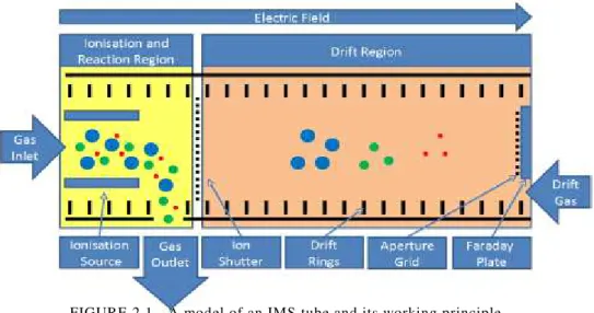
Figure 2.1 - A model of an IMS tube and its working principle ... 6

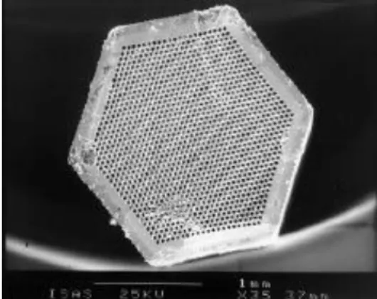
Figure 2.2 - A multi capillary column ... 7

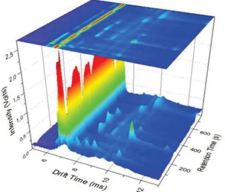
Figure 2.3 - Pseudo color representation of IMS data ... 8

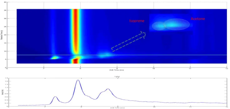
Figure 2.4 - ATopografic view of a MCC-IMS spectrum and a single spectrum line ... 9

Figure 2.5 - Example of a 2D fitting process to a MCC-IMS spectrum ... 10

Figure 3.1 - Before and after RIP detailing by subtracting the detailing function ... 13

Figure 4.1 - Results of different filters applied in a single line spectrum ... 18

Figure 4.2 - Result of the rip detailling ... 21

Figure 4.3 - Example of the region of interest selection ... 23

Figure 4.4 - Peak detection algorithm example ... 24

Figure 5.1 - Acetone peaks distribution ... 30

Figure 5.2 - Isoprene peaks distribution ... 31

Figure 5.3 - Result of the fit ... 32

Figure 5.4 - Acetone peak isolated ... 33

Figure 5.5 - Third peak isolated ... 34

Figure 5.6 - Isoprene peak isolated ... 34

(16)

(17)

XIII

Abbreviations

E Electric Field

GIM Growing Interval Merging GPL Gradient Path Labeling IMS Ion Mobility Spectrometry K Ion Mobility

K₀ Reduced Ion Mobility MCC Multicapillary Columns

MPCL Merged Peak Cluster Localization RIP Reactant Ion Peak

ROI Region Of Interest tDrift Drift Time

tRet Retention Time vd Ion Velocity

VOCs Volatile Organic Compounds

(18)

(19)

1

1. Introduction

Ion Mobility Spectrometry is a recent analytical technique for the detection of gas-phase analytes. Because its operation does not require vacuum, IMS is seen as one of the most promising techniques for gas spectrometry.

Developed during 1970’s it was initially used for military purposes [1]. Initially

seen as a niche technology, without much room for improvement, its development slowed down and the technique turned into a rejected method. This rejection occurred due to the lack of understanding of the principles of ion molecule chemistry and ion

behavior at atmospheric pressure. In the 90’s refinements in the IMS instrumentation

expanded the capabilities of the technique, becoming a general-purpose technology [2].

The coupling of IMS with multi capillary columns (MCC) increased the technique selectivity without resorting to pre-separation techniques.

This combination brought new possible applications for the technique, being the detection of volatile organic compounds (VOCs) one of the most interesting and promising applications. Volatile organic compounds are organic chemicals that possess low boiling point and so evaporate at ambient temperatures. These compounds have numerous origins, including biological and anthropogenic sources. VOC monitoring has numerous applications, some of them can be harmful to human health while others can be indicators of biological processes, like the detection of Dyacetyl in beer fermentation, quality control of food, and detection of marker substances in human breath [3]. Isoprene and acetone are two VOCs that, due to their characteristics, appear

in the IMS spectra in close positions and because they have some relevance in the metabolic profiling, medical diagnosis and therapy monitoring will be studied in this work.

Acetone ((CH3)2 CO) is an organic compound widely used as a solvent in the

industry. It has a molar mass of 58.08 g mol−1 and its boiling point is between 56ºC and

57ºC in standard conditions, making it a high volatile substance. In ambient conditions

(20)

2

of decaying apples” by John Gallo. More recent studies have found relationships between the concentrations of acetone in breath and diabetes (e.g. in human breath acetone at a concentration of 400 ppb is normal but at 1000-1200 ppb can be an

indicator for diabetes). Also correlations of the concentration of acetone in breath and exercise intensity have been found [4] [5].

Isoprene (C5H8) is another organic compound with a molar mass of 68.12 g

mol−1and its boiling point is 34ºC in standard conditions. Possesses high volatility and

it’s produced by all kinds of living organisms, including human beings. Like Acetone, it’s always present in the human breath and variations of its concentration levels can be

used as an indicator of health and disease. Although no conclusive results have been taken isoprene levels are believed to be a good additional indicator to metabolic disorders and also in cancer screening [6] [7] [8].

The MCC-IMS spectrum is a 3D matrix that contains the information of the detected substances as peaks. The position of these peaks in the spectrum gives qualitative information of the detected substances. Resorting to automatic methods to detect peaks and, subsequently, using statistical analysis, correlation between a peak position and what substance it represents can be achieved. There is also the possibility to extract quantitative information from these peaks.

(21)

3

1.1. Outline

This thesis is organized in 6 main chapters. Chapter 1 is the introduction, where

the theme of this thesis is introduced. Chapter 2 is comprised of the IMS-MCC details,

giving an idea of the physical background, the resulting data and its associated problems. In Chapter 3 the current state of art techniques used in the IMS-MCC data

are presented. In Chapter 4 all the methods used in this work are explained as well as

the justifications of the choices made throughout the work. Chapter 5 contains the

analysis of the data obtained as result of this work. Chapter 6 is where the final

conclusions of this work are made and proposals of future work are given. This work also has two appendixes. Appendix A contains a series of results achieved with the

algorithm presented in this thesis. Appendix B contains the poster accepted and

exposed in the 8th International Conference on Breath Research & Cancer Diagnosis.

(22)

(23)

5

2. Theory

2.1. Ion Mobility Spectrometry

2.1.1. Working Principles

IMS is based on a simple principle, ions created at normal pressure move in the direction established by an external electrical field against the direction of a carrier gas. IMS ionizes gaseous analytes and then extracts the information of their characteristic drift time. The ions drift time is characteristic because their mass and/or structure make them attain different velocities in the drift gas [9] [10]. Due to the relation between the

ion velocity and the intensity of an applied external electric field an independent component for each ion can be extracted. This component is the quotient between ion velocity ( ) and Electric field ( ) and is referred as ion mobility ( ).

2.1

Ion velocity is expressed in and the electric field is in therefor the ion mobility is expressed in . Due to the physical laws of our universe, ion mobility is susceptible to both temperature and pressure. This susceptibility required a correction in order assure stable results. By normalizing to the standard temperature and pressure we get the reduced ion mobility ( ).

( ) ( )

2.2

(24)

6

An ion mobility spectrometer is comprised of a series of components. Usually the spectrometer main components are a drift tube, a sample inlet, a high voltage supply, a shutter grid, an amplifier, a drift gas supply, pressure and temperature sensors, and a computer.

The drift tube is the main component of the spectrometer. Two entrances (the inlet sample and the drift air entrance), an exhaust exit, a Faraday detector, a shutter grid, a radiation source, drift rings and an aperture grid are the elements present in the tube. Divided by the shutter grid two regions exist, the ionization region and the drift region.

In the ionization region the radiation source forms positive and negative ions. Because these ions are reactant the sample molecules undergo ion molecules reactions forming product ions. Opening the shutter grid for a moment allows the product ions to get into the drift region. An electric field is applied on the product ions. These ions migrate against the drift gas due to the electric field. Since the ions possess different masses and/ or structure, they reach the Faraday plate at different times. The different signals generated by the detector are recorded in the ion mobility spectrum, giving information on the different drift times (ms) and their respective intensity.

2.1.2. Spectrometer Components

The tube is usually made of metal rings separated by isolators. The high-voltage supply (±1-10 kV) creates an electric field inside the tube with field gradients from 150

to 300 V/cm. Their design depends on the ionization source selected. Presently the know

(25)

7

sources for IMS include radiation sources (α and β radiation), UV lamps, lasers,

different kinds of discharges, and electrospray ionization [2]. The most common β

radiation source is 63Ni although Tritium can also be used for some applications.

The shutter grid works by creating an additional field gradient that is perpendicular to the one of the measuring tube not allowing the ions to pass. When the field is turned off the ions can pass through the grid.

For the purpose of getting better mobility spectra an aperture grid is positioned in front of the detector. It provides a capacitive decoupling between arriving ions and the detector resulting in a mall line width of the peaks in the spectra.

2.2. Multi Capillary Columns Coupling

Multi capillary columns consist of various capillaries (around 1000) all bundled into a single tube with a typical diameter of 3 mm. Their function is to separate complex

mixtures, while offering high flow rate and a high sample capacity when compared to single narrow bow columns [11].

Because the ion mobility spectrometer does not have a very high selectivity, there is the need to be coupled with MCC. MCC offers a high carrier gas flow which enables an isothermal separation of VOCs at ambient temperatures. Thus, because of the high capacity, favorable flow conditions, and low working temperatures, MCC is ideal to be coupled with IMS, assuring that the equipment does not have to increase in size.

(26)

8

The IMS-MCC coupling also enables a multidimensional data analysis, allowing identification of VOCs by both chromatographic data (retention times) and by the ion mobility data. The multidimensional data analysis also allows the distinction of monomers, dimers and trimmers of certain molecules.

2.3. Spectrum

The spectrum generated by the IMS-MCC spectrometer is a 3 dimensional plot.

The drift time is in the x-axis, the retention time is in the y-axis, and the intensity of the signal from the Faraday plate is in the z-axis. This data can be plotted in topographic view with the intensity being color-coded, which allows easy pattern detection, crucial for the detection of VOCs.

An IMS spectrum has one characteristic peak that appears in all spectra. It’s

called the reactant ion peak (RIP) and its descent signal is called the RIP tailing. The RIP is formed by the ionization of the carrier drift gas. If there are no molecules detected the RIP has the maximum amount of ions, this means that in zone where a

(27)

9

molecule is detected the RIP decreases in size. This phenomenon occurs because the product ions of the sample molecules are made by the collisions of reactant ions and sample molecules [2].

Each substance has a specific peak due to its reduced ion mobility constant. However, when multiple substances are analyzed, some peaks can overlap. When peaks are overlapped they give cumulative contributions to the spectrum. For a precise quantification of substances peaks the different contributions need to be isolated.

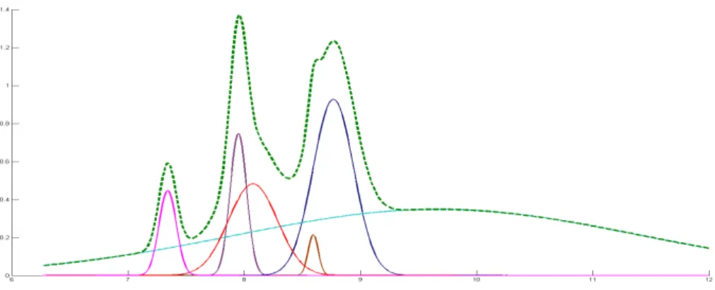
Figure 2.4 is an example of a simple IMS spectrum. It will be used to explain the profile of a peak and its characteristics.

First the peaks need to be characterized A process of fitting is to be applied to modulate these peaks. This process allows an easier analysis of the complexities of the spectrum. After the identification of the individual peaks’ characteristics, a correlation between these characteristics and the concentration of substance can be achieved.

Figure 2.4 is an example of two overlapped peaks (Isoprene and Acetone). Using a side view we can observe the peaks profile, allowing a better understanding of what shape each peak has. The peaks seem to exhibit the shape of a Gaussian curve with a tailing in the direction of the drift time. They are also standing on top of a baseline

curve. To isolate the “real” values of the peaks, they need to be isolated. First the peaks

need to be characterized and a model created. Then a process of fitting is to be applied

Acetone Isoprene

(28)

10

to find the parameters that best represent the data in the model. This process allows for an easier analysis of the complexities of the spectrum their corresponding contributions. After the identification of the individual characteristics of peaks, a correlation between these characteristics and the concentration of substance can be achieved.

(29)

11

3. State of Art of Spectra Analysis

In the scope of quantitative analysis of IMS spectra, this section presents the current techniques for IMS spectra data analysis. These methods provide the necessary tools to treat the data in a way that the peaks deconvolution can be achieved.

3.1. De-noising and Smoothing

Like most spectra, MCC-IMS spectra contains noise. This noise makes it difficult to detect low intensity signals. The process of de-noising and smoothing the data allows the reduction or the enhancement of certain aspects of the data. However this process can lead to loss of crucial information. This means that there is the need to find a filter that produces negligible loss of information and still maintain the important aspects of the data. The characteristics of the noise and the data influence the choice of the filter. The following sections present some filtering techniques.

3.1.1. Moving Average Filter

The Moving average filter is a filter that evaluates the average value on a determined window focused on each point of a data set. Although it is very fast filter to compute, it does not distinguish data and noise very effectively, leading to strong attenuations of the data and loss of important information.

3.1.2. Savitzky-Golay Filter

The Savitzky-Golay filter is a digital filter proposed by Savitzky et al. in 1964 [12]. The filter possesses 2 adjustable parameters, the window size and the polynomial

(30)

12

height of waveform peaks [13]. The filter works by splitting the data in samples

(window size determines the size of this samples) then a linear regression of some polynomial individually for each sample, followed by the evaluation of that polynomial exactly at the very position of the sample [14].

3.1.3. State of Art

Wavelet transforms were used by Bader et al. 2008 [15]. Applied to different

levels of resolutions these wavelet transforms achieved both de-noising and smoothing. Removing low amplitude coefficients resulted in de-noising. Removing the coefficients corresponding to high frequency regions resulted in smoothing of the data.

Bunkowski used a combination of filters to achieve de-noising [16]. A median

filter followed by a Gaussian filter. The median filter is used to eliminate single noise fragments and the Gaussian filter to smooth the remaining values.

3.2. Curve Fitting

Curve Fitting is the process of finding a curve that best fits a certain data set. This curve or mathematical equation allows for a better visualization and a better analysis of the data. Two things are needed for this process, a model that can describe the data and a method that can find the ideal parameters for the model. The fitting process can require a lot of computation time, depending on the size of the data and the number of parameters that needs to calculate.

(31)

13

Gauss-Newton method it possesses the ability to create boundaries to the parameters that solved the non-linear regression problem.

3.3. RIP detailing

A characteristic signal structure is found in all MCC-IMS spectra, the reactant ion peak (RIP). To facilitate analysis there is the need to eliminate this peak. This process is called RIP detailing.

In 2008 Bader et al. achieved RIP detailing by fitting a modified lognormal

function (3.1), where θ is the shift in the x axis, σ defines the shape of the curve, and μ is the log scale, to the mean of all spectra and then subtracting the fitted function from each spectrum [15].

(

)

₍ _{) √}

*

[ (( ) )]

+

3.1

This lognormal function met the general assumption of Gaussian peaks and the right screwed shape of the RIP tailing.

More recently, Bunkowski proposed a method where an ascending sorted list with all the values with the same 1/K0 value is created [16]. Then, the 25% quantile of

every 1/K0 is selected and subtracted over all spectra. This method removes the RIP and corrects the baseline.

(32)

14

3.4. Peak Detection

Both Bader and Bunkowski presented different approaches to detect peaks in IMS data. Bader introduced three different methods, the Merged Peak Cluster Localization (MPCL), the Growing Interval Merging (GIM), and the Wavelet-Based Multiscale Peak Detection (WBMPD) [15]. Bunkowski introduced an algorithm based

on Watershed Transformations (WST) [16].

3.4.1. Merged Peak Cluster Localization

This method instead of utilizing a preprocessing baseline correction, it uses a LOWESS algorithm [17]. LOWESS is a robust locally weighted regression method that

was used to reduce the RIP tailing and mitigate the signal noise. After the LOWESS algorithm is applied the data is the data is truncated after the RIP. This truncated data is then classified into two types, peaks and noise by k-means clustering. Finally a merging algorithm is applied to group the adjacent data points that were classified as peaks. Although some positive results were achieved, an important limitation of the method is its inability to detect superimposed peaks.

3.4.2. Growing Interval Merging

This method was developed to overcome the limitations of the MPCL method [15]. It starts by defining a sequence of intensity thresholds that characterize the

(33)

15

manner. In each stage a list is created with the peaks detected. If in the next stage a common peak is found the old peak parameters are overridden by the new parameters. Although the GIM outperforms the MPCL, there are still limitations in the detection off overlapping peaks.

3.4.3. Wavelet-Based Multiscale Peak Detection

This method is based on the approach by Randolph and Yasui for multiscale processing of single spectra [18] but applied to three-dimensional spectra. A maximal

overlap discrete wavelet transform (MODWT) to perform multiple resolution analysis is used. This wavelet transform is translation invariant and can be applied to arbitrary data dimensions. A Haar wavelet yield better results. The wavelet transform produces four matrices with information of the data, the lowpass-lowpass (LL), the lowpass-highpass (LH), the highpass-highpass (HH), and the highpass-lowpass (HL). For the IMS data the LH matrices provided the necessary information for peak localization. Bader et al.

applied the GIM method to the LH matrix to detect the peaks and extract their information. This method proved to be highly sensitive and provided better results than the standalone GIM method.

3.4.4. Watershed Transformation

Bunkowski proposed this method based on the work of Wegner et al. for the detection of spots in gel electrophoresis images. The concept of WST is by analyzing

the data as a topological permeable map which is submerged into an imaginary water

basin [16]. The IMS data is inverted so that the peaks reach the water first. The water

(34)

16

3.5. Peak Modeling

Kopcynski, Baumbach and Rahmann proposed a model for the IMS peaks [19].

This model is an inverse Gaussian distribution. While the original inverse Gaussian has its origin at zero the proposed model has an additional offset parameter, this means a

total of three parameters are needed. Although there is no physical theory to describe the peaks observed this model possesses similar characteristics to the observed peaks. The ability to represent the data in a mathematical model and a series of parameters for each peak requires less space than saving millions of data points.

(35)

17

RIP Detailling Spectral Peaks Detection

Spectral Peaks Modelling

Metabolites Quantification RIP Detailling Spectral Peaks

Detection Spectral Peaks Modelling Metabolites Quantification

4. Methods

4.1. Process

In order to extract the quantitative information of Isoprene and Acetone peaks from the IMS spectra data, a methodology had to be applied.

To reduce noise and fix data irregularities, a filter is applied in order to enhance the aspects of interest and improve the ensuing methods of the algorithm. Then, the RIP tailing is detected using 2D fitting and then subtracted, followed by the segmentation algorithm (described later on) applied in a specific area in order to detect the number of peaks and its position. Once the necessary information is collected a 3D fitting using the defined peak model is applied to achieve a representation of the data can be used to deconvolute the peaks and allow their quantification.

4.2. Data Filtering

The first step in the methodology was to apply a smoothing filter to reduce the noise influence. The filter was chosen considering the MCC-IMS spectra data, i.e. containing overlapping peaks.The filter had to be able to reduce the noise without significant changes to the shape of the peak curves.

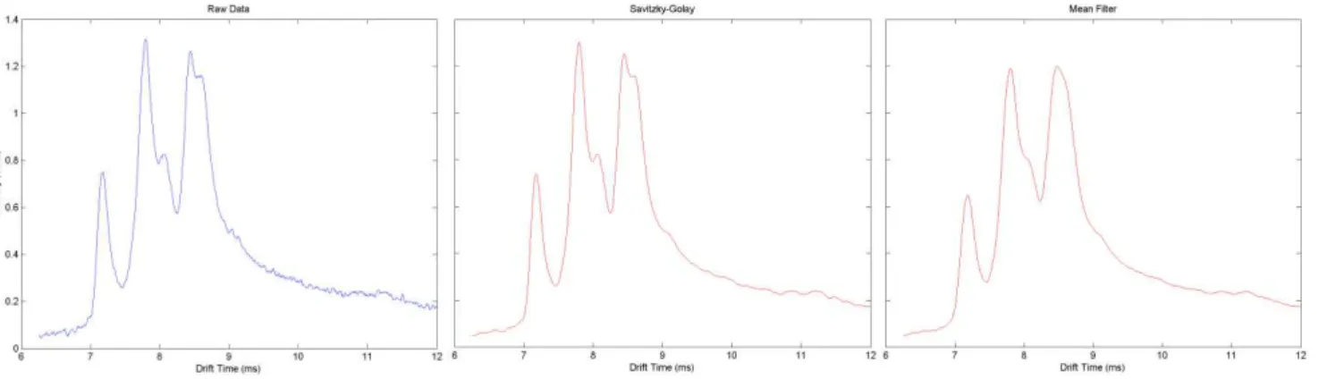
The Savitzky-Golay filter is the filter widely used in the literature and in the industry, with proven results in this type of data. This filter efficiently removes de noise without changing the peaks’ shape. In this work Savitzky-Golay filter was applied using the MATLAB® function sgolayfilt to each retention time spectra. A 13 pixel window

(36)

18

In figure 4.1 it can be clearly seen that the Savitzky-Golay filter reduces the noise in the data without changing the curve shapes like it happens in a moving average filter.

4.3. RIP Detailing

In order to facilitate the quantitative analysis of IMS the RIP tailing had to be described in a mathematical formula and then proceed to its removal. The IMS RIP has incremental contributions to the value of the peaks. To quantify the peaks, these contributions need to be found and removed. Based on the work of Bader et al. a lognormal equation was used to describe the RIP tail [15]. This lognormal equation in

based on the lognormal statistical distribution. The calculation of the equation parameters required a series of steps as well as observation of the equation behavior in order to create reasonable bounds to those parameters.

The first step was to calculate the second derivative of the curve in order to find the major peaks. Then the Savitzky-Golay filter is applied to the second derivative result in order to facilitate the use of the findpeaks function of MATLAB®. The

findpeaks function was sed to find the peaks that have at least 20% of the max value of

the spectra and a minimum distance of 15 pixels between peaks. The position and the value of these peaks are then extracted to a data structure.

(37)

19

The second step uses the information saved in the data structure to create an estimation model. The number of peaks found decides the number of Inverse Gaussian Distribution curves it creates. The Inverse Gaussian distribution is an exponential

distribution with 2 parameters, μ and λ.

Where μ < 0 is the mean and λ < 0 the shape. Its probability density function is given by the equation 4.1 and it’s characterized by having a single peak and by not being

symmetric, having a right tail. The position of the single peak is given by the mode. The

mode depends on both parameters (μ, λ) and is given by [( ) ]. For the modeling of a single curve two extra parameters were added. An intensity parameter that allows the curve to better adapt to the data and an offset x0 that represents position where the curve starts.

The model consists in the major peaks, found with the second derivative and modeled with the Inverse Gaussian distribution curve, plus the lognormal function for the RIP tail. A function type file receives two structures, the drift time vector (tDrift) and a structure (GParameters) with all the parameters necessary to create the mathematical model.

The third step uses the Levenberg-Marquardt algorithm to find the ideal parameters for the model created. In order to apply the Levenberg-Marquardt algorithm we use the lscurvefit function of MATLAB®. This function receives the estimation

model we want to use, a structure with the initial parameters, the values of the raw data, the tDrift, and two structures with the maximum and minimum bounds for the parameters.

The parameters bounds were added through the observation of the behavior of the curve. For the lognormal curve to best represent the RIP tail its behavior had to be controlled using a set of bounds within the Levenberg-Marquardt algorithm. These bounds are specific to the type of spectra used in this work. They ultimately limit the values found by the Levenberg-Marquardt algorithm, which means the values found

(38)

20

may not be the most optional values in terms of the minimum value found by the error function but are the values that best represent the data.

Once the all parameters are found, they are introduced in the model function and the data representation is created. For the detailing of the RIP, only the parameters of the lognormal function are used.

The RIP detailing was tested in two different ways. In one the model fitting was applied to all the spectral lines and then the mean log normal curve was calculated. In the other way the mean spectrum was calculated and then the model fitting was applied to the mean spectrum.

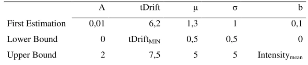
The process where the fitting was applied to all the spectral lines produced good results but its time consumption was really high. The application of Levenberg-Marquardt algorithm in each line requires a really high processing power. Assuming that the model in average possesses 3 inverse Gaussian curves (4 parameters) and a lognormal curve (5 parameters), the algorithm had to calculate the optimal value of 17 parameters for each line. Even though this process produces more consistent results, the differences in results did not compensate the time spent. This process also had a different set of bounds of the lognormal curve then the other process, in table 4.1 the parameters used in this process is presented.

Table 4.1 - Initial parameters of lognormal curve and their upper and bottom bounds

A tDrift μ σ b

First Estimation 0,01 6,2 1,3 1 0,1

Lower Bound 0 tDriftMIN 0,5 0,5 0

Upper Bound 2 8 1,3 2 Intensitymean

Calculating the mean spectrum along the retention time and then fit the model to this new data resulted in a faster process, mainly because the Levenberg-Marquardt algorithm runs a single time. In order for this method to work with acceptable results it required some customizations.

Table 4.2 - Initial parameters of lognormal curve and their upper and bottom bounds

A tDrift μ σ b

First Estimation 0,01 6,2 1,3 1 0,1

Lower Bound 0 tDriftMIN 0,5 0,5 0

(39)

21

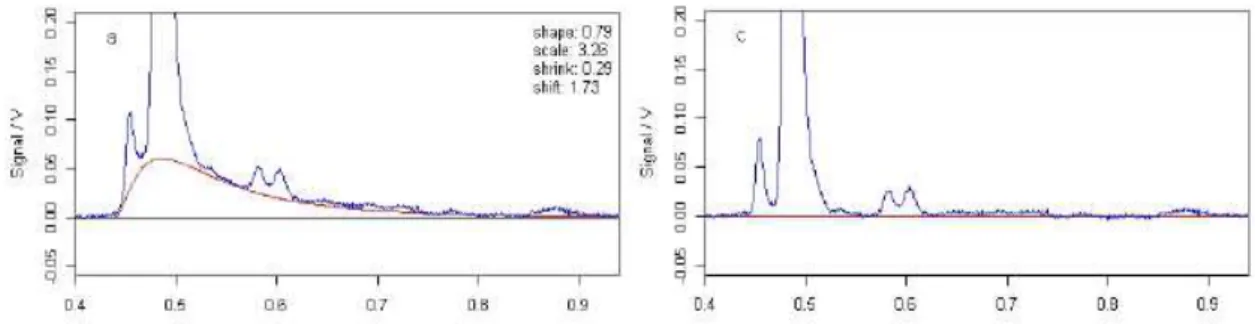
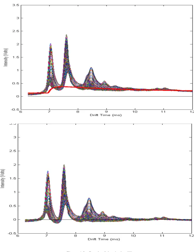
The lognormal curve has a different set of bounds (table 4.2) and the process of finding peaks is wider in terms of the number of peaks it can find. This means that the model can find more curves, being more precise describing the mean spectrum. In figure 4.2 we can see an example of the RIP detailing. On the left is the result of the detailing and on the right is the plot of all the spectrum and the RIP tail curve that was calculated with the method developed.

(40)

22

4.4. Region of Interest

To find the correct position of the Acetone and Isoprene peaks it was necessary to find the region of interest in which the peaks were to be found using the spectral peak detection tool. This region of interest was found using several spectra that contained acetone and isoprene peaks.

Table 4.3 - Analysis of the empiric detection of acetone peak

Acetone Peak

tDrift (ms) tRet (s)

Average 8,543 8,737

Standard Deviation 0,056 0,908

Maximum Values 8,653 9,828

Minimum Values 8,440 6,174

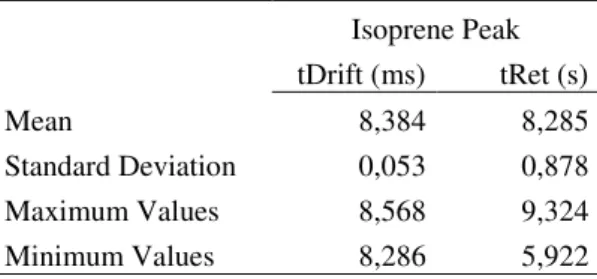
In table 4.3 and 4.4 the positions of the acetone and isoprene peaks extracted empirically are presented. It can be seen that the position of the acetone peak is very contained in the tDrift axis, with its average value being 8,543ms and with a standard deviation of 0,056ms, indicating that the value does not deviates much from its average value. On the other hand the position on the tRet axis has a wider range with the average value being at 8,737s with a standard deviation of 0,908s. This wider range is justified by some peaks reaching a maximum of 9,828s (~+1) and a minimum of 6,174s (~+2), indicating some considerable fluctuation in the tRet.

Table 4.4 - Analysis of the empiric detection of isoprene peak

Isoprene Peak

tDrift (ms) tRet (s)

Mean 8,384 8,285

Standard Deviation 0,053 0,878

Maximum Values 8,568 9,324

Minimum Values 8,286 5,922

(41)

23

Table 4.5 - Analysis of the empiric region of interest

Region

Average Standard Deviation Maximum Minimum

Bottom tDrift (ms) 8,22961 0,05651 8,38600 8,14000

Top tDrift (ms) 8,75627 0,07078 8,98000 8,58600

Bottom tRet (ms) 6,90348 0,69106 8,06400 5,16600

Top tRet (ms) 11,77109 1,35701 16,51000 9,07200

Surface (ms2₎ _2,59745 _0,84202 _6,55829 _1,60149

Dif tDrift (ms) 0,52666 0,05738 0,75400 0,39300

Dif tRet (ms) 4,86761 1,10720 9,07600 2,89600

Table 4.5 gives the information of the region that contains the peaks. The region contains the relevant area to correctly quantify the peaks. Once more the range in the tDrift axis does not vary much, which correlates to the fact that the Drift time is related to the ionic mobility of the substances. Using this information the region of interest was

defined as μ+2σ to the top values of tDrift and tRet and as μ-2σ to the bottom values of

tDrift and tRet. This resulted in a region with a top corner situated at (8,8978ms ; 14,4851s) and a bottom corner situated at (8,1166ms ; 5,5214s).

(42)

24

In figure 9 we have two examples of the region of interest implemented in the algorithm. The region chosen has the necessary information for the peak detection and fitting.

4.5. Spectral peak detection

For the spectral peak detection the gradient path labeling algorithm (GPL) was used [20]. GPL detects the regional maximums in the region of interest chosen earlier.

Because a gradient image have a confluence of several ascending paths towards a regional maximum, GPL is a method of segmentation based on the labeling of these gradient paths. The algorithm is divided in two stages.

The first stage starts by attributing a label to each pixel of the image in a top-left to bottom-right direction and determining its gradient azimuth using a 3x3 Sobel operator.

Once all the pixels are labeled the algorithm propagates the labels following the gradient path until an already marked or outside image boundaries pixel is found. When the propagation finishes on a different label, the two labels are tagged as equivalents

and considered to belong to the same maximum.

(43)

25

The second stage of the algorithm is when the equivalences are applied and the

image is segmented and each segment is a maximum or, in the context of this work, is a peak.

Due the shape of the curves, not all gradient paths end on the same maximum pixel, resulting in over-segmentation of the image. Although a merging method exists in the GPL algorithm, it was not sensitive enough to correctly detect the peaks. In order to extract the correct position of the isoprene and acetone peaks, the regional maximums detected by the GPL are posteriorly filtered. The filter applied has 3 steps and is based in the empiric observation of various spectra presented in the region of interest chapter (5.4). First the method checks if any peaks are present in an area with one standard deviation of uncertainty around the average value of the peaks. If no peaks are found the method passes to the second step, this one is basically equal to the first but widens up the area to two standard deviations on uncertainty. If more than one peak is found, the method picks the one with the highest intensity.

4.6. Spectral peaks modeling

The substance peaks in the IMS spectra, at first sight, look like they can be described by a Gaussian curve, but the elongations in tDrift and tRet discredit the first observation. Based on the work of Kopcynski, Baumbach, and Rahmann and the

observation of various spectra the Inverse Gaussian Distribution curve was found to be the equation that could be used to describe the peaks with the elongations [19].

To develop the 3D model that describes the IMS peaks, two Inverse Gaussian Distribution curves were multiplied, one representing the tRet axis and another the tDrift axis. The curves also had some changes to the original equation in order to be able to adapt to the IMS data. These changes consisted in adding two new parameters, the intensity (Ax,Ay) and the position of the beginning of the curves (x0, y0). In the final

f( y)

r y y

𝐴 √ _𝜋₍_𝑥𝜆𝑥_𝑥 ₎ 𝑒𝑥𝑝[ 𝜆𝑥((_𝜇𝑥 𝑥) 𝜇𝑥)

𝑥 (𝑥 𝑥) ] √

𝜆𝑦

𝜋( 𝑦 𝑦) 𝑒𝑥𝑝

𝜆𝑦((𝑦 𝑦) 𝜇𝑦)

(44)

26

model a single parameter for the intensity (A) appears due to the multiplication of Ax and Ay, the reduction of the parameters number simplifies and reduces the number of calculations needed to find the optimal value.

During the peak location stage, the algorithm finds the position of the peaks however the model uses the position of the start of the curve making it necessary the calculation of the position of the peak related to the start of the curve. This is achieved using the mode of each curve. The mode gives the position of the maximum value relatively to the start of the curve. Using this information the position of the peak in tRet and tDrift is given by and .

The Levenberg-Marquardt algorithm is used to find the parameters that allow the model to best adapt to the data, resorting once again in the MATLAB® lscurvefit

function. The lscurvefit function receives the region of interest data, a structure

containing both the tDrift and tRet vectors of the region of interest in grid form, a structure with all the initial parameters to the model, and two structures with the top and low bounds for the parameters.

The tDrift and tRet vector were transformed into matrices using the meshgrid

function of MATLAB®, this step was a necessity due to the characteristics of lscurvefit,

because as the name implies it’s a function for curves and not surfaces, this was circumvented using a single structure with both vectors as grids. The other reason this method works is because once the data enters the function, the Levenberg-Marquardt

algorithm does not care it it’s a curve or a surface and resolves the non-linear problem presented.

The initial parameters are generic values for the peak shape and the positions detected by the GPL for the peak location. The Levenberg-Marquardt algorithm receives the parameters for the number of peaks detected plus one additional peak. This additional peak helps the algorithm to shape the model to the best fit possible, it also tries to stop the algorithm to try to compensate noise structures with the peaks.

(45)

27

Table 4.6 - Initial parameters and their upper and lower bounds for the peaks model

A tDrift tRet

x0 λ μ y0 λ μ

Estimation GPL GPL 1 1 GPL 1 1

Lower Bound 0 GPL - 0,05 0,5 0,1 GPL - 0,9 0,5 0,1

Upper Bound 10 GPL + 0,05 100 10 GPL + 0,9 100 10

With the parameters found, seven for each peak, a recreation of the data is produced that can be used for comparison with the data. To evaluate the goodness of the fit it is possible to calculate the total volume of both images and compare the values. It is also possible to calculate the mean squared error between each pixel of the image.

(46)

(47)

29

5. Results of Peak Analysis

For data analysis there are two main indicators being evaluated, the automatic detection of the peaks and the goodness of the fit. These two indicators are the ones that best assess the quality of the algorithm. Good automatic peak detection is essential for future works and has multiple applications. The goodness of the fit can be used to validate if the chosen method and model are correct to quantify substances in MCC-IMS spectra.

5.1. Peak Detection

To give an overview of the results produced by the GPL algorithm the same spectra empirically analyzed were analyzed by the algorithm and a comparison of the results is presented here. A total of 77 spectra with isoprene and acetone peaks were analyzed. The average value of the peaks and its respective standard deviation will be analyzed as well as the differences in the position of the peaks in each spectrum.

5.1.1. Acetone Peak

In the spectra analyzed the acetone peak is usually the most intense. As it was referred before, it is located around the point (8,543ms; 8,737s). In table 5.1 is given an overview of the differences between the empiric detection and the automated detection. The differences in value of the mean value and the standard deviation are small, what may indicate a good behavior of the algorithm, although not enough to formulate a conclusion.

Table 5.1 - Results of the acetone peak detection

Acetone Peak

Empiric GPL Difference

tDrift (ms) tRet (s) tDrift (ms) tRet (s) tDrift (ms) tRet (s)

Mean 8,54261 8,73677 8,51618 8,59091 0,02643 0,14586

(48)

30

In order to get a better overview of the GPL algorithm’s behavior, in figure 5.1 the multiple acetone peaks detected, empirically and by the algorithm, are presented.

Here it’s displayed the position of the mean value for each detection method, with error

bars representing two standard deviation of uncertainty. It can be noticed that the peak positions follow a similar distribution. The average error between peaks detected by both methods is 0,50% in the tDrif axis and 6,89% in the tRet axis, although in some cases in the tRet axis the error is up to 60,78%. According to these values, it can ve concluded that the acetone peak is being correctly detected by the algorithm.

5.1.2. Isoprene Peak

In the analyzed spectra the isoprene peak is not always present and is usually less intense than the acetone peak.

Isoprene Peak

Empiric GPL Difference

tDrift (ms) tRet (s) tDrift (ms) tRet (s) tDrift (ms) tRet (s)

Mean 8,38416 8,28520 8,37467 7,73951 0,00949 0,64465

Standard Deviation 0,05248 0,87764 0,05918 0,98086 0,00670 0,10322 6 6,5 7 7,5 8 8,5 9 9,5 10 10,5 11

8,4 8,45 8,5 8,55 8,6 8,65 8,7

TRe

t

(s)

tDrift (ms)

Acetone peak distribution

Empiric

Empiric Average

GPL

GPL Average

Figure 5.1 - Acetone peaks distribution

(49)

31

In table 5.2 it can be seen that the differences in the tDrift values are minimal and in the tRet, although bigger than the differences in tDrift, are small enough to get a good overview in the quality of the detection.

In figure 11 the distribution of the peaks is represented, once again with the position average value and its respective error bars with a two standard deviation uncertainty. The behavior of the algorithm when detecting the isoprene peak is also very good. With an average error of 0,48% in the tDrift axis and 8,67% in the tRet axis, and a maximum error of 2,43% in the tDrift axis and 44,68% in the tRet axis. It can be concluded that the algorithm detects the correct position of the isoprene peak. It is also worth to mention that some isoprene peaks were not detected by the algorithm. There are two reasons for this. In some spectra the acetone peak was so intense that masked the isoprene peak. While in other spectra the isoprene peak was so small that the

algorithm ignored it because it didn’t have enough intensity. 5,5 6 6,5 7 7,5 8 8,5 9 9,5 10 10,5

8,2 8,25 8,3 8,35 8,4 8,45 8,5 8,55 8,6

Isoprene Peak Distribution

Empiric

Average Empiric

GPL

Average GPL

(50)

32

5.2. Fit

To have a perception of the goodness of the fit first the analysis will focus in a single spectrum and then a statistical overview of a series of tests will be presented.

This spectrum went through the whole process algorithm and the results are

going to be discussed.

Figure 5.3 is presents the result of the fit. It can be observed the presence of 3 peaks. At first sight the main difference is how smooth the fit is. In the treated data the position of the acetone peak, found by the detection method, was 8,500ms in tDrift and 7,938s in tRet and in the fit its position is 8,493ms in tDrift and 9,938s in tRet. As for the isoprene peak the detection method determined its position was 8,313ms in tDrift and 7,308s in tRet and in the fit its position was 8,340ms in tDrift and 7,560s in tRet, we can conclude that the peaks position is correct, as was expected. A third peak was also added in order to get the best fit possible.

Having the fit similar to the data is not enough. To have a perception of the fit result the absolute volume of both matrices was calculated. To find the volume beneath each surface the discrete integral of both surfaces was calculated. Because both surfaces are matrices of the same size the computation of the discrete integral becomes trivial. Assuming the surface is divided in the same number of unitary divisions, the contribution to volume is only the intensity. So summing all the intensities in the image

Figure 5.3 - Result of the fit Treated Data

(51)

33

we have the volume beneath the surface. The absolute volume of the treated data was 1365,44 and the volume of the fit was 1459,09. This means a difference in volumes of 6,86% with a mean squared error between each pixel of the images of 0,002.

Table 5.3 - Parameters of the each individual peak

Peak A tDrift tRet

x0 λ μ y0 λ μ

Acetone 0,2350 8,5142 0,5125 0,2569 8,0084 12,4926 2,2546

Isoprene 0,5356 8,3152 2,0120 0,3664 7,0080 63,5250 8,9232

Additional 0,1473 8,3565 9,6718 0,5011 7,7328 3,2109 2,2416

Table 5.3 contains the parameters found by the Levenberg-Marquardt algorithm these parameters are used to represent the acetone and the isoprene peak individually. Using these parameters it’s possible to calculate the absolute volume of each individual peak.

In figure 5.4 and figure 5.5 we have the acetone and isoprene peaks, respectively. It is possible to observe how each peak contributes to the fit result.

(52)

34

Figure 5.6 - Isoprene peak isolated

(53)

35

The value of the absolute volume of each peak was 256,33 for acetone, 606,42 for isoprene, and 171,539 for the third peak. Although the results of the algorithm show that the isoprene has a higher volume then the other peaks, no conclusions can be made in terms of what substance has higher concentration in the analyzed sample.

5.3. Peak Volumes

To have an overall review of the fitting process several spectra were analyzed. The algorithm returned for each spectrum an image of the data and an image of the fit and a text file with the values of the volumes and the mean squared error calculated.

Due to the nature of the Levenberg-Marquardt algorithm, not all the fitting were satisfactory, as some fits could not characterize correctly all the peaks. The algorithm was able to produce good fits in 59,2% of the cases and the average difference between the volume of the data and the fit was 11,37%. Separating the good fits from the bad fits, we have a difference in volume of 10,4% for the good fits and a difference of 12,8% for the bad fits.

In terms of the mean squared error between the data and the fit the average value was 0,00295. Once again separating the good fits from the bad fits produced a different result. For the good fits the average value of the mean squared error was 0,00158 and for the bad fits was 0,00494.

(54)

36

(55)

37

6. Concluding Remarks

This thesis is the result of the creation of a methodology to automatically identify and quantify isoprene and acetone peaks, using to image processing techniques. The sequence of methods applied to the raw data was the result of a series of developments and tests in order to achieve the proposed objective, to identify and quantify isoprene and acetone peaks in MCC-IMS spectra.

Generally speaking the objective of the proposed work was achieved: the algorithm was able to identify and quantify isoprene and acetone.

The analysis shows that the algorithm was able to effectively treat the data by correctly attenuating the noise, removing the RIP tail, detecting and identifying isoprene and acetone peaks, and finally fitting de data to the custom model.

We can conclude that de chosen mathematical models to describe the RIP tail and to describe the peaks produce convincing results and that with some fine tuning can offer even better results.

In terms of isoprene and acetone detection and identification it’s possible to

conclude that the algorithm reliably detects and identifies the correct position of the peaks with minimal deviations.

In the quantification the produced results were not as positive. The Levenberg-Marquardt algorithm doesn’t always produce the best result, creating fits that don’t

represent the data in a reliable way but only when the two peaks are present are overlapped. If a single peak is present the algorithm offers a good result in terms of quantification.

The solution to the problem relies in finding better parameter bounds to the peaks, finding a better way to eliminate the RIP tail, and find a curve to better represent the peaks base. These solutions all require further testing with specific spectra that produce expected results in order to tune the parameters of the curves and their respective values.

(56)

38

results were exposed in the 8th International Conference on Breath Research & Cancer

Diagnosis and received a recommendation for the creation of a scientific paper.

6.1.

Future Work

The developed algorithm has plenty of future works. To have better parameter boundaries it is proposed to test samples of known concentrations of isoprene and acetone. The spectra produced with these tests will have characteristic shapes and behaviors depending on the concentrations used, for example it can be determined the shape of a single acetone peak without isoprene present, it can also be determined the behavior of the overlapping peaks depending in what substance has a higher concentration in the testes sample.

These tests will also provide means for the creation of calibration curves between the volume calculated by the algorithm and the concentration of substances.

(57)

39

Bibliography

[1] William F. Siems, and Robert H. St. Louis Herbert H. Hill Jr., "Ion Mobility Spectrometry,"

Analytical Chemistry, no. 62, pp. 1201A - 1209A, 1990.

[2] Gary A. Eiceman Jorg Ingo Baumbach, "Ion Mobility Spectrometry: Arriving On Site and Moving Beyond a Low Profile," Applied Spectroscopy, vol. 53, no. 9, pp. 338A-355A, 1999. [3] G.A.S., Gas Chromatograph-Ion Mobility Spectrometer, Technical Documentation.

[4] Toshiaki Funada and Takao Tsuda Tetsuo Ohkuwa, "Acetone Response with Exercise Intensity," in Advanced Gas Chromatography - Progress in Agricultural, Biomedical and Industrial Applications, Dr. Mustafa Ali Mohd, Ed., 2012, ch. 8, pp. 151-160.

[5] Miklós Péter Kalapos, "On the mammalian acetone metabolism: from chemistry to clinical implications," Biochimica et Biophysica Acta , no. 1621, pp. 122-139, 2003.

[6] Rossana Salerno-Kennedy and Kevin D. Cashman, "Potential applications of breath isoprene as a biomarker in modern medicine: a concise overview," The Middle European Journal of Medicine, pp. 180-186, 2005.

[7] Jochen K. Schubert, Gabriele F.E. Noeldge-Schomburg Wolfram Miekisch, "Diagnostic potential of breath analysis—focus on volatile organic compounds," Clinica Chimica Acta, no. 347, pp. 25-39, 2004.

[8] Peter Prazeller, Dagmar Mayr, Alfons Jordan, Josef Rieder, Ray Fall, Werner Lindinger Thomas Karl, "Human breath isoprene and its relation to blood cholesterol levels: new measurements and modeling," Journal of Applied Physiology, no. 91, pp. 762-770, Aug 2001.

[9] Jorg I. Baumbach, Wolfgang Vautz Chandrasekhara B. Hariharan, "Linearized Equations for the Reduced Ion Mobilities of Polar Aliphatic Organic Compounds," Anal. Chem., no. 82, pp. 427-431, 2010.

[10] J.I. Baumbach J. Stach, "Ion Mobility Spectrometry - Basic Elements and Applications," International Society for Ion Mobility Spectrometry, 2002.

[11] "Vera Ruzsanyi, Jorg Ingo Baumbach, Stefanie Sielemann, P. Litterst,M. Westhoff, Lutz Freitag," Journal of Chromatography A, no. 1084, pp. 145–151, 2005.

[12] Marcel J. E. Golay Abraham Savitzky, "Smoothing and Differentiation of Data by Simplified Least Squares Procedures.," Analytical Chemistry, no. 36, pp. 1627-1639, 1964.

[13] R. W. Schafer, ""What is a Savitzky-Golay filter"," IEEE Signal Processing Magazine, vol. 28, no. 4, pp. 111-117, 2011.

(58)

40 smoothing filter.

[15] Sabine Bader, "Identification and Quantification of Peaks in Spectrometric Data," Technical University of Dortmund, Dortmund, 2008.

[16] Alexander Bunkowski, "MCC-IMS data analysis using automated spectra processing and explorative visualization methods," University Bielefeld, Bielefeld, 2011.

[17] W.S. Cleveland, "Robust locally weighted regression and smoothing scatterplots," J. Am. Stat. Assoc., no. 74, pp. 829–836, 1979.

[18] Y. Yasui T.W. Randolph, "Multiscale processing of mass spectrometry data," Biometrics, no. 62, pp. 589-597, 2006.

[19] Jorg Ingo Baumbach, Sven Rahmann Dominik Kopczynski, "Peak modeling for ion mobility spectrometry measurements," in 20th European Signal Processing Conference, Bucharest, 2012.

[20] André D. Mora, Pedro M. Vieira, Ayyakkannu Manivannan, and José M. Fonseca, "Automated drusen detection in retinal images using analytical modelling algorithms,"

BioMedical Engineering OnLine, no. 10, January 2011, doi:10.1186/1475-925X-10-59. [21] urgen Nolte, Rita Fobbe and org Ingo Baumbach Wolfgang Vautz, "Breath analysis—

performance and potential of ion mobility spectrometry," Journal of Breath Research, no. 3, 2009.

[22] Wilson HK, "Breath Analysis. Physiological basis and sampling techniques.," Scand J Work Environ Health 12, pp. 174-192, 1986.

[23] R. Fuoco, M.G. Trivella, A. Ceccarini F. Di Francesco, "Breath analysis: trends in techniques and clinical applications," Microchemical Journal 79, pp. 405-410, 2005.

[24] Till Schneider, Josch Pauling, Kathrin Rupp, Mi Jang, Jörg Ingo Baumbach and Jan Baumbach Anne-Christin Hauschild, "Metabolomic Data Analysis of Ion Mobility Spectrometry Data - Reviewing the State of the Art," Metabolites, no. 2, pp. 733-755, 2012.

[25] Magdalena Ligor, Anton Amann, Boguslaw Buszewski Agnieszka Ulanowska,

(59)

41

(60)

(61)

(62)

(63)

(64)

(65)

47

(66)

(67)

49

Luís Miguel Pereira Domingues Alho