Compression of sensor data in robotic systems

Universidade de Aveiro Departamento de Eletrónica,Telecomunicações e Informática 2018

Álvaro

Rodrigues de Castro

Mendes Martins

Compressão de dados sensoriais em sistemas

robóticos

Universidade de Aveiro Departamento de Eletrónica,Telecomunicações e Informática 2018

Álvaro

Rodrigues de Castro

Mendes Martins

Compressão de dados sensoriais em sistemas

robóticos

Compression of sensor data in robotic systems

Dissertação apresentada à Universidade de Aveiro para cumprimento dos requisitos necessários à obtenção do grau de Mestre em Engenharia de Com-putadores e Telemática, realizada sob a orientação científica do Doutor An-tónio José Ribeiro Neves, Professor auxiliar do Departamento de Eletrónica, Telecomunicações e Informática da Universidade de Aveiro, e do Doutor Miguel Armando Riem de Oliveira, Professor auxiliar do Departamento de Engenharia Mecânica da Universidade de Aveiro.

Aos meus pais José Maria e Maria Gabriela, aos meus irmãos Daniel, João e Henrique e à minha namorada Cláudia.

o júri / the jury

presidente / president Prof. Doutor Armando José Formoso de Pinho Professor associado com agregação da Universidade de Aveiro

vogais / examiners committee Prof. Doutor Paulo José Cerqueira Gomes da Costa

Professor auxiliar da Faculdade de engenharia da Universidade do Porto (Arguente)

Prof. Doutor António José Ribeiro Neves Professor auxiliar da Universidade de Aveiro (Orientador)

agradecimentos /

acknowledgements Ao meu orientador, Doutor António Neves, agradeço todo o apoio, conselhose voto de confiança. Sem a sua ajuda e incentivo este trabalho não iria ser possível.

Ao meu coorientador, Doutor Miguel Riem Oliveira, agradeço todos os ensi-namentos e sugestões para que este trabalho fosse o melhor possível. Aos meus pais e irmãos, expresso a minha profunda gratidão pelo apoio in-condicional, ajuda e encorajamento contínuo ao longo deste percurso. Esta conquista não teria sido possível sem eles.

À Cláudia, que sempre acreditou em mim, agradeço toda a motivação e inspi-ração em momentos de maior necessidade.

Palavras Chave ROS, Robótica, Visão por Computador, Compressão de dados.

Resumo Um dos principais problemas no desenvolvimento e depuração de sistemas

robóticos é a quantidade de dados armazenados em ficheiros contendo da-dos sensoriais (ex. ficheiros de log proprietários de ROS - Bags). Se con-siderarmos um robô com várias câmaras e outros sensores, que recolhem informação do ambiente diversas vezes por segundo, obtemos rapidamente ficheiros muito grandes. Além das preocupações com o armazenamento e, em alguns casos, a transmissão, torna-se extremamente difícil encontrar in-formações importantes nesses ficheiros.

Nesta dissertação, procuramos a melhor solução para os dois problemas es-tudando e implementando soluções de compressão de dados para reduzir os ficheiros referidos. O foco principal foi compressão de imagem/video, de longe, os dados que consomem mais armazenamento. Além disso, real-izamos um estudo detalhado sobre o efeito de compressão com perdas no desempenho de alguns algoritmos de análise de imagem estado da arte. Outra contribuição foi o desenvolvimento de um leitor de vídeo inteligente para ajudar os roboticistas no seu trabalho enquanto avaliam os dados gravados. Partes do vídeo que não contêm informações relevantes são aceleradas du-rante a leitura.

Com base nos resultados, concluímos que a compressão nativa de ROS não é suficiente. Além disso, soluções baseadas em ROS, ou de um modo geral qualquer sistema robótico que precise de lidar com dados de imagem/vídeo, beneficiaria com o uso de um codec H.265, uma vez que fornece o menor número de bits por pixel sem penalização significativa da eficiência dos algo-ritmos de análise de imagem.

Keywords ROS, Robotics, Computer Vision, Data Compression.

Abstract One of the main problems in the development and debugging of robotic sys-tems is the amount of data stored in files containing sensor data (ex. ROS proprietary log files - BAGS). If we consider a robot with several cameras and other sensors that collect information from the environment several times per second, we quickly obtain very large files. Besides the concerns regarding storage and, in some cases, transmission, it becomes extremely hard to find important information in these files.

In this thesis, we tried to solve both problems studying and implementing data compression solutions to reduce the referred files. The main focus was image and video compression, by far the most storage consuming data. Moreover, we conducted a detailed study about the effect of lossy compression methods in the performance of some state of the art image analysis algorithms. Another contribution was the development of an intelligent video player to help roboticists in their work while they evaluate the recorded data after experi-ments. Parts of the video that do not contain relevant information are skipped during the play.

Based on the results, we concluded that ROS native compression is not suf-ficient. Furthermore, solutions based on ROS, or virtually any robotic system that has to deal with image/video data, would benefit with the use of a H.265 codec, as it provides the smallest number of bits per pixel without a significant penalty on the performance of image analysis algorithms.

Contents

Contents i

List of Figures v

List of Tables vii

Glossary ix

1 Introduction 1

1.1 Robot Operating System . . . 2

1.2 Main Contributions . . . 3 1.3 Thesis structure . . . 4 2 Native compression 5 2.1 Bzip2 . . . 5 2.2 LZ4 . . . 6 2.3 PNG . . . 6 2.4 JPEG . . . 7 2.5 Theora . . . 9 2.6 Experimental results . . . 9

3 State of the art compression algorithms 13 3.1 General Purpose Compression Algorithms . . . 13

3.2 JPEG2000 . . . 13 3.2.1 preprocessing . . . 14 3.2.2 Compression . . . 16 3.3 JPEG-LS . . . 16 3.3.1 Prediction . . . 17 3.3.2 Context modeling . . . 17 3.3.3 Coding . . . 17 3.3.4 Near-Lossless Compression . . . 18

3.4 H.264 . . . 18

3.4.1 Intra-picture prediction . . . 20

3.4.2 Inter-picture prediction . . . 21

3.4.3 Transform and Quantization . . . 22

3.4.4 Deblocking filter . . . 22

3.4.5 Coding . . . 23

3.5 H.265 . . . 23

3.5.1 Intra-picture prediction . . . 25

3.5.2 Inter-picture prediction . . . 25

3.5.3 Transform and Quantization . . . 26

3.5.4 Filters . . . 26 3.5.5 Coding . . . 27 3.5.6 BPG . . . 27 3.6 Experimental Results . . . 27 3.6.1 Lossless . . . 30 3.6.2 Lossy . . . 31

3.6.3 Relation between bits per pixel and PSNR . . . 34

4 Effects of lossy compression 37 4.1 Face recognition . . . 38

4.1.1 Procedure . . . 38

4.1.2 Experimental results . . . 39

4.2 Face and body detection . . . 40

4.2.1 Procedure . . . 41 4.2.2 Experimental results . . . 42 4.3 Find contours . . . 46 4.3.1 Procedure . . . 47 4.3.2 Experimental results . . . 47 4.4 Color Segmentation . . . 53 4.4.1 Procedure . . . 54 4.4.2 Experimental results . . . 54 4.5 Feature extraction . . . 59 4.5.1 Procedure . . . 59 4.5.2 Experimental results . . . 60 4.6 Final remarks . . . 64

5 Intelligent video player 67 5.1 Concept . . . 67

5.2 Implementation . . . 68 6 Conclusion 71 6.1 Future work . . . 72 A Bags 73 A.1 Alboi . . . 73 A.2 P0 Large . . . 73 A.3 P0 Small . . . 74 B Image Datasets 75 B.1 Alboi Moving . . . 75 B.2 Alboi Mixed . . . 75 B.3 P0 Small . . . 75 B.4 P0 Large . . . 75 B.5 People . . . 75 B.6 Features . . . 77 B.7 Database of Faces . . . 77 C Code Samples 79 C.1 Lossy effects experiment launcher script . . . 79

C.2 JPEG and PNG image (de)compression methods . . . 80

C.3 JPEG, Theora and H.265 dataset compression methods . . . 80

D Software and hardware information 81 D.1 Software . . . 81 D.1.1 Operative system . . . 81 D.1.2 ROS . . . 81 D.1.3 OpenCV . . . 81 D.1.4 codecs . . . 81 D.2 Hardware . . . 83 D.2.1 Computer . . . 83 D.2.2 Camera . . . 83 References 85

List of Figures

1.1 Example bag representation using the tool rqt_bag. . . 2

1.2 Example diagram for publisher subscriber pattern. . . 3

1.3 Block diagram representing the bag format 2.0 structure. . . 3

2.1 JPEG codec block diagram. . . 7

2.2 JPEG transform, quantization and the inverse example procedure. . . 8

2.3 Example frames from the P0 Small bag. . . 10

2.4 Measurement system block diagram. . . 10

3.1 JPEG2000 encoder block diagram. . . 14

3.2 Example of the blocking artifacts [34]. . . 16

3.3 JPEG-LS block diagram [39]. . . 17

3.4 H.264 codec block diagrams [11]. . . 18

3.5 H264 profile components [13]. . . 19

3.6 High level overview of a H.264 bitstream hierarchy [44]. . . 20

3.7 H.264 intra-picture prediction modes [44]. . . 21

3.8 H.264 inter-picture prediction motion estimation. . . 22

3.9 Effect of the deblocking filter [12]. . . 23

3.10 Typical H.265 encoder block diagram [14]. . . 24

3.11 Intra-picture prediction modes in H.265 [15] . . . 25

3.12 Inter-picture prediction in H.265 [15] . . . 26

3.13 Simplified block diagram of the experiment procedure. . . 28

3.14 Example frames from the Alboi bag. . . 29

3.15 Example frames from the P0 Large bag. . . 29

3.16 Bits per pixel/PSNR relation in the Alboi moving image dataset. . . 34

3.17 Bits per pixel/PSNR relation in the Alboi mixed image dataset. . . 35

3.18 Bits per pixel/PSNR relation in the P0 Large image dataset. . . 36

4.1 Example procedure for one face using the LBPH algorithm. . . 38

4.3 Wrongly detected faces because of the noise added by compression. . . 43

4.4 Wrongly detected faces on raw image. . . 44

4.5 Example where highly compressed images provide better accuracy than the raw image on frontal body detection. . . 45

4.6 Example where the raw image provides better accuracy than the highly compressed JPEG image on frontal body detection . . . 46

4.7 Example where raw image provides better accuracy than compressed (mid quality) Theora image on frontal body detection. . . 46

4.8 Differences in contours with JPEG and raw images. . . 48

4.9 Best and worst case for high compression H.265. . . 51

4.10 Best and worst case for high compression Theora. . . 52

4.11 Worst case for highly compressed JPEG images. . . 52

4.12 Worst case for high compression H.265 and Theora. . . 53

4.13 Example of manually inserted segmentation markers. . . 54

4.14 Worst cases for the three standards using high compression and the reference case using raw image. . . 56

4.15 Worst cases for the three standards using mid compression and the reference case using raw image. . . 57

4.16 Best cases for high and mid compression H.265 and high compression JPEG and the reference case using raw image. . . 58

4.17 Best cases for high and mid compression Theora and mid compression JPEG and the reference case using raw image. . . 59

4.18 Images in the Features image dataset. . . 60

4.19 Worst and best cases using high compression H.265 and the respective raw image references. 62 4.20 Worst case using mid compression H.265 and the respective raw image reference. . . 62

4.21 Worst and best cases using high compression JPEG and the respective raw image references. 63 4.22 Worst case using mid compression JPEG and the respective raw image reference. . . 64

4.23 Worst case using high compression Theora and the respective raw image reference. . . 64

5.1 Intelligent player block diagram. . . 69

5.2 Interval of frames where the player accelerated the play. Between the start and stop frames there are 151 frames. . . 69

List of Tables

2.1 Compression efficiency of PNG, JPEG and Theora during recording, and the reference

value when using raw images. . . 11

2.2 Speed efficiency of PNG, JPEG and Theora during recording, and the reference value when using raw images. . . 11

2.3 Image compression and LZ4 simultaneously during recording. . . 12

2.4 Image compression and Bzip2 simultaneously during recording. . . 12

3.1 Speed efficiency of the lossless codecs. . . 30

3.2 Compression efficiency of the lossless codecs. . . 31

3.3 Speed efficiency of the lossy codecs. . . 32

3.4 Compression efficiency and image quality of the lossy codecs. . . 33

4.1 Results on the effects of lossy H.265 compression on facial recognition. . . 39

4.2 Results on the effects of JPEG compression on facial recognition. . . 40

4.3 Results on the effects of Theora compression on facial recognition. . . 40

4.4 Number of detected faces. . . 42

4.5 Number of overlaps between detected faces. . . 43

4.6 Number of detected bodies. . . 44

4.7 Number of overlaps between detected bodies. . . 45

4.8 Number of contours found using dynamic thresholds. . . 48

4.9 Number of contours found using static thresholds. . . 48

4.10 Baddeley errors using dynamic thresholds. . . 49

4.11 Baddeley errors using static thresholds. . . 49

4.12 Percentage of different pixels using dynamic thresholds. . . 50

4.13 Percentage of different pixels using static thresholds. . . 50

4.14 Baddeley errors for the results of color segmentation. . . 55

4.15 Percentage of different pixels for the results of color segmentation. . . 55

Glossary

PNG Portable Network Graphics

JPEG Joint Photographic Experts Group

ROS Robot Operating System

ISO International Standards Organization

DCT Discreet Cosine Transform

DST Discreet Sine Transform

DWT Discreet Wavelet Transform

codec enCOder/DECoder

ROI Region Of Interest

RGB Red, Green and Blue

EBCOT embedded block coding with optimized truncation

LOCO-I LOw COmplexity LOssless COmpression for Images

HEVC High Efficiency Video Coding

AVC Advanced Video Coding

VCEG Video Coding Experts Group

MPEG Moving Picture Experts Group

BPG Better Portable Graphics

CTU Coding Tree Unit

CU Coding Unit

SAO Sample Adaptive Offset filter

AMVP Advanced Motion Vector Prediction

MB Macroblock

CABAC Context-Adaptive Binary Arithmetic Coding

CAVLC Context-Adaptive Variable Length Coding

FLC Fixed Length Codes

CRF Constant Rate Factor

PSNR Peak Signal to Noise Ratio

VBR Variable Bitrate

CBR Constant Bitrate

LBPH Local Binary Patterns Histograms

LBP Local Binary Patterns

MED Median Edge Detection

YOLO You Only Look Once

SIFT Scale-Invariant Feature Transform

SURF Speeded Up Robust Features

JSON JavaScript Object Notation

CSV Comma-separated values

CHAPTER

1

Introduction

Robotic systems are becoming more and more common in society. Whether in supermarkets, on the road, on the industry, etc. At the development phase, when performing real world tests, there is a need for storing all sensor data. This stored sensor data will then be used to simulate and operate at the laboratory, rather than on-site. However, the longer the robot needs to operate autonomously during the testing phase, the more data needs to be recorded. Moreover, sometimes there is the need to acquire sensor data from a remote location (remote sensing). Not only the data has to be recorded, but it also has to be transmitted. The more sensors the system has, the more data has to be transmitted simultaneously.

One of the main problems in the development and debugging of robotic systems is the amount of data stored in files containing sensor data (ex. ROS proprietary log files - bags). If we consider a robot that contains several cameras and other sensors, that collect information from the environment several times per second, we quickly obtain very large files. Files that can grow to several Gigabytes in a matter of minutes. Besides the concerns regarding storage and, in some cases, transmission, it becomes extremely hard to find important information in these files. Figure 1.1 contains such an example.

In this thesis, we try to solve both problems, studying and implementing data compression solutions to reduce the size of the referred files. The main focus is image and video compression, by far the most storage consuming data. We performed experiments with the native Robot Operating System (ROS) compression standards Bzip2 [1][2], LZ4 [3][4], PNG [5], JPEG [6] and Theora [7] to measure their effectiveness. Besides the native compression standards, several state of the art compression standards are tested, more specifically JPEG2000 [8], JPEG-LS [9], Better Portable Graphics (BPG) [10], H.264 [11]–[13] and H.265 [14][15]. Moreover, we conduct a detailed study about the effect of lossy compression methods in the performance of some state of the art image analysis algorithms, in the areas of facial recognition, face detection, people detection, contour finding, color segmentation and feature extraction.

Another contribution of this thesis was the development of an intelligent video player to help roboticists in their work while they evaluate the recorded data after experiments.

Evaluating the average bitrate and the real time bitrate parts of the video that do not contain relevant information are skipped during the play.

Figure 1.1: Example bag representation using the tool rqt_bag. On the left it shows each topic contained in the bag. On the right it presents the streams of data associated with each topic. The camera topic also presents thumbnails.

1.1

Robot Operating System

Throughout this thesis we make extensive use of a framework for the development of software for robots called Robot Operating System (ROS) [16]. Despite the name, ROS is not an operative system in the traditional sense. It provides, however, an abstraction layer on top of the host operating system. It is a modular framework that provides roboticists with a set of libraries, tools, and conventions to aid in the development of software for robots.

ROS promotes collaboration between roboticists due to its modular approach, with the use of packages. A package can contain nodes (processes), libraries, datasets, configuration files, third-party software, drivers or anything else that provides something useful.

ROS is also designed to be as distributed as possible, providing a built-in low level message passing interface that provides inter-process communication. The most used pattern of communication between nodes is the publisher/subscriber pattern (Figure 1.2), however, nodes can communicate using a variety of patterns, such as: publisher/subscriber, request/response, parameter servers and record/playback.

For recording data, ROS provides developers with a special file format and tools for dealing with the referred files. Such files are called bags.

Figure 1.2: Diagram with an example of a publisher subscriber pattern [17].

The ROS bag file format is a logging format that is used for storing ROS messages. It consists of a field that indicates the bag format version number and sequences of records. Records contain headers and the data. There are 6 types of records (since version 2.0):

• Bag header holds information about the bag;

• Chunk holds connection and message records, which may be compressed using LZ4 or Bzip2;

• Connection holds the header of a ROS connection;

• Message data contains the serialized message data and the ID of the connection; • Index data holds an index of messages in a single connection of the previous chunk; • Chunk info holds information about messages in a chunk.

Figure 1.3 contains a representation of the bag file format 2.0. A detailed description of the underlying low level format is available at [18].

Figure 1.3: Block diagram representing the bag format 2.0 structure.

1.2

Main Contributions

The main objective of this thesis is to study the issues that arise in the development and debugging of robotic systems, associated with the amount of data that requires logging. The

main focus is image and video compression, due to the storage needs associated with this type of data. With this in mind, the major contributions of this thesis are:

• Study the compression standards native to ROS.

• Study the improvement introduced with state of the art compression algorithms and measure their benefits compared to the native standards.

• Conduct a detailed study on the effects of lossy compression in the performance of several image analysis algorithms.

• Develop an intelligent video player to help roboticists in their work while they evaluate the recorded data after experiments.

1.3

Thesis structure

This thesis is divided into 6 chapters and 4 appendixes.

• Chapter 2 presents a study of the compression standards and compressors native to ROS. It also provides a set of measurements to assess the efficiency of referred standards and compressors.

• Chapter 3 introduces state of the art compression standards and compressors. The ROS native compression standards are put to test against the state of the art standards. • Chapter 4 we conduct a detailed study on the effects of lossy compression on several

popular image analysis algorithms

• Chapter 5 presents the concept and implementation of the intelligent video player. • Chapter 6 summarizes the conclusions of this work and indicates possible directions for

future work.

• Appendix A presents details about the Bags used in the development of this thesis. Appendix B contains the details about the image datasets obtained from the referred Bags.

• Appendix C contains code samples from the code implemented during the development phase of this thesis.

• Appendix D contains information about all the software and hardware used throughout this thesis.

CHAPTER

2

Native compression

The Robot Operating System (ROS) already supports some compression mechanisms and standards, the ROS native compression. In this chapter the compression algorithms Bzip2, LZ4, PNG, JPEG and Theora will be introduced. The compression efficiency of these mechanisms and standards will be explored.

Bag files can contain data from a variety of sensors, each with its own type of data. As such, ROS can’t make any assumption on the type of data stored in the bag files. Not knowing what kind of data the compressors are dealing with, the only type of compression that can be used is lossless compression. With the introduction of ROS bag format 2.0, the bag file is now divided into chunks that can be individually compressed, either using LZ4 or the Bzip2 compression algorithms.

The compression of bags and the compression of bag messages are important but different concepts. Essentially, bag files contain serialized message data. Which means that, despite the restriction on the type of compression that can be used on bag files, all the compression algorithms supported on messages will also affect the compression on bag files. This leads us to different compression paradigms, because, unlike bag files, messages are not type agnostic, i.e., a message can only contain a specific type of data, depending on the message type. With the Compressed Image Transport [19] plugin ROS is able to send Portable Network Graphics (PNG) or Joint Photographic Experts Group (JPEG) images on messages and consequently store them compressed in bag files, allowing the use of image specific compression standards. Moreover, in addition to supporting image compression standards, there is also the Theora image transport plugin [20], that supports Theora encoded messages.

2.1

Bzip2

Bzip2 [1] is a general purpose lossless data compressor. At the core, Bzip2 uses the Burrows-Wheeler block sorting text transform [21], which is a block-sorting lossless data compression

algorithm that works by applying a reversible transformation to a block of input. The block size affects both the compression ratio achieved, and the amount of memory needed for compression and decompression. This algorithm does not itself compress the data, but reorders it to make it easy to compress with. After the transform Bzip2 uses Huffman coding [22], which is a lossless data encoding algorithm that generates optimal variable length prefix codes.

Bzip2 supports block sizes from 100kilobytes to 900kilobytes. ROS uses Bzip2 with a block size of 900kilobytes, which provides the best compression ratios, while increasing memory usage and compression time. Moreover, Bzip2 provides a low-level programming interface library which allows for compression/decompression of data in memory, suitable for embedding on applications. While providing very good compression ratios Bzip2 is actually really slow for speed sensitive systems. [2]

2.2

LZ4

LZ4 is a lossless compression algorithm based on LZ77 [23], a lossless dictionary based compression algorithm that works by replacing repeated occurrences of data with a reference to a single copy of the referred data. One of the main goals of LZ4 is to be simple by design. It achieves reasonable compression ratios at really fast speeds [3]. LZ4 is often used for compression data before transmission due to its high speed. For long term storage LZ4 is unsuitable, as it trades compression efficiency for speed efficiency. A complete reference of the low level LZ4 data format can be found at [4].

2.3

PNG

PNG is an open extensible image standard that supports lossless compression of images. Developed in the mid 1990s, the project started because of patent problems surrounding the GIF file format. Designed to be open and flexible, suitable for internet usage and support many different types of images, PNG has three main features when compared to the older GIF format [24]:

• transparency (alpha channel); • gamma correction;

• two-dimensional interlacing.

PNG supports filtering, which is a pre-compression step that converts data values into values which are easier to compress. Like predictive coding, a value is predicted for the pixel. This value is then subtracted from the pixel value and the residual is obtained. Although in some cases filtering does not improve compression, generally, PNG obtains much better results by applying filtering before compressing. As a non-realistic example, take into consideration a sequence of bytes which sequentially increments 1 from 1 to 255. By encoding this sequence, the encoder would achieve little compression or none at all. However, with a small modification to the sequence by replacing the bytes by the difference between them and their predecessor,

excluding the first byte, a sequence of 1s would be obtained, which, when encoded, obtains much better compression results [5].

PNG uses 5 types of filters. • none;

• sub; • up; • average;

• Paeth filter based on the algorithm of Alan W. Paeth [25].

At the core of PNG’s compression scheme is Deflate [26], a lossless compression data format that compresses data using a combination of the LZ77 [23] algorithm, a dictionary based compression algorithm, with up to 32kilobytes sliding window sizes and Huffman coding [22].

2.4

JPEG

JPEG is a image compression standard for continuous-tone still images, either gray scale or color. Its name is an acronym for Joint Photographic Experts Group (JPEG). It is a result of a collaboration between the International Standards Organization (ISO) and CCITT. JPEG is one of the most widely known standards for lossy image compression, and like other lossy image compression standards, it takes advantage of the human visual system perception of images. Figure 2.1a contains the baseline encoder block diagram of JPEG and Figure 2.1b contains the decoder block diagram.

(a) JPEG encoder block diagram.

(b) JPEG decoder block diagram. Figure 2.1: JPEG codec block diagram [6].

JPEG uses a transform coding approach using a Discreet Cosine Transform (DCT) with an uniform mid-tread quantization. This process requires several steps, firstly each unsigned

pixel in the image gets level shifted, i.e., subtracted by 2(P −1) where P is the number of bits per pixel, for example, on a 8-bit image, each pixel gets subtracted by 128, secondly the image gets divided into blocks of size 8 x 8, which are then transformed using an 8 x 8 forward DCT. After the transform, the coefficients are quantized and encoded. When there is heavy quantization some visible block artifacts will appear, like with any other block transform coding.

Figure 2.2 contains a practical example of the transform, quantization and the inverse process, adapted from Wallace [6].

Figure 2.2: JPEG transform, quantization and the inverse example procedure [6].

Matrix (d) on Figure 2.2 contains the quantized coefficients, which are the ones that are encoded using Huffman codes, with a specific order [6] to ensure optimal compression (Zig-Zag).

JPEG supports four modes of operation: sequential, progressive, lossless and hierarchical, however, neither lossless nor hierarchical will be used throughout this thesis. Sequential is considered the baseline mode of operation and every enCOder/DECoder (codec) should contain this mode in order to be considered JPEG compatible. The progressive mode consists of the same steps as the baseline. However, each image component is encoded in multiple scans rather than in a single scan. By doing this the first scan encodes a recognizable version of the image. The resulting image can be transmitted faster when comparing with the total transmission time. The more scans the more refined the image gets, until it reaches the level of image quality specified by the quantization tables.

2.5

Theora

Theora is a patent free video compression format from the Xiph.org Foundation as part of their Ogg project, originally derived from ON2’s VP3 [7].

Video compression can be viewed as image compression with a temporal component since video consists of a timed sequence of images. A video codecs takes advantage of the temporal correlation between sequential frames, removing eventual temporal redundancy. As discussed in Section 2.3, having some sort of prediction mechanism allows for better results when compressing images. In video compression this is taken a step further and, not only there is spatial prediction (like in image compression), but there is also temporal prediction. This means that previous (or even future) frames are used for prediction. The goal of this type of prediction is to reduce the redundancy between frames, by creating a predicted frame and subtracting this from the current frame. The output of this subtraction is a block of residuals.

The more accurate the prediction the more efficient will be the compression. The accuracy of the process can usually be improved by accounting for motion between objects in the reference frame and in the current frame, this is called motion compensation. The prediction errors, or residual blocks, are then transformed before coding, using an 8x8 DCT.

Frames that use spatial compression are called intra-picture frames and frames that use temporal compression are called inter-picture frames. There are more types of frames, however, Theora only supports this ones.

Although plagued by some troubles derived from the original VP3 code base, which led to bad results on comparisons [27], some updates resolved the problem and now it obtains more favorable results when compared with H.264 [28].

2.6

Experimental results

In this section we present several experimental results to show the speed and compression efficiency of the ROS native compression. We also present results on the usage of both ROS native image compression codecs and the ROS native general purpose compressors simultaneously. The results obtained are compared to the efficiency of using raw images. For this experiment we use the P0 Small bag (Appendix A.3, Figure 2.3). This bag contains images with a resolution of 1296x964 pixels, laser scans, odometry data and debugging system messages recorded on a robot at IEETA.

Figure 2.3: Example frames from the P0 Small bag.

The results are obtained by playing the pre-recorded bag and compressing a set with a maximum of 300 images at transport time. Both the Compressed image transport and the Theora image transport ROS plugins are used for compression. For this experiment we use PNG with the compression levels of 1, 3 and 6. JPEG with quality levels of 99 and 95 and Theora with quality levels of 63 and 44.

Figure 2.4 contains a block diagram of the system used to perform the experiments.

Figure 2.4: Measurement system block diagram.

Table 2.1 presents the compression results of PNG, JPEG and Theora. It also presents the reference value when using raw images.

Analyzing the results presented in Table 2.1 it is possible to divide the data into three major groups according to the compression performance, as expected. The first group is the lossless image compression group, which provides compression ratios between ≈ 2, 4 and ≈ 3, 3. The second group is the lossy image compression group which provides compression ratios up down to ≈ 7 and the last group is the lossy video compression group which provides compression ratios down to ≈ 135.

Size(MiB) Ratio raw 1072,43 1 PNG 1 441,35 2,43 PNG 3 423,08 2,53 PNG 6 326,33 3,29 JPEG 99 151,42 7,08 JPEG 95 63,41 16,91 Theora 63 7,95 134,91 Theora 44 3,79 282,74

Table 2.1: Compression efficiency of PNG, JPEG and Theora during recording, and the reference value when using raw images.

It is possible to estimate the compressed size of the full bag by multiplying the ratio of each standard by the filtered full bag size, which means that with PNG we would be able to obtain a filtered compressed bag with size up to ≈ 1560M ib (compression level 1), with JPEG up to≈ 540M ib and with Theora up to ≈ 28M ib. Moreover, if the bag has 152 seconds of record time and considering each standard obtained size, only taking images into account, for a full hour recording it would occupy up to ≈ 37000M ib with PNG, ≈ 12800M ib with JPEG and ≈ 660M ib with Theora.

Table 2.2 contains the results for the speed efficiency of PNG, JPEG and Theora. According to the results presented in Table 2.2 both JPEG and Theora do not affect the frame rate of the recording however using PNG affects the number of frames per second that can be recorded, even at the lowest level of compression, which makes it unsuitable for systems that require high frame rate and compression during the recording phase.

Duration(s) Fps raw 42,7 7,03 PNG 1 49 6,12 PNG 3 68 4,41 PNG 6 152 1,70 JPEG 99 42,7 7,03 JPEG 95 42,7 7,03 Theora 63 42,4 7,08 Theora 44 42,4 7,08

Table 2.2: Speed efficiency of PNG, JPEG and Theora during recording, and the reference value when using raw images.

Table 2.3 and Table 2.4 contain the results when compressing with the general purpose compressors LZ4 and Bzip2. Both compressors are not only tested with raw images but also with the other compression standards, PNG with compression level 3, JPEG with quality level 95 and Theora with quality level 63.

Looking at Table 2.3 it is possible to conclude that despite providing very fast compression, LZ4 provides little compression when used alone and no significant compression when used

simultaneously with the image compression standards, in fact, it might even increase the size of the bag file.

LZ4 Size(MiB) Duration(s) Fps Ratio

raw 944,27 42,7 7,03 1,14

JPEG 95 63,39 42,7 7,03 16,92

PNG 3 423,22 70 4,29 2,53

Theora 63 7,94 42,4 7,08 135,04

Table 2.3: Image compression and LZ4 simultaneously during recording.

Looking at Table 2.4 it is possible to conclude that using Bzip2 at recording time with raw images, the frame rate drops by about 3 frames per second, while using Bzip2 simultaneously while the other compression standards drops frame rate slightly compared to using only the other compression standards.

Unlike LZ4, Bzip2 provides good compression ratios when used with raw images, however, it still does not compete with a image compression standard like PNG, even at the lowest compression level, and when used simultaneously with the other compression standards, like LZ4, it provides no significant improvements and, in fact, might even aggravate the results.

BZ2 Size(MiB) time(s) Fps Ratio

raw 302,07 42,7 4,43 2,24

JPEG 95 62,57 42,7 7,03 17,14

PNG 3 424,20 74 4,05 2,53

Theora 63 7,89 47,4 6,33 135,98

Table 2.4: Image compression and Bzip2 simultaneously during recording.

It should be noted that, when recording with PNG with a compression level of 6, the end of the bag was reached before PNG could compress the 300 images, which means that, during the duration of the bag, using PNG, we only managed to compress 258 frames. The same thing happened when compressing at record time with Bzip2, the difference being that, with Bzip2, we only managed to compress 189 images for the duration of the bag.

In summary, PNG is not ideal for systems that require lossless compression as it is very slow and provides mediocre compression. As a result, newer and improved state of the art lossless compression standards need to be explored to overcome the weaknesses that PNG introduces in ROS.

JPEG provide sufficient compression, whenever lossy compression is possible, at the cost of image quality. Theora provides good compression ratios, however, like JPEG, at the cost of image quality. Moreover, using either LZ4 or Bzip2 on systems that, for the most part, only record images, provides no benefit as the overhead only increases size. For recording data on systems that record more than images, Bzip2 can be used for compression after the recording is finished, as it provides very good compression ratios on non image data, and LZ4 can be used during recording, as it is very fast at compressing.

CHAPTER

3

State of the art compression

algorithms

In this chapter we provide two alternatives to Bzip2 and LZ4. We also present newer and improved state of the art image and video compression algorithms. The ROS native image and video compression algorithms will be put to test against the state of the art algorithms.

3.1

General Purpose Compression Algorithms

Both Bzip2 and LZ4 provide good results for their specific use case. However, if there is a need for better general purpose compressors we provide here two alternatives: Brotli [29] and lbzip2 [30]. Brotli is a general purpose lossless compression algorithm that uses a variant of the LZ77 algorithm [23], Huffman coding [22] and context modeling. It achieves slightly better ratios than Bzip2 at about the same speed [31], [32]. Lbzip2 is a general purpose multi-threaded lossless compressor that is fully compatible with Bzip2. It provides the same ratios as Bzip2 but at a much faster speed, due to the advantage of supporting symmetric multiprocessing [33].

3.2

JPEG2000

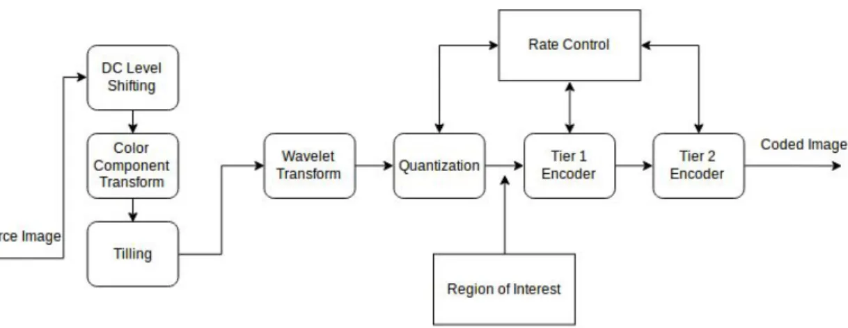
JPEG2000 is an image compression standard, created by the Joint Photographic Experts Group (JPEG) committee in the year 2000, with the intention of superseding their DCT-based image compression standard, JPEG. Based on wavelet decomposition, JPEG2000 is composed of many parts, that deal with a variety of applications. However, for this thesis, only the basic image compression part is relevant. Figure 3.1 contains the block diagram of a JPEG2000 encoder.

Figure 3.1: JPEG2000 encoder block diagram. Some of the main features of JPEG2000 are:

• Superior low bit-rate performance: when compared to the baseline JPEG; • Continuous tone and bi-level image compression;

• Large dynamic range of the pixels: JPEG2000 allows for the (de)compression of images with various dynamic ranges for each color component;

• Lossless and lossy compression: JPEG2000 can provide both the lossless and the lossy mode of image compression;

• Fixed size can be preassigned: The user can select a desired size for the compressed file;

• Region Of Interest (ROI) coding: Sometimes an image contains parts that are of greater importance, with JPEG2000 it is possible to encode parts of an image with higher quality(even lossless) compared to the less important parts;

• Random access and compressed domain processing:with JPEG2000 it is possible to manipulate certain areas (or regions of interest) of the image, for example, replace one object in the image with another.

The JPEG2000 compression system is divided into three main phases, the preprocessing phase, the compression phase and the formation of the bitstream.

3.2.1 preprocessing

The preprocessing phase is composed of three optional operations, DC level shifting,

multi-component transformation and tilling.

DC level shifting

DC level shifting before transformation, and like in the baseline JPEG standard, the pixel values are level-shifted by 2B−1 _{where B is the number of bits per value used for each} component of a pixel. DC level shifting is only applied if the pixel values are unsigned.

Multicomponent transform

Multicomponent transform is the transformation of the image color space into another color space. JPEG2000 supports two multicomponent transformations, a reversible color transform and a irreversible color transform. The reversible color transform transforms the original Red, Green and Blue (RGB) values into YUV values and allows for a lossless reversible transform back to RGB and is done using the following formulas:

       Y =hR+2G+B₄ i U = B − G V = R − G        ,

and the inverse:

       R = V + G G = Y −hU +V₄ i B = U + G        .

The irreversible color transform is the same used in baseline JPEG and introduces error because it uses non integer coefficients on the transformation formulas. The formulas used are:        Y = 0, 299R + 0, 587G + 0, 144B U = −0, 16875R − 0, 33126G + 0, 5B V = 0, 5R − 0, 41869G − 0, 08131B        ,

and the inverse:

       R = Y + 1.402V G = Y − 0.34413U − 0.71414V B = Y + 1.772U        . Tilling

Tilling consists of dividing the image into non overlapping tiles (blocks), all the tiles have the same size, except those at the boundaries when image dimension is not a multiple of the tiles dimension. Tile size is variable up to the size of the original image (unlike baseline JPEG). Each image component is represented at the same tile, i.e., on a gray scale image a tile contains one component, on a multi component image a tile contains all components. For very low bit-rate compression some visible artifacts may appear due to heavy quantization, like in JPEG or any other block transform coding.

Figure 3.2: Example of the blocking artifacts [34].

3.2.2 Compression

After the preprocessing phase comes the compression, which can be divided into three sequential phases, the Discreet Wavelet Transform (DWT), quantization and entropy encoding. Firstly the DWT coefficients are calculated and quantized using a midtread quantizer and then they are coded using the embedded block coding with optimized truncation (EBCOT) [35] algorithm. According to T. Acharya and P.-S. Tsai: "The main drawback of the JPEG2000 standard compared to current JPEG is that the coding algorithm is much more complex and the computational needs are much higher." [8].

3.3

JPEG-LS

JPEG-LS [9] is a standard for lossless and near-lossless compression of continuous tone still images. It has been developed by the Joint Photography Experts Group(JPEG), like JPEG and JPEG2000, with the aim of providing better compression efficiency than lossless JPEG whilst keeping the standard with low complexity. Generally JPEG-LS provides better compression ratios and coding speeds when compared with PNG [36], [37]. When the initial proposals for the new lossless compression standard were requested the following requirements were defined[38]:

1. Provide lossless and near-lossless compression. 2. Target 2 to 16 bit still images.

3. Applicable over wide variety of content.

4. Should not impose any size or depth restrictions.

5. Field of applicability include Medical, Satellite, Archival etc. 6. Implementable with reasonable complexity.

8. Capable of working with a single pass through data.

JPEG-LS is based on the LOw COmplexity LOssless COmpression for Images (LOCO-I) algorithm that, like PNG, relies on prediction however, unlike PNG, uses context modeling of the residuals prior to encoding. Figure 3.3 contains the basic block diagram of JPEG-LS.

Figure 3.3: JPEG-LS block diagram [39].

3.3.1 Prediction

For prediction a fixed predictor is used , the Median Edge Detection (MED) predictor [40], which adapts whenever it finds local edges. This predictor takes into account vertical and horizontal edges, by examining the North, West and Northwest neighbors of the current pixel.

3.3.2 Context modeling

JPEG-LS makes use of a very simple context model where each pixel is assigned to a context. Contexts are determined by three values based on the neighboring pixels of the pixel to be predicted. These gradients represent an estimate of the local gradient, thus capturing the level of activity (smoothness, edginess) allowing JPEG-LS to exploit higher-order structures such as texture patterns and local activity in the image for further compression gains. A more detailed look at context modeling in JPEG-LS is available at [39].

3.3.3 Coding

In JPEG-LS, prediction errors are encoded using a special case of Golomb codes [41] which is also known as Rice coding [42]. These codes are optimal for data that follows a two-sided geometric distribution centered at zero, in which the occurrence of small values is significantly more likely than large values.

On low entropy images or image regions Rice codes are not optimal as the best coding rate achievable is 1 bit per symbol. JPEG-LS uses an alphabet extension mechanism, in order to effectively code this regions, that switches to a run-length mode when a uniform region is encountered.

3.3.4 Near-Lossless Compression

Besides lossless compression, JPEG-LS also provides a lossy mode of operation where the maximum absolute error between the original and reconstructed values can be controlled by the encoder, known as the near-lossless mode. This mode will not be used throughout this thesis.

3.4

H.264

H.264, also known as Advanced Video Coding (AVC), is a video compression standard, created by the Joint Video Team (JVT), consisting of VCEG (Video Coding Experts Group) of ITU-T (International Telecommunication Union—Telecommunication standardization sector), and

MPEG (Moving Picture Experts Group) of ISO/IEC in 2003.

It is a widely used standard that originated from the need for higher compression efficiency, when compared to the older standards, the need for support of special video applications, like DVD storage, video conferencing, video broadcasting and streaming, but also to achieve greater reliability. Figure 3.4a contains a typical encoder block diagram of H.264 while Figure 3.4b contains the typical decoder block diagram of H.264.

(a) Typical H.264 encoder block diagram.

(b) Typical H.264 decoder block diagram. Figure 3.4: H.264 codec block diagrams [11].

several other profiles are also defined. Each profile contains a set of encoding functions, and each is intended for different video applications. The baseline profile is designed for video telephony, video conferencing, and wireless communication. The extended profile is intended for streaming video and audio. The main profile is designed to handle television broadcasting and video storage. The high profile is designed for achieving significant improvement in coding efficiency for higher fidelity material, such as high definition TV/DVD. The main components of each profile can be found at Figure 3.5. A more in depth description of each profile can be found at [11], [12] and for the high profile [13].

Figure 3.5: H264 profile components [13].

In H.264 each picture is divided into a series of Macroblocks (MBs). A MB corresponds to a block of 16x16 pixels which can be subdivided into smaller blocks and partitioned into luma and chroma components to be processed separately. MBs can be considered the basic coding unit in H.264.

To aid in transmission or streaming H.264 provides some high level networking headers and flags. However, the coded video data is stored in units, known as slices. Each slice is divided into the slice header and the slice data, which is a series of coded MBs. There are several types of slices:

• I slices contain intra predicted macroblocks.

• P slices contain intra or inter predicted macroblocks from only one reference.

• B slices contain intra or inter predicted macroblocks from one or two references (biprediction). Type B slices are used in the main profile.

• SP and SI slices are specially-coded slices that enable, among other things,efficient switching between video streams and efficient random access for video decoders. They are used in the extended profile [43].

Figure 3.6: High level overview of a H.264 bitstream hierarchy [44].

3.4.1 Intra-picture prediction

As previously mentioned, intra-picture prediction exploits the spatial correlation among pixels, like image compression.

In H.264 the image is divided into blocks, which will be subtracted by a prediction block P, obtaining the residuals. P is based on the previously encoded block, exploiting the spatial correlation between sequential blocks.

In H.264 intra-picture prediction is divided into three types. The luma 4x4 block, the luma 16x16 macroblock and the chroma prediction. The luma block prediction modes consist of 8 directional modes for edge detection and a mean-based method (DC prediction). The luma macroblocks prediction modes only take into account horizontal or vertical edges, the same mean-based method (DC prediction) available for the luma blocks and a planar method that detects areas of smoothly varying luminance. The chroma components prediction is similar to

the luma macroblock prediction modes. Figure 3.7a contains a graphical representation of the 4x4 luma blocks prediction modes. Figure 3.7b contains a graphical representation of the 16x16 luma blocks and chroma blocks prediction modes.

(a) 4x4 luma block prediction modes.

(b) 16x16 luma block and chroma block prediction modes. Figure 3.7: H.264 intra-picture prediction modes [44].

3.4.2 Inter-picture prediction

Inter-picture prediction, unlike intra-picture prediction, exploits the temporal redundancy in a sequence of frames, the temporal correlation is reduced by the use of motion estimation and compensation algorithms. Using a block-based motion compensation, H.264 creates a prediction model from one or more previously encoded video frames.

The most important differences between inter-picture prediction in H.264 and the older standards is the support for a range of block sizes (from 16x16 to 4x4) and more precise subsample motion vectors (quarter-sample resolution for the luma component). An example of motion estimation with integer and subpixel reference blocks can be found at Figure 3.8.

(a) (b) (c)

Figure 3.8: H.264 inter-picture prediction motion estimation [44]. (a) contains a 4x4 block in the current frame. (b) contains the reference block in the reference frame. (c) contains a subpixel reference block.

3.4.3 Transform and Quantization

H.264 uses different transform methods, depending on the type of residual data to be transformed. For the DC coefficient blocks obtained from the prediction of intra luma macroblocks and from the prediction of chroma DC coefficients a Hadamard transform [45] is used, for everything else a DCT-based transform is used. The output coefficients of the transform are then quantized. Quantization reduces the precision of the transform coefficients according to the quantization parameter (QP).

3.4.4 Deblocking filter

One of the new features that H.264 contains when compared to the older standards is the deblocking filter. The deblocking filter consists of a filter that is applied to each decoded macroblock to reduce blocking artifacts that are introduced after the transform is applied. The deblocking filter is applied after the inverse transform in the encoder and in the decoder. The filter smooths block edges, improving the appearance of decoded frames. The filtered image is the one that is used for motion-compensated prediction of future frames which might improve the compression efficiency, because the filtered image is often a better approximation of the original frame than the blocky image obtained from the inverse transform. Figure 3.9 contains the effect of the deblocking filter on a grayscale image.

(a) Without deblocking filter. (b) With deblocking filter. Figure 3.9: Effect of the deblocking filter [12].

3.4.5 Coding

H.264 uses several coding methods depending on the profile chosen or data that is going to be coded. For the baseline profile, high level headers and flags are encoded using Fixed Length Codes (FLC). For the quantized coefficient values Context-Adaptive Variable Length Coding (CAVLC) is used. For the rest of the data, such as low level flags and parameters, exponential Golomb codes are used. For the main profile, instead of using CAVLC and exponential Golomb codes, H.264 uses Context-Adaptive Binary Arithmetic Coding (CABAC) [46].

3.5

H.265

H.265, also known as High Efficiency Video Coding (HEVC), is a state of the art video compression standard, the successor of the widely used AVC standard (H.264). Like H.264 it is the result of a collaboration between the ITU-T Video Coding Experts Group (VCEG) and the ISO/IEC Moving Picture Experts Group (MPEG). H.265 can be considered an extension of the older H.264 standard, with improvements on the coding efficiency achieved by further exploring existing techniques but with the cost of increasing the complexity of the encoder. Despite having some new design aspects that improve flexibility for operation on several applications and network environments while improving robustness to data losses, the high level syntax architecture used in H.264 has mostly been retained in H.265. Figure 3.10 contains a typical H.265 encoder block diagram.

Figure 3.10: Typical H.265 encoder block diagram [14].

H.265 supports a broad range of applications. This is possible due to some variation in capabilities and functionalities in H.265. This variation is handled by specifying multiple profiles. In many applications, it is currently neither practical nor economical to implement a decoder capable of dealing with all hypothetical uses of the syntax within a particular profile. In order to deal with this problem each profile is subdivided into levels. A level is a specified set of constraints, imposed on values of the syntax elements in the bitstream. These constraints may be simple limits on values, i.e., levels can establish a limit on the picture resolution, frame rate, buffering capacity, and other aspects that are matters of degree rather than basic feature sets. However, this does not solve all problems. Professional environments often require much higher bit rates for better quality than consumer applications, for the same level. This was solved by introducing the concept of tiers, which define the bit rate that the level is able to handle. Several levels in H.265 have both a Main tier and a High tier, based on the bit rates they are capable of handling. H.265 defines several profiles, levels and tiers. For the first version of this standard only three profiles existed, the main profile, the main still picture profile and the main 10 profile. Following the newer releases of H.265, several other profiles were added that extend or improve upon these three profiles.

One of the new changes brought by H.265 is the discontinuation of Macroblocks (MBs) and the introduction of Coding Tree Units (CTUs), which conceptually are similar to MBs but with support for a wider range of sizes (16x16 up to 64x64) and improved sub-partitioning. A CTU represents the basic coding unit in H.265. Each CTU can then be partitioned into smaller blocks, the Coding Units (CUs).

3.5.1 Intra-picture prediction

H.265 has two intra-picture prediction categories, the Angular prediction methods form the first category and provide the encoder with the possibility to model structures with angular edges, the second category is composed of planar prediction and DC prediction that provide the possibility to estimate smooth image structures. The angular prediction methods are similar to the directional modes from H.264 but with support to a wider range of directions (angles). The planar prediction and the DC prediction are the same as the ones used in H.264 with the same name. The total number of intra prediction modes is thirty five, planar taking the first slot, DC the second and angular prediction taking the remaining 33 slots. Figure 3.11 contains a graphical representation of the intra-picture prediction modes of H.265.

Figure 3.11: Intra-picture prediction in H.265 [15].

3.5.2 Inter-picture prediction

Inter-picture prediction in H.265 is an improvement from the older H.264. A significant improvement, besides the greater flexibility in partitioning the blocks, is the ability to encode motion vectors with much greater precision, giving a better predicted block with less residual error. There is also the introduction of a new tool called Advanced Motion Vector

Prediction (AMVP) that improves the predictive coding of the motion vectors. A detailed list of all improvements in inter prediction from the older H.264 can be found at [15]. Figure 3.12 contains a block diagram of HEVC inter-picture prediction module.

Figure 3.12: Inter prediction-picture in H.265 [15] ,blocks in faded gray represent the bi-prediction path.

3.5.3 Transform and Quantization

H.265 specifies two-dimensional transforms of various sizes from 4x4 to 32x32 that are finite precision approximations to the DCT. In addition, H.265 also specifies an alternate 4x4 integer transform based on the Discreet Sine Transform (DST) for use with 4x4 luma Intra prediction residual blocks. The H.265 quantizer design is similar to that of H.264.

3.5.4 Filters Deblocking filter

The deblocking filter in H.265 is similar to the deblocking filter in H.264. However, some changes were made to improve efficiency and support for parallel processing. At the cost of subjective quality, the deblocking filter is only applied to the block boundaries that lie at the luma and chroma sample positions that are multiples of eight. This reduces computational complexity which improves efficiency. It also improves parallel processing by preventing cascading interactions between nearby filtering operations. In H.264 the deblocking filter is applied to vertical or horizontal edges of 4x4 blocks in a MB.

Sample Adaptive Offset filter

One of the new features introduced in H.265 is the Sample Adaptive Offset filter (SAO). The SAO consists of a filter that is designed to remove or reduce the mean sample distortion of a region. It works by first classifying the region samples into multiple categories with a selected classifier, obtaining an offset for each category, and then adding the offset to each sample of the category, where the classifier index and the offsets of the region are coded in the bitstream.

The SAO is applied to the output of the deblocking filter. A more detailed introduction to the Sample Adaptive Offset filter (SAO) is available at [47].

3.5.5 Coding

H.265 uses the same entropy coding method that the main profile of H.264 uses, Context-Adaptive Binary Arithmetic Coding (CABAC) [46] , with a mixture of zero-order exponential golomb codes [44] .

3.5.6 BPG

BPG is a file format for compressed images, based on a subset of the intra-picture mode of H.265. H.265 contains several profiles defined for still-picture coding. These profiles use the intra-frame encoding with various bit depths and color formats. Some of those profiles are the Main Still Picture, Main 4:4:4 Still Picture, and Main 4:4:4 16 Still Picture profiles. BPG is a wrapper for the Main 4:4:4 16 Still Picture Level 8.5 H.265 profile, with only up to 14 bits per sample. BPG uses a slightly different bitstream format that is based on H.265 but strips all the unnecessary headers for image compression. A complete specification can be found here [10].

3.6

Experimental Results

Most of the codecs used throughout this thesis provide extensive customization parameters. The idea of testing all the possibilities is unrealistic, so a subset of the codecs functionality was chosen for these experiments. The subset was the following:

• PNG with compression level of 1, 3, 6 and 9. • JPEG with qualities 80, 90, 95 and 99.

• Theora with quality 10 and 7 (corresponds to qualities 63 and 44 used in the previous chapter).

• JPEG-LS with default settings.

• JPEG2000 with compression ratios of 5x, 10x, 20x and 40x and also lossless mode. • H.264 and H.265 with a Constant Rate Factor (CRF) of 13 and 28, the lossless mode

was also tested, each parameter was tested with two presets, medium and ultrafast. • BPG with a quantizer parameter (similar to CRF) of 13 and 28, the lossless mode was

also tested, each parameter was tested with a compression level of 1 and 5 (fast and medium).

To determine the efficiency of the codecs we execute a script that first compresses and decompresses the dataset sequentially with all the combinations provided in the subset above and lastly calculates the average Peak Signal to Noise Ratio (PSNR) for all the targets.

Figure 3.13: Simplified block diagram of the experiment procedure.

We focus on two important metrics when determining the efficiency of the compression standards, the speed efficiency and the compression efficiency. In order to determine the speed efficiency of a compression standard both the compression and decompression times are measured. All compression and decompression times are obtained with the Linux time utility. The experiment is executed with maximum priority to avoid context switches and other interruptions that would change the fairness of the experiment. The command to execute with maximum priority is presented bellow:

$ sudo chrt -f 99 bash experiment.sh &> result.txt

After the compression and decompression times are recorded, the size (in MiB) is taken into account and the average of bits per pixel (bpp) is calculated for each standard. For obtaining the relation between the number of bits per pixel (bpp) and PSNR a broader subset of codec qualities for each lossy standard was used:

• JPEG with a quality range of 10:100 with a step of 10. • Theora with a quality range of 1:10 with a step of 3.

• JPEG2000 with compression ratios of 5x, 10x, 20x, 40x, 80x and 100x.

• H.264 and H.265 with a CRF range of 1:51 with a step of 5 at the ultrafast preset. • BPG with a CRF range of 1:51 with a step of 5 and compression level 1.

The experimental results are discussed in three parts. The first part considers the results for the lossless codecs, the second part considers the results for the lossy codecs and the third part contains the relation between the number of bits per pixel (bpp) and the average PSNR of the lossy codecs. For this experiment we use three image datasets: The Alboi moving (Appendix B.1) and Alboi mixed (Appendix B.2) image datasets and the P0 Large image

dataset (Appendix B.4).

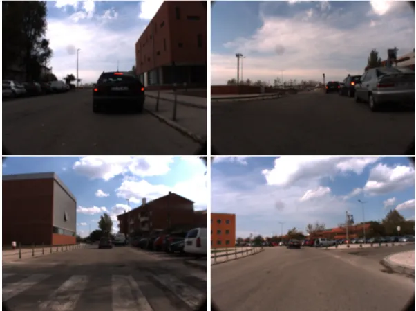
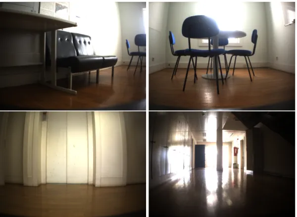
Both the Alboi moving and Alboi mixed image datasets contain image sequences from the Alboi bag (Appendix A.1, Figure 3.14) with a resolution of 1624x1224 pixels. The P0 Large image dataset contains images from the P0 Large bag (Appendix A.2, Figure 3.15) with a resolution of 1296x964 pixels. The Alboi moving image dataset contains image sequences with movement. The Alboi mixed image dataset contains mixed image sequences, the first half consists of still image sequences and the second half of motion image sequences. The P0 Large image dataset contains still image sequences.

Figure 3.14: Example frames from the Alboi bag.

3.6.1 Lossless

Table 3.1 presents the speed efficiency results for the lossless modes of the compression standards. According to the experimental results presented in Table 3.1 the fastest standard is H.264, followed by PNG with low compression levels and H.265 ultrafast preset. Moreover, JPEG2000, H.265 medium preset mode, JPEG-LS, BPG with low compression level and PNG with medium compression levels provide mediocre speeds while BPG with medium compression levels and PNG with high compression levels provide poor speeds.

In Chapter 3.3 it is mentioned that generally JPEG-LS provides much faster compression speeds than PNG, while this is true for higher compression levels, our experiments show that, with the codec that we used to represent JPEG-LS, PNG with low compression levels is much faster that JPEG-LS.

Alboi moving Alboi mixed P0 Large

C Time(s) D Time(s) C Time(s) D Time(s) C Time(s) D Time(s)

H.264 uf 8 15 8 14 5 9 H.264 md 73 22 70 20 42 11 PNG 1 85 35 97 33 50 22 H.265 uf 127 41 106 39 51 20 PNG 3 115 34 141 33 64 22 JPEG2000 223 161 204 147 135 94 H.265 md 262 35 252 37 125 17 JPEG-LS 329 315 304 290 178 173 PNG 6 364 35 324 33 183 22 BPG fast 388 104 373 97 223 59 BPG md 506 102 493 97 296 59 PNG 9 1087 34 1824 32 732 21

Table 3.1: Speed efficiency of the lossless codecs.

Table 3.2 shows the results for the compression efficiency of the lossless standards in size(MiB) and bits per pixel(bpp). Analyzing the results presented in Table 3.2 it is possible to conclude that BPG is the most compression efficient, followed by JPEG-LS and H.264 medium preset. The worst results belong to PNG, that, when compared to the most efficient standard tested, has more than double bits per pixel. JPEG2000 provides mediocre results in all situations. As expected, both H.264 and H.265 show improvement when we transition to datasets with little to no movement, due to the temporal prediction, which none of the image compression standards use.

Alboi moving Alboi mixed P0 Large Size(MiB) bpp Size(MiB) bpp Size(MiB) bpp

BPG md 292,63 4,12 256,44 3,61 156,87 3,51 BPG fast 292,91 4,12 256,72 3,61 156,99 3,51 JPEG-LS 424,32 5,97 373,52 5,25 229,57 5,14 H.264 md 437,44 6,15 373,56 5,25 218,31 4,89 H.265 md 515,05 7,25 420,95 5,92 239,46 5,36 H.265 uf 550,40 7,74 440,59 6,20 246,70 5,52 H.264 uf 533,20 7,50 462,46 6,51 273,25 6,12 JPEG2000 551,32 7,76 495,71 6,98 307,68 6,89 PNG 9 597,41 8,40 528,07 7,43 325,34 7,28 PNG 6 606,68 8,53 546,57 7,69 332,23 7,44 PNG 3 673,02 9,47 606,73 8,53 371,90 8,32 PNG 1 708,91 9,97 644,27 9,06 391,38 8,76

Table 3.2: Compression efficiency of the lossless codecs.

3.6.2 Lossy

Table 3.3 presents the speed efficiency results for the lossy modes of the codecs used to represent the compression standards. According to the experimental results presented in Table 3.3, and when comparing similar quality levels, the fastest lossy standard is H.264, followed by JPEG and H.265. Theora shows little speed difference when changing quality levels. Both BPG and JPEG2000 are slow. Looking at decompression times, all standards provide similar results with the exception of BPG and JPEG2000 which require substantially more time to decompress.

Table 3.4 shows the results for the compression efficiency of the lossy standards in size (MiB) and bits per pixel (bpp). From the table we can observe, comparing similar qualities, that video compression standards, for the most part, provide the best compression when compared to image compression standards. Moreover, the efficiency of the video compression standards increases whenever movement in the image datasets reduces. Of all the video compression standards H.265 provides the best results followed by H.264 and lastly Theora. When the dataset contains high motion, the image compression standards provide very competitive results. BPG and JPEG2000 provide the best results of all the image compression standards, with BPG providing slightly better results than JPEG2000.

Alboi moving Alboi mixed P0 Large C Time(s) D Time(s) C Time(s) D Time(s) C Time(s) D Time(s)

H.264 28 uf 5 11 4 10 2 7 H.264 13 uf 6 13 6 12 4 7 JPEG 80 15 19 13 19 10 11 JPEG 50 15 19 16 16 10 16 H.265 28 uf 28 12 17 12 6 7 JPEG 90 21 21 19 20 13 12 JPEG 95 25 22 22 22 16 13 H.264 28 md 38 12 23 11 8 7 H.265 13 uf 48 13 33 16 12 8 JPEG 99 37 27 33 26 22 15 Theora 7 62 11 53 10 31 7 H.265 28 md 83 12 55 14 21 7 Theora 10 65 11 56 11 33 7 H.264 13 md 85 14 73 13 37 8 H.265 13 md 148 15 123 19 58 9 BPG 28 fast 177 41 168 38 109 23 BPG 28 md 210 44 199 51 133 28 JPEG2000 40x 230 55 212 48 144 31 JPEG2000 20x 234 59 218 57 147 39 JPEG2000 10x 242 76 223 76 150 51 JPEG2000 5x 253 113 239 111 157 75 BPG 13 fast 300 75 271 68 174 41 BPG 13 md 381 75 339 72 220 45