63
DOMINANCE AT THE DIVISIONAL EFFICIENCIES LEVEL IN NETWORK
DEA: THE CASE OF TWO-STAGE PROCESSES
1Dimitris Sotiros
Universidade Católica Portuguesa, Católica Porto Business School and CEGE, Rua de Diogo Botelho 1327, 4169-005, Porto, Portugal
Gregory Koronakos
Department of Informatics, University of Piraeus, 80, Karaoli and Dimitriou, 18534 Piraeus, Greece
Dimitris K. Despotis
Department of Informatics, University of Piraeus, 80, Karaoli and Dimitriou, 18534 Piraeus, Greece
ABSTRACT
We introduce in this paper the notion of dominance in the divisional efficiencies space in Network Data Envelopment Analysis. We argue that, irrespectively of the method used, a successful efficiency evaluation protocol should satisfy the dominance property at the divisional efficiencies level. In particular, there should not exist any other feasible solution in the assessment model, suboptimal in terms of the optimality criterion, that provides stage efficiencies scores at least as high as the assessed ones and higher for at least one stage. Then, we investigate the dominance property for the relational model and the additive efficiency decomposition method for general two-stage series processes. We provide an example showing that these methods do not comply with the dominance requirement at the divisional efficiencies level and lead to controversial results.
Keywords: Data Envelopment Analysis; network DEA; relational model; efficiency decomposition; dominance
property.
INTRODUCTION
Network DEA is an extension of the conventional DEA, which considers the DMU as a network of sub-DMUs (divisions, sub-units, sub-processes, stages, etc.) and was introduced by Fare and Grosskopf (2000). Thereafter, a large volume of studies has been published in both theoretical and application level. Extended literature reviews can be found in Castelli et al. (2010), Cook and Zhu (2014) and Kao (2014a). In network DEA, the efficiency is a multi-dimensional (vector) measure, as one has to account for the efficiency of the divisions encountered in the process as well as the overall system efficiency. Assessing the efficiency of the individual divisions and the overall efficiency of the system independently of each other constitutes the so called independent efficiency assessments approach (see, for example, Wang et al., 1997 and Seiford and Zhu, 1999). The holistic approach, on the other hand, requires that the efficiencies of the individual divisions and the overall system efficiency are estimated jointly by taking into account the interdependencies of the divisions by means of the flow of intermediate measures. Irrespectively of the method used to assess the efficiencies in the frame of the holistic approach, the divisional efficiencies cannot exceed their independent counterparts, which serve as upper bounds. The series and the parallel
1 Sotiros, D., G. Koronakos and D. K. Despotis (2018) Dominance at the divisional efficiencies level in network
DEA: The case of two-stage processes, in Emrouznejad and Thanassoulis (eds.), Data Envelopment Analysis and Performance Measurement: Recent Developments: Proceedings of the DEA40: International Conference of Data Envelopment Analysis, Aston Business School, UK, ISBN: 978 1 85449 438 2.
64
production processes are two characteristic process configurations studied extensively in the literature. The term “stage” is commonly used to name the divisions in series processes and it will be used equivalently hereafter.
Generally, there are two main paradigms in the holistic approach of network DEA for series processes, namely the non-cooperative and the cooperative. In both paradigms, the efficiency of each division is commonly defined as the ratio of the implied aggregate value of its outputs to the implied aggregate value of its inputs. Focusing on two-stage processes, the non-cooperative paradigm assumes that pre-emptive priority is given to one of the two stages (leader stage), whose efficiency is assessed first. Then, the efficiency of the other stage (follower) is assessed in a manner that the optimal efficiency of the leader is maintained (Liang et al., 2008). In the cooperative paradigm, two broad approaches can be identified, namely the top-down approach and the bottom-up approach. This classification reflects how the different methods select the driver of the assessment, i.e. whether the system (top-down) or the divisional efficiencies (bottom-up) is given priority for optimization. In the top-down approach, the overall system efficiency is optimized first, and the divisional efficiencies derive as offspring from the optimal solution that maximizes the system efficiency. This requires an a priori definition of the overall system efficiency. Representative methods of the top-down approach are the additive efficiency decomposition method (Chen et al., 2009) and the relational model (Kao and Hwang, 2008; Kao, 2009; Kao, 2014b). The latter, when applied to simple two-stage processes where nothing but the external inputs to the first stage enters the system and nothing but the external outputs of the second stage leaves the system, is also known as multiplicative efficiency decomposition method (Kao and Hwang, 2008). The bottom-up approach is based on an inverse perspective. The divisional efficiencies are estimated first and the system overall efficiency is derived ex post. The methods proposed in the literature differ in the way they assess the divisional efficiencies and the functional form used to define the system efficiency. Indicative methods of the bottom-up approach can be found in Guo et al. (2017), Ang and Chen (2016), Despotis et al., (2016a; 2016b; 2016c) and Li et al. (2012). In the methods introduced by Despotis et al. (2016a), (2016b) for series processes, the stage efficiencies are treated as distinct objective functions, and vector-optimization (multi-objective programming-MOP) techniques are used to locate the stage efficiencies as close as possible to their independent counterparts, i.e. the ideal point in terms of MOP terminology. Thus, the notion of Pareto optimality is introduced in the divisional efficiencies space. That given, we argue that the point defined by the individual stage efficiencies scores, irrespectively of the method used to assess them, should lie on the Pareto front in the divisional efficiencies space. As the stage efficiencies are determinant of the system’s overall efficiency, the higher the stage efficiencies are, the higher the overall efficiency of the evaluated DMU is expected to be. Consequently, the stage efficiencies should be non-dominated, whatever the optimality criterion of the assessment model is. Otherwise, we would face the paradox that there are higher stage efficiency scores associated with a lower than the optimal system efficiency. Thus, we argue that, whatever is the approach followed, top-down or bottom-up, the assessment model should comply with the dominance property in the divisional efficiencies space.
In this paper, we investigate the dominance property of the stage efficiency scores in the relational model and the additive efficiency decomposition method for general two-stage series processes. We provide an illustrative counter example that reveals the violation of the dominance property, i.e. there are feasible stage
65
efficiencies that dominate the stage efficiencies estimated by these models, at a lower overall system efficiency. In these cases, we show that the violation of the dominance property leads to controversial results and irregularities.
The paper unfolds as follows. In the next section we introduce the dominance property in the divisional efficiencies space. Then, we investigate the dominance property in the relational model and in the additive efficiency decomposition method. The paper ends with our main conclusions.
THE DOMINANCE PROPERTY IN THE DIVISIONAL EFFICIENCIES SPACE
In this section we introduce the dominance property at the divisional efficiencies level in network DEA and we argue that a successful efficiency assessment should satisfy this property. For this, let us start with the independent assessments approach, where the connections among the divisions are neglected and the divisional and the system efficiencies are assessed independently with standard DEA models. This approach has been criticized because it often leads to controversial results. There are examples where the system may be rendered efficient even though some of the divisions are inefficient (Wang et al., 1997; Kao & Hwang, 2008; Kao, 2014b). Moreover, there are cases where all the divisions of a DMU A are less efficient than the corresponding divisions of another DMU B, but A appears with a higher overall efficiency score than B (Kao &Hwang, 2010).
Treating these irregularities was the core motive for developing the network DEA models that take into account the internal structure of the system and the flow of intermediate measures among its divisions. So, a successful assessment in the frame of network DEA should secure that DMUs with higher divisional efficiencies should show higher overall system efficiency. Consequently, increasing the divisional efficiencies in a system should lead to higher overall system efficiency. Related to this is the Kao’s (2014b) comment: “The processes responsible for most of the inefficiency in a system are identified from the efficiency decomposition. Improving the efficiency of these processes will thus be the most effective way to improve the performance of the system”. At the edge of this property lies the fundamental property, that a DMU is efficient if and only if all its divisions are efficient. To illustrate the above, consider a DMU with two divisions, and A and B two different feasible states of efficiency that the DMU can come to:
State A: [𝑒𝑜(𝐴), 𝑒1(𝐴), 𝑒2(𝐴)]
State B: [𝑒𝑜(𝐵), 𝑒1(𝐵), 𝑒2(𝐵)]
where 𝑒𝑜(. ), 𝑒1(. ) and 𝑒2(. ) denote respectively the system overall efficiency and the divisional
efficiencies. The dominance property at the divisional efficiencies level is stated as follows: 𝑒1(𝐴) > 𝑒1(𝐵) 𝑎𝑛𝑑 𝑒2(𝐴) ≥ 𝑒2(𝐵)
𝑜𝑟
𝑒1(𝐴) ≥ 𝑒1(𝐵) 𝑎𝑛𝑑 𝑒2(𝐴) > 𝑒2(𝐵) } ⟹ 𝑒
𝑜(𝐴) > 𝑒𝑜(𝐵)
This means that if the state of efficiency A dominates the state B at the divisional efficiency level, then the overall system efficiency in state A is greater than that in state B. This property is not method-depended and in that sense, it is universal. If the optimal state of divisional efficiencies assessed by the network DEA model define a non-dominated point on the Pareto front in the divisional efficiencies space, the dominance
66
property is satisfied. Otherwise, the above fundamental property is violated. Notice that the above property is expressed in terms of different states of efficiency of the same DMU (intra-DMU dominance). However, the dominance property should also hold across the optimal states of efficiency of different DMUs (inter-DMU dominance). For instance, if the divisional efficiency scores of (inter-DMU A dominate the divisional efficiency scores of DMU B, then the overall efficiency of DMU A should be higher than the overall efficiency of DMU B. That is, a successful efficiency assessment should secure that the dominance property is satisfied at both the intra-DMU and the inter-DMU levels.
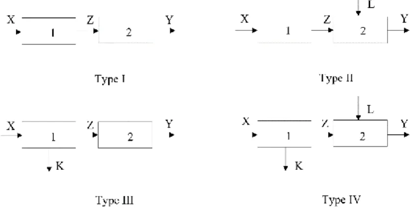
In the following sections, we will show that there are network DEA methods of the top-down approach that do not satisfy the aforementioned dominance property, bringing in the spotlight anomalies observed and criticized in the independent assessments approach. Particularly, we will show that when an optimal state of efficiency is achieved at the system level and the divisional efficiencies derive as offspring of that state, there might be other feasible state of efficiency dominating the optimal one at the divisional efficiencies space at a lower (suboptimal) system efficiency. We will present our observations for the general Type IV two-stage series structure shown in Fig. 1 (c.f. Despotis et al., 2016c).
Figure 1: Two-stage series processes of varying complexity
THE RELATIONAL MODEL
We start our investigation with the general two-stage series structure (Type IV) as presented in Figure 1. The stage efficiencies as well as the overall system efficiency are defined as follows:
0 0 0 0 1 j j j j wZ K e vX + =
,
0 0 0 0 2 j j j j uY e wZ L = +,
0 0 0 0 0 0 j j j j j uY K e vX L + = +Kao (2014b) proposed the following linear program for the efficiency assessment of DMUs with the Type IV structure.
67 0 0 0 0 max . . 1 0, 1, 2,..., 0, 1, 2,..., , , , , j j j j j j j j j j uY K s t vX L wZ K vX j n uY wZ L j n v w u + + = + − = − − = (1)
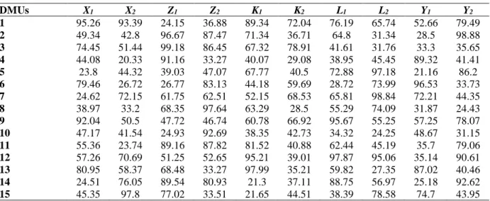
We provide an example below, which shows that model (1) fails to locate the efficiencies of the real processes (divisions-stages) on the Pareto front in the (e1, e2) space. This can be validated by applying the model (1) on the synthetic data presented in Table 1 where the role of the measures X=(X1, X2), Z=(Z1, Z2), K=(K1, K2), L=(L1, L2) and Y=(Y1, Y2) is as depicted in the Type IV structure of Fig. 1.
Table 1: Synthetic data set for the Type IV structure
DMUs X1 X2 Z1 Z2 K1 K2 L1 L2 Y1 Y2 1 95.26 93.39 24.15 36.88 89.34 72.04 76.19 65.74 52.66 79.49 2 49.34 42.8 96.67 87.47 71.34 36.71 64.8 31.34 28.5 98.88 3 74.45 51.44 99.18 86.45 67.32 78.91 41.61 31.76 33.3 35.65 4 44.08 20.33 91.16 33.27 40.07 29.08 38.95 45.45 89.32 41.41 5 23.8 44.32 39.03 47.07 67.77 40.5 72.88 97.18 21.16 86.2 6 79.46 26.72 26.77 83.13 44.18 59.69 28.72 73.99 96.53 33.73 7 24.62 72.15 61.75 62.51 52.15 68.53 65.81 98.84 72.21 44.35 8 38.97 33.2 68.35 97.64 63.29 28.5 55.29 74.09 31.87 24.43 9 92.04 50.5 47.72 46.74 60.78 66.92 95.67 55.25 57.25 78.07 10 47.17 41.54 24.93 92.69 38.35 42.73 34.32 24.25 48.67 31.15 11 55.36 23.74 89.16 87.82 81.52 40.88 62.44 45.19 35.7 79.06 12 57.26 70.69 51.25 52.65 95.21 39.01 97.87 95.06 35.14 90.61 13 80.95 58.37 68.48 33.27 97.99 35.21 59.82 27.35 87.02 40.46 14 24.51 76.05 89.54 80.93 21.3 37.11 88.75 56.97 25.18 92.62 15 45.35 97.8 77.02 33.51 21.65 44.51 38.39 78.58 74.7 43.95
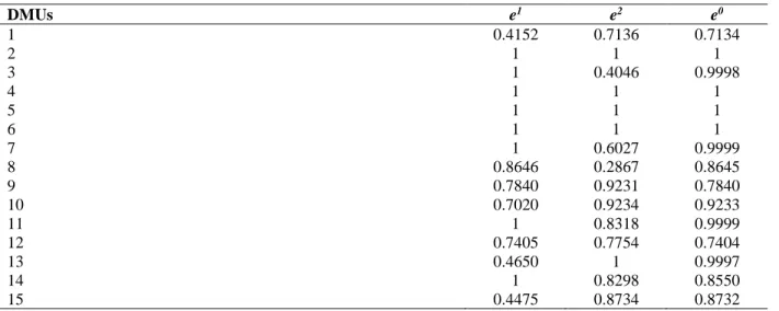
In Table 2, the columns 2-3 present the real efficiency scores of the first and the second stage respectively whereas the column 4 indicates the overall efficiency of the system. For the DMU 8, the real stage efficiencies and the overall system efficiency are respectively e81=0.8646, e82=0.2867 and e =80 0.8645. However, there is a feasible solution in model (7), which provides higher divisional efficiency scores at a lower overall system efficiency (e = , ˆ18 1
2 8
ˆ 0.3401
e = ,e =ˆ80 0.5263). The same anomaly is observed in the DMUs 1, 3 and 13 as presented in Table 3. There are feasible (achievable) divisional efficiencies in model (1) that provide a lower system efficiency, despite they dominate those obtained by model (7). Thus, when the relational model is applied to two-stage processes of the general Type IV, it does not satisfy the dominance property. We also notice that DMU 3 achieves higher overall efficiency than DMU 14, even though the latter achieves higher stage efficiency scores. This peculiarity has been spotted and criticized by Kao and Hwang (2010) for the independent assessment approach.
68 Table 2: Results obtained from model (1)
DMUs e1 e2 e0 1 0.4152 0.7136 0.7134 2 1 1 1 3 1 0.4046 0.9998 4 1 1 1 5 1 1 1 6 1 1 1 7 1 0.6027 0.9999 8 0.8646 0.2867 0.8645 9 0.7840 0.9231 0.7840 10 0.7020 0.9234 0.9233 11 1 0.8318 0.9999 12 0.7405 0.7754 0.7404 13 0.4650 1 0.9997 14 1 0.8298 0.8550 15 0.4475 0.8734 0.8732
The same anomalies are observed when the relational model is applied in two-stage processes of Types II and III. Specifically, the point defined by the individual stage efficiencies scores, by the relational method does not lie on the Pareto front in the divisional efficiencies space. Additionally, it can be observed that a DMU with higher divisional efficiencies scores than another one, may quaintly achieve a lower overall efficiency score than the second one. To this end, in general, the relational does not comly with the dominance property. However, in the elementary Type I structure, the relational model does comply both with the inter-DMU and inter-DMU dominance property.
Table 3: Dominating stage efficiencies that are feasible in model (1)
DMUs 𝒆̂𝟏 𝒆̂𝟐 𝒆̂𝟎
1 0.6255 1 0.6255
3 1 0.6522 0.6530
8 1 0.3401 0.5263
13 0.6905 1 0.6905
THE ADDITIVE EFFICIENCY DECOMPOSITION METHOD
Chen et al. (2009) introduced the additive efficiency decomposition method for the elementary two-stage process of Type I, which, however, is straightforwardly extendable to the other Types II-IV. The overall efficiency of the evaluated DMU j0 (system) is defined as a weighted average of the stage efficiencies, i.e.
0 0 0 0 0 0 1 1 2 2 j j j j j e =t e +t e with 0 0 1 2 1 j j
t +t = , where the weights
(
)
0 0
1 2
,
j j
t t are defined endogenously as functions of the decision variables. Regarding the Type IV structure, the stage efficiencies as well as the overall one are
0 0 0 0 1 j j j j wZ K e vX + = , 0 0 0 0 2 j j j j uY e wZ L = + , 0 0 0 0 0 0 0 0 0 0 0 0 1 1 2 2 j j j j j j j j j j j wZ uY K e t e t e vX wZ L + + = + =
+ + and can be derived by the linear model (2).
69 0 0 0 0 0 0 max . . 1 0, 1, 2,..., 0, 1, 2,..., , , , , j j j j j j j j j j j j wZ uY K s t vX wZ L wZ K vX j n uY wZ L j n v w u + + + + = + − = − − = (2)
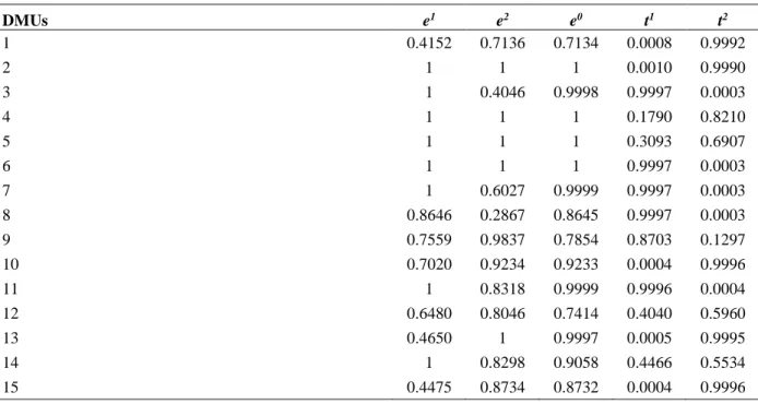
We use the fifteen synthetic DMUs depicted in Table 1 to show that model (2) does not provide stage efficiencies scores on the Pareto front in the divisional efficiencies space. Table 4 exhibits the results obtained by model (2) for the data depicted in Table 1, i.e. the stage efficiencies (columns 2-3), the overall efficiency (column 4) and the weights assigned to the two stages (columns 5-6). In this example, we observe the aforementioned anomaly in four DMUs, namely the DMUs 1, 3, 8 and 13. The Table 5 depicts dominating stage efficiencies for these DMUs, which are feasible in model (2), as well as their overall efficiency and the weights assigned to the stage efficiencies. Notice that the stage efficiency scores presented in Table 5 coincide with the independent efficiency scores of the two stages for each DMU and the Pareto front degenerates to the ideal point in the two-dimensional space( ,e e1 2).
Table 4: Results obtained from model (2)
DMUs e1 e2 e0 t1 t2 1 0.4152 0.7136 0.7134 0.0008 0.9992 2 1 1 1 0.0010 0.9990 3 1 0.4046 0.9998 0.9997 0.0003 4 1 1 1 0.1790 0.8210 5 1 1 1 0.3093 0.6907 6 1 1 1 0.9997 0.0003 7 1 0.6027 0.9999 0.9997 0.0003 8 0.8646 0.2867 0.8645 0.9997 0.0003 9 0.7559 0.9837 0.7854 0.8703 0.1297 10 0.7020 0.9234 0.9233 0.0004 0.9996 11 1 0.8318 0.9999 0.9996 0.0004 12 0.6480 0.8046 0.7414 0.4040 0.5960 13 0.4650 1 0.9997 0.0005 0.9995 14 1 0.8298 0.9058 0.4466 0.5534 15 0.4475 0.8734 0.8732 0.0004 0.9996
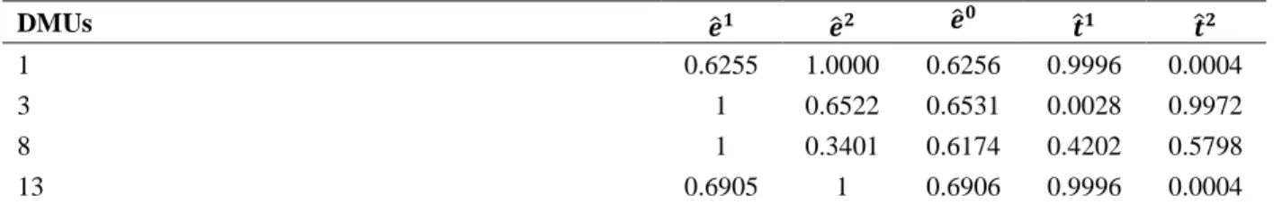
The figures in Table 5 reveal the paradox that higher stage efficiencies provide lower system efficiency. Thus, the additive decomposition method does not comply with the dominance property when is applied in two-stage processes of type IV. As a result, comparisons among DMUs may also lead to unjustifiable
70
results. For instance, DMU 9 has higher performance in both stages than DMU 10, but the latter one achieves a higher overall efficiency score (see Table 4).
Table 5: Feasible dominating stage efficiencies in model (2)
DMUs 𝒆̂𝟏 𝒆̂𝟐 𝒆̂𝟎 𝒕̂𝟏 𝒕̂𝟐
1 0.6255 1.0000 0.6256 0.9996 0.0004
3 1 0.6522 0.6531 0.0028 0.9972
8 1 0.3401 0.6174 0.4202 0.5798
13 0.6905 1 0.6906 0.9996 0.0004
The results of the additive efficiency decomposition method when applied to Type II-III structures have the same peculiarities. However, this method complies with the dominance property when it is applied to the elementary Type I structure.
CONCLUSIONS
We revisited in this paper some characteristic NDEA methods, whose formulation is originally based on the multiplier form of the DEA models, to investigate whether they possess the dominance property at the divisional efficiencies level. It is of no doubt that the divisional efficiencies in a multi-division system are determinants of the overall system efficiency. Thus, the higher are the efficiencies of the divisions the higher is the system efficiency. Based on this basic principle, we introduced the dominance property as a minimal requirement that the NDEA methods should satisfy, regardless the optimality criterion used to assess the overall and the divisional efficiencies of a system. The dominance property should be satisfied at two levels; the intra-DMU and inter-DMU level. The intra-DMU dominance property secures that there should not exist any other feasible solution in the assessment model, suboptimal in terms of the optimality criterion, that provides stage efficiencies scores at least as high as the assessed ones and higher for at least one stage. Analogously, the inter-DMU dominance property ensures that across DMU comparisons the higher the divisional efficiency scores are, the higher is the system efficiency.
We restrained our investigation to two-stage processes of varying complexity and two representative methods that follow the top-down approach, namely, the relational model and the additive efficiency decomposition approach. We provided a counter example to show that the additive efficiency decomposition method and the relational model do not satisfy the dominance property when they are applied to Type IV two-stage processes. The dominance property is also violated when these two methods are applied to Type II-III structures. However, regarding the elementary Type I structure, both methods comply with the dominance property (see also Koronakos et al. 2018). The modification of the additive efficiency decomposition method and the relational model so as to comply with the dominance property in general structures are issues for future research.
Representative methods that follow the bottom-up approach are the leader-follower method (Liang et al., 2008), the Multiplicative aggregation method (Li et al., 2012), the Additive aggregation method (Ang and Chen, 2016; Guo et al., 2017) the min-max method (Despotis et al., 2016c) and the weak-link method
71
(Despotis et al., 2016b). These methods resort to multi-objective programming techniques to locate a point on the Pareto front in the divisional efficiency space. Thus, they comply with the dominance property at the intra-DMU level. Moreover, deriving the overall efficiency in these methods by an increasing function of the divisional efficiencies, the dominance property is satisfied at the inter-DMU level as well. Consequently, the methods that follow the bottom-up approach comply with the dominance property.
ACKNOWLEDGEMENTS
This work has been partly supported by the University of Piraeus Research Center.
REFERENCES
[1] Ang, A., & Chen C.M. (2016). Pitfalls of decomposition weights in the additive multi-stage DEA model. Omega, 58, 139-153.
[2] Castelli, L. Pesenti, R., & Ukovich, W. (2010). A classification of DEA models when the internal structure of the Decision-Making Units is considered. Annals of Operations Research, 173(1), 207-235.
[3] Chen, Y., Cook, W.D., Li, N., & Zhu, J. (2009). Additive efficiency decomposition in two-stage DEA. European
Journal of Operational Research, 196(3), 1170-1176.
[4] Cook, W.D., & Zhu, J. (2014). Data Envelopment Analysis - A Handbook of Modeling Internal Structure and
Network. New York: Springer.
[5] Despotis, D.K., Koronakos, G., & Sotiros, D. (2016a). Composition versus decomposition in two-stage network DEA: A reverse approach. Journal of Productivity Analysis, 45(1), 71-87.
[6] Despotis, D.K., Koronakos, G., & Sotiros, D. (2016b). The “weak-link” approach to network DEA for two-stage processes. European Journal of Operational Research, 254(2), 481-492.
[7] Despotis, D.K., Sotiros, D., & Koronakos, G. (2016c). A network DEA approach for series multi-stage processes.
Omega, 61, 35-48.
[8] Fare R, Grosskopf S (2000). Network DEA. Socio-Economic Planning Sciences, 34(1), 35-49.
[9] Guo, C., Shureshjani, R.A., Foroughi, A.A., & Zhu, J. (2017). Decomposition weights and overall efficiency in two-stage additive network DEA. European Journal of Operational Research, 257(3), 896-906.
[10] Kao, C. (2009). Efficiency measurement for parallel production systems. European Journal of Operational
Research, 196(3), 1107–1112.
[11] Kao, C. (2014a). Network data envelopment analysis: A review. European Journal of Operational Research, 239(1), 1–16.
[12] Kao, C. (2014b). Efficiency decomposition for general multi-stage systems in data envelopment analysis.
European Journal of Operational Research, 232(1), 117-124.
[13] Kao, C., & Hwang, S.N. (2008). Efficiency decomposition in two-stage data envelopment analysis: An application to non-life insurance companies in Taiwan. European Journal of Operational Research, 185(1), 418– 429.
[14] Kao, C., & Hwang, S. N. (2010). Efficiency measurement for network systems: IT impact on firm performance.
Decision Support Systems, 48(3), 437–446.
[15] Koronakos, G., Sotiros, D., & Despotis, D.K. (2018). Reformulation of Network Data Envelopment Analysis models using a common modelling framework. European Journal of Operational Research, https://doi.org/10.1016/j.ejor.2018.04.004.
[16] Li, Y., Chen, Y., Liang, L., & Xie, J. (2012). DEA models for extended two-stage network structures. Omega, 40(5), 611-618.
72
[17] Liang, L., Cook, W.D., & Zhu, J. (2008). DEA models for two-stage processes: Game approach and efficiency decomposition. Naval Research Logistics, 55(7), 643-653.
[18] Seiford, L.M., & Zhu, J. (1999). Profitability and Marketability of the Top 55 U.S. Commercial Banks.
Management Science, 49(9), 1270-1288.
[19] Wang, C.H., Gopal, R.D., & Zionts, S. (1997). Use of Data Envelopment Analysis in assessing Information Technology impact on firm performance. Annals of Operations Research, 73, 191-213.