M
ESTRADO EM
E
CONOMETRIA
A
PLICADA E
P
REVISÃO
T
RABALHO
F
INAL DE
M
ESTRADO
D
ISSERTAÇÃO
A
N
O
RDERED
P
ROBIT
A
NALYSIS OF
S
OCIAL
M
OBILITY IN
P
ORTUGAL
M
ARIA
T
ERESA
L
OUSADA DE
F
REITAS
M
ONTEIRO
O
RIENTAÇÃO
:
P
IERRE
H
OONHOUT
An Ordered Probit Analysis of Social Mobility in Portugal
Teresa Freitas Monteiro
November 27, 2017
Abstract
Contents
1 Introduction 4
2 Social and Income Mobility: A short review 5
2.1 Mobility concepts . . . 5
2.2 Economic approach to social mobility . . . 6
2.2.1 Mobility’s multiple dimensions . . . 6
2.2.2 Mobility Measures . . . 8
2.2.3 Definition of thresholds . . . 8
2.3 Ordered probit and mobility . . . 10
3 Econometric Theory 11 3.1 Ordered Probit . . . 11
3.1.1 Estimation by Maximum Likelihood . . . 12
3.1.2 Predicted Probabilities and Marginal Effects . . . 13
3.2 Comparison of Predicted Probabilities . . . 13
4 Data Treatment and Analysis 15 4.0.1 Cleaning the data and Sampling . . . 16
4.1 Defining income classes . . . 17
4.2 Descriptive statistics . . . 17
5 Estimation and Results 19 5.1 Ordered probit applications to income mobility, conditional on past status . . . 19
5.2 Average Predicted Probabilities . . . 20
5.3 Average Marginal Effects . . . 20
5.4 A short note on the generalized ordered probit . . . 22
6 Conclusion 23 A Appendices 31 A.1 Data treatment and analysis . . . 31
A.1.1 Tax Band Notes . . . 31
A.1.2 Statistics . . . 31
A.2 Estimation Results Tables . . . 35
A.2.2 Predicted Probabilities . . . 39
A.2.3 Marginal Effects . . . 44
A.3 Generalized Ordered Probit . . . 54
A.3.1 Parallel Regression Assumption . . . 54
1
Introduction
This study proposes the use of an ordered probit model to analyse income mobility in the private sector in Portugal using Quadros do Pessoal dataset, an annual census survey conducted by the Portuguese Ministry of Solidarity and Social Security (MSSS). The first objective is to answer the question ”what is the probability of an individual to come up/down in the income ladder” (across income classes and time). The second objective is to look at ”how individual characteristics affect these probabilities”. The approach used in this study provides a methodology to evaluate income class mobility and to quantify how certain characteristics or events impact the probability of moving up across the different social classes.
The first comprehensive treatment of ordered regression model (ORM) appeared in a study by McK-elvey and Zavoina (1975) where they analyse the votes (against, weakly for or string) for the 1965 US Medicare bill. In its essence, an ordered regression model maps a naturally ordered preference scale (usu-ally unobserved) to an ordered observed outcome. This study uses an ordered probit (oprobit) model which derives from the ORM when choosing a normally distributed random term1. The ordered regres-sion models have been used in a variety of studies, some applications include: Winship and Mare (1984) use an oprobit to model educational attainment; Terza (1985) applies it to bond ratings; Clark et al. (2001), and Wim and Ven den Brink (2002) use it to explain levels of ”life satisfaction”; Long and Freese (2006) take on an ologit to evaluate responses to the question ”A working mother can establish just as warm and secure a relationship with her child as a mother who does not work”; Riphahn et al. (2005) also use an ologit to analyse individual data on health care satisfaction; among others. After McKelvey and Zavoina (1975), generalizations of the ordered response models have been proposed such as the generalized thresholds model (Maddala, 1983; Terza, 1985) and the sequential model (Fienberg, 1980; Tutz, 1990)
In this study the categorical dependent variable in the ordered probit model is ”Income Class”. This variable is created by dividing private sector workers into 4 income classes (low, middle-low, middle-high and high) where the division is made according to which IRS average tax band the worker’s nominal wage would fall into. Worker’s characteristics such as gender, age group, highest educational attainment and tenure are included as explanatory variables. Further, worker’s data is taken at two different waves, the first wave constituted by the same workers observed at 2000 and 2003 and the second wave constituted by the same workers observed at 2006 and 2009. An ordered probit model per income class of the form P(yt = j | x, yt 1 = s), is run separately for each wave, where j, s = 0,1,2,3 represent the income
categories.
To measure mobility, we test formally if the predicted probabilities from the ordered probit for each income class between the two waves are statistically different. If the difference in predicted probabilities
1
for categoryj at two different points in time is positive and statistically different from zero, everything else equal, we have evidence of an improvement in income-class for classjmembers. As suggested by Long (2009), the standard errors of the difference in predicted probability used to run the test are computed using the delta method. This method also allows to compare the marginal effect of discrete independent variables between waves.
2
Social and Income Mobility: A short review
2.1
Mobility concepts
Social mobility in modern societies has been a subject of interest in the various fields of social sciences, particularly in sociology and economics. There is no agreed upon definition of social/income mobility in the literature, it is a multi-faceted concept and different studies focus on different aspects of it. This section briefly reviews the main concepts used in the social mobility literature .2
Changes in the social/economic status can be viewed as movements in social/income class over a given period within an individual’s lifetime (intra-generational mobility) or from one generation to another (inter-generational mobility). These two types of mobility may be described in absolute or relative terms: absolute mobility refers to the movement of individuals between the class of origin and the class(es) of destination and relative mobility refers to the positional change of an individual in the class rank relative to whole population. If we are interested in income classes, absolute mobility measures the absolute change in incomes experienced by individuals at different points in time (if it increased or decreased) while relative mobility describes the probability to pass from an origin class to a destination class. 3
When analysing absolute mobility the concentration of individuals in a particular class changes over time, while in a relative mobility framework the share of each group is constant across time - if someone moved up in the income rank, someone else must have moved down.
One other important distinction is often made when evaluating mobility: exchange versus structural mobility. Exchange mobility refers to the movement of individuals among the available classes (change in the ranks) for a given distribution of positions among these social groups. Structural mobility refers to changes in the structure of the initial class distribution (Fields and Ok 1996).
Several studies in both economics and sociology use transition matrices to measure social/economic mobility between two periods of time. In each cell there is a probabilitypij which represents the proportion of people that were in class i and have moved to class j. Before the mobility transition matrix can be constructed, the income-classes need to be defined (see the next subsection for details). If income-classes
2
see Fields and Ok, 1996; Jantti and Jenkins 2013 for more details
3
are set using absolute measures, the matrix probabilities can be computed simply as the proportion of people that went from classi to class j. In a relative measure approach, a decile or quantile matrix is used (known as fractile matrix). Conclusions based on transition matrices depend on the way the classes are defined.
2.2
Economic approach to social mobility
Typically, in a sociological approach, the researcher starts with a particular definition of class and then analyses the descriptive statistics and evolution across time by means of a transition matrix. These mobility matrices reflect the association between the class of origin and the class of destination. Absolute mobility rates tells us the inflow/outflow in each category while relative mobility rates show us the probability of an individual from a given origin class to reach a different destination class.
The economic literature on social mobility follows a slightly different rationale. The population is first divided into income groups. The analysis of income-class mobility then includes the characteristics of the individuals, by investigating their explanatory power on the (movements in) observed income-classes.
Despite the uncertainty surrounding mobility measures, economists do agree on one thing: ’income mobility is about how much income each recipient receives at two or more points in time’ (Fields an Ok 1996). Therefore, in contrast with inequality and poverty studies (which focus on cross sectional data), mobility studies study the movements of the incomes of the same individual/dynasty over time.
Mobility, however, has multiple dimensions and, depending on the concept used, one may arrive at different conclusions with respect to whether or not a particular outcome is socially desirable. Greater mobility may be preferred in the sense of providing equality of opportunity and the reduction of long-term inequalities, It can be opposed as it increases the income instability as well as an individual’s lifetime risk. From an inter-generational perspective, more mobility ican be seen as socially desirable as it means that there is less dependence on an individual’s starting point. From an intra-generational perspective, individual income growth is clearly socially desirable, but on the aggregate level its desirability may depend on who has experienced that growth and to what extent. The conclusion will depend on the weights given to the individual’s gains/losses conditional on their income groups.
2.2.1 Mobility’s multiple dimensions
Consider a society composed of N individuals where the income distribution is denoted byz= (z1, ..., zN) wherezi represents the income level of individuali. Suppose that one period later the income distribution changed toy,z has been ’transformed’ toz!y.
these concepts uses different approaches to standardise the marginal distributions ofz andy in order to concentrate on the nature ofz!y.
1. Positional Change: Mobility arises from an individual’s movements relative to other individuals (it compares the concentration of individuals at different points along the income range inzandy). This may refer either to the pattern of exchanges of individuals between positions (exchange mobility) or to the concentration of individuals in a particular group in each year (structural mobility).
If income increases proportionately for everyone, the concept of positional change considers this to be immobile (everyone has the same position in z and in y. Changes in income affect positional mobility only if they alter each individual’s position relative to the position of others.
There are two different ways of viewing perfect mobility. One view is when an individuals destination is unrelated to his income origin ( ’independence’) - the probability of ending in the top ten percentile (rich) is the same for people who started in the bottom ten percentile (poor) and in the top ten percentile (rich). The other view, considers perfect mobility to be the case where the destination positions are a reversal of the origin positions (rank reversal) - the richest person in one period is the poorest in the next period and vice versa.
2. Individual income growth: Commonly used to study aggregate income movements based on on
individual’s income changes, measures mobility through the distance betweenz andy for a given distance functiondn(z,y). The definition of the distance function is fundamentally important for the concept, different authors have suggested different functions (Fields and Ok, 1999a). According to theindividual income growth concept, mobility is greater the greater the distance between origin and destination for any individual. Therefore, if everyone experiences a positive income growth this is seen as upward mobility even if relative positions remain the same.
Because mobility is evaluated in terms of the distance between origin and destination income for each individual, we do not have an upper bound to use as a reference for maximum mobility and there is no clear way to build a transition matrix.
3. Impact on inequality in longer-term incomes: Compares the inequality in longer-term average in-come across individuals (measured as the time average of inin-come for eachi) with current inequality. Perfect mobility is the case where there is inequality in per-period incomes but there is perfect equality in longer-term incomes.
Period-specific deviations from the average represent unexpected idiosyncratic shocks to income. Income risk is measured as the dispersion across individuals each period.
2.2.2 Mobility Measures
The patterns of mobility can be summarized by means of graphs, tables (transition matrix and marginal distributions) or indices.
To access the degree of mobility from a temporal dependence point of view, Shorrocks (1978) suggests using a continuous functionM :T !P. DenotingI as the identity matrix (perfect immobility) andQas a matrix with identical rows (perfect mobility): M(I)M(T)M(Q). Measures of this form include:
• Trace measure: [s T r(T)]/(s 1),s=incomeclasses(Prais 1995, Shorrocks 1978) 4
• Determinant measure: det(T)/(s 1) (Shorrocks 1978)
• Second largest eigenvalue module: one minus the modulus of the second largest eigenvalue of T (Sommers and Conlisk 1979, Shorrocks 1978)
• Mean crossing measure: the sum overi andj (from 1 tos) ofTij times|i j| divided bys(s 1), (Bartholomew 1982)
• Ratio of multi-period to weighted average single-period inequality (Shorrocks 1978)5
The choice of the most appropriate index to summarize mobility depends on the concept of mobility one chooses. See Jenkins and Jntti 2013 for a deeper discussion on how summarize mobility by means of graphs, tables (transition matrix and marginal distributions) or indices.
2.2.3 Definition of thresholds
So far we assumed that income distributions are continuous but it is often useful to group the data into specified income classes. Despite the disadvantages of such a discretization - estimates are affected by the choice of boundaries and we loose information within group - the income classes are more easily defined an interpretable.
When compared to sociology, the economics field uses a different approach for mobility but shares a similar problem: there is no precise empirical methodology to define the boundaries which divide the income distribution into groups. Various methods have been proposed but there is a lack of consensus about the most appropriate one (for a detailed description see Fields and Ok 1996, Jantti and Jenkins 2013,
4
Used, for instance in case where we view mobility as ’positional change’
5
Esteban and Ray 1994, Cruceset al. 2011). As a guideline, we can categorize the different methods used to define thresholds into four main groups: relative measures6; absolute measures7; polarized measures and other endogenous measures.
• In the first branch of studies (relative measures), the definition of the income classes thresholds is related to the methods used to study inequality and poverty, such as the percentile/quintile analysis and the measures of central tendency. Using either the per capita income distribution or the wage distribution, both characterized by a long tail, the middle class can be defined as the middle three quintiles (Levy 1987, Barro 1999, Cantante 2012) or as the group lying between a lower bound, defined as the fraction f1 of the mean/median, and an upper bound, defined as the fraction f2 of
the mean/median (for instance [0.75,1.25] Wolfson 1989 and Birdsallet al. 2000; [0.6,2.25] Blackburn and Bloom 1985).
A problem in common with this two approaches is clear cut, the definition of the thresholds is rather arbitrary, there is no precise justification for the upper class to be above the 80th or the 90th percentile 8 or to be f2 times larger than the median. The percentile approach as an additional
problem, by definition it implies that each group has the same size in each period of time, which does not allow to study the increase/decrease of each classes (Foster and Wolfson 2010, Cruces et al. 2011)
• Absolute measures consider, for instance, the definition of a poverty line and a rich line, based on a basket of goods thought to be representative of each group consumption patterns (Foster et al. 1984, Araar 2008). Though the literature on poverty line is relatively widespread, research regarding the basked of goods representative of an upper class (using nonessential consumer goods) is more arbitrary and difficult to standardize, partially because there is no consensus on the goods to consider and whether to use the cost of acquisition or the value of the basket.9
• The third branch of studies is related topolarization measures: the analysis of the degree of polar-ization of a given income distribution as to do with the measurement of the evolution of the distance between the two end groups, the poor and the rich. Here there are two different lines of though, one related to the decrease/increase of the middle class (Foster and Wolfson 1994) and another related to the existence of two separated tail-ended income groups (Esteban and Ray 1994).
6
used for instance for measuring the positional change
7
used for instance in the case of income growth
8
for instance Alesina and Perotti 1996 consider the the lower class to be below the 50th percentile and the upper above
te 80th, while Solimano 2008 consider the 30th and 90th percentiles, respectively
9
• There are few studies that attempted to define the thresholds endogenously. D Ambrosio et al. (2002) for instance, applies the change point theory to determine endogenously income thresholds and classes. Torche and Lopez-Calva (2010) use household characteristics (related to the capacity to generate income) to define the middle class.
Although here only few studies are mentioned, several other authors continued to work on these strands of thought.
2.3
Ordered probit and mobility
This study follows an intragenerational perspective on Portuguese income mobility in the 2000-2009 period, where individuals are used as the unit of observation and income is used as a measure of ’status’. The focus here has to do with the ’movement’ feature of intra-generational mobility, in particular, the probability that individuals belonging to a given class experience an upward/downward mobility. As so, transition matrices were considered to be one of the most appropriate instruments to summarize this particular aspect of income mobility. Although the methods used to generate the probabilities that compose the transition matrices differ substantially on the degree of complexity, the matrix itself is of simple interpretation and this can be seen as a major advantage.
To generate these predicted probabilities and analyse income mobility this study proposes the use of an ordered probit model and extensions. Departing from a continuous income distribution one can generate a categorical variable by defining thresholds that delimit each income category and enumerate them in a orderly fashion. The regular probit model only allows for two categories (0,1) however, the ordered probit model accommodates more than two categories and it takes into account the ordering nature of the data.
Using the income group in tas the dependent variable conditional on the income group in t 1, it is possible to generate the probabilities of an individual to come up/down in the income ladder. Each entry in the transition matrix is a probability predicted by the ordered probit. Measurements of mobility over time can be calculated by comparing rows between transition matrices. As the ordered probit generates standard errors for its predicted probabilities, we can formally test if the difference in predicted probability is statistically different or not (if mobility as improved or not).
The ordered probit model also allows for the inclusion of other explanatory variables, such as gender and education, which provide an interesting analysis about the degree to which individual characteristics affect the probabilities of moving up/down in the income scale.
individual characteristics affect these probabilities”.
3
Econometric Theory
3.1
Ordered Probit
This section describes the ordered probit version of the Ordinal Regression Model introduced by McKelvey and Zavoina (1975) in terms of an underlying latent variable with observed ordered categories. Ify is an ordered response, the values assigned to each outcome are not arbitrary and the fact that a lower/higher outcome is worse/better conveys useful information. Definingy⇤as a latent variable, the structural model
is
y⇤=x0β+v (1)
wherexis a vector of strictly exogenous explanatory variables which does not contain a constant term. Let y be an ordered response taking on the values 0,1, . . . , J. The latent variablesy⇤ is linked to the
observedy by the measurement model
y= 0 if 1< y⇤τ
1
y= 1 if τ1< y⇤ τ2
...
y=J 1 if τJ 2 < y⇤τJ 1
y=J if τJ 1< y⇤ <+1
whereτ1<τ2< . . .τJ 1 are the threshold parameters10
Given the Standard Normal assumption forv|x⇠N(0,1) we can derive the conditional distribution ofy|x by computing the response ordered probabilities.
Prob[y=j|x] = Prob[τj 1 < y⇤τj |x] = Prob[τj 1<x0β+vτj |x] = Prob[x0β+vτ
j |x] Prob[vτj 1 x0β|x]
= Prob[vτj x0β |x] Prob[vτj 1 x0β|x]
= F[τj x0β] F[τj 1 x0β]
where F[v] is the CDF of v. In the probit set-up the PDF is φ(v) = p1
2πexp
⇣
v2
2
⌘
and the CDF is
10
Φ(v) =Rv 1
1
p
2πexp
⇣
t2
2
⌘
dt such that
Prob[y= 0|x] = Prob[y⇤τ
1|x] = Prob[x0β+vτ1|x] =Φ(τ1 x0β)
. . .
Prob[y=j|x] = Prob[τj 1< y⇤τj|x] =Φ(τj x0β) Φ(τj 1 x0β) (2)
. . .
Prob[y=J|x] = Prob[τJ < y⇤|x] = 1 Φ(τJ 1 x0β)
No intercept within the vector of regressors x can be identified, due to the appearance of the thresholds
τ in the index function. Moreover, as the thresholds and the coefficients βare only identified up to scale, the model restrictsσv to equal 1. Hence, there are two identification conditions in this model: i)σv = 1 and ii)xdoes not contain a constant.
3.1.1 Estimation by Maximum Likelihood
If the N observations are independent, τ and β can be estimated by the maximum likelihood method. Denotingzij = 1(yi=j), the likelihood equation can be written as
Li(τ,β) =
J
Y
j=1
P(yi=j|x,τ,β)zij
= J
Y
j=1
h
Φ(τj x0β) Φ(τj 1 x0β)
izij
For eachi, the log-likelihood function is:
lnhLi(τ,β)
i
=li(τ,β)
=I(yi= 0)ln⇥Φ(τ1 x0iβ)
⇤
+I(yi= 1)ln⇥Φ(τ2 xi0β) Φ(τ1 x0iβ)
⇤
+...
...+I(yi =J)ln⇥1 Φ(τJ x0iβ)
⇤
= J
X
j=0
I(yj =j)ln⇥P(yj =j|x)⇤
For N individuals:
ln(τ,β) =
N X i=1 J X j=0
I(yi=j)ln
⇥
P(yi=j|x)
⇤
(3)
3.1.2 Predicted Probabilities and Marginal Effects
The predicted probability that y = j can be computed by using the fitted probabilities: for each i, the outcome with the highest estimated probability is the predicted outcome.
ˆ
P[y=j|x] =Φ(ˆτj+1 x0βˆ) Φ(ˆτj x0βˆ)
The partial change in the probabilities is called marginal effect i.e. the marginal effect of a change in xk on the probability thaty = 0,1,2,3, ..., while holding all other variables constant.. Since there are J outcomes, there areJ marginal effects:
P[y= 0|x] dxk
= Φ(τ1 x0β) dxk
=φ(τ1 x0β)( βk)
. . . P[y=j|x]
dxk
= Φ(τj+1 x
0β) Φ(τ
j x0β) dxk
=φ(τj+1 x0β)( βk) φ(τj x0β)( βk)
= [φ(τj+1 x0β) φ(τj x0β)](βk) (4) . . .
P[y=J |x] dxk
= 1 Φ(τJ 1 x0β) dxk
=φ(τJ 1 x0β)(+βk)
For the lowest and highest category we can determine the sign of the marginal effect by looking at the sign of theβ. However, for intermediate outcomes 1,2, . . . , J 1, the sign of βk does not determine the direction of the effect.
In ordered response models the magnitude of the change in the P[y=j|x], for a given change inxk, depends on the level of all othersx’s The partial effect of xk on P[y=j|x] depends on all ofx.
• Marginal effects at the mean: the functions are evaluated by inserting the sample means of the regressors Φ(τj x¯0β)βk
• Average marginal effects: computed by evaluating the partial effect for each individual and averaging the computed effects N1 Pn
i=1
⇣
Φ(τj x0β)βk
⌘
3.2
Comparison of Predicted Probabilities
This study proposes to compare how the probability of an individual to come up in the income ladder changed between time periods and how different are these probabilities for individual with different characteristics.
For illustrative purposes, consider two waves of observations W1 andW2. Each wave is composed by
two time periodsw1,tandw1,t 1 inW1 andw2,tandw2,t 1inW2. Now consider an ordered probit model
We will start by estimating the the predicted probabilities for allJcategories: P(yw1,t =j|x, yw1,t 1 =
s) and P(yw2,t = j| x, yw2,t 1 =s), where j and s are a category and j can be = s. Then we will want
to compare if the predicted probabilities for the same categories are statistically different between waves, everything else being equal (this will become clearer in section 5):
M(x) = P(yw2
,t =j|x, yw2,t 1 =s) P(yw1,t =j|x, yw1,t 1 =s) (5)
The test of interest is H0 :M (x) = 0. If rejected, this means that the probability of being in category
j in t (given s in t 1) is statistically different between the two waves, for individuals with identical characteristics.
Long (2009) proposes a method for comparing groups by testing the equality of predicted probabilities which uses the delta method to compute the variance of a function of maximum likelihood estimates. For a matter of simplicity, the demonstration here will use a regular probit model, though a generalization for the ordered probit case is straightforward. Denoting the vector of maximum likelihood estimates by ˆβ
and a functionG(.). The first order taylor series approximation aroundβ creates a linear approximation of the function: G( ˆβ)⇡G(β) + ∂∂βG(β0)( ˆβ β).
Under regular assumptionsG( ˆβ) is normally distributed aroundβwithV ar[G( ˆβ)] = ∂G( ˆβ)
∂βˆ0 V ar( ˆβ)
∂G( ˆβ)
∂βˆ .
Shorting the notation of M (x) to P(yw2,t = 1 | xw2) P(yw1,t = 1 | xw1)11. In our particular case
G(β) =M(x) =Φ(xw20β) Φ(xw10β).
The first derivative of G(β) is ∂G∂β(β) = ∂Φ(xw20β)
∂β
∂Φ(xw10β)
∂β and the variance is:
V ar[Φ(xw20β) Φ(xw10β)] =
h∂Φ(xw20β)
∂β0 V ar( ˆβ)
∂Φ(xw20β)
∂β
i
+h∂Φ(xw10β)
∂β0 V ar( ˆβ)
∂Φ(xw10β)
∂β
i
2h∂Φ(xw20β)
∂β0 V ar( ˆβ)
∂Φ(xw10β)
∂β
i
WhenM(x) is fixed, either by fixingxat means or by averagingM over the observed values ofx, the last term of the variance is zero. The formula for the variance for the difference in probabilities then reduces to:
V ar[M(x)] =V ar[Φ(xw20β)] V ar[Φ(xw10β)] A z-statistic = p M(x)
V ar[M(x)] with an asymptotic normal distribution can be used to test H0 :M (x) = 0.
Alternatively, we can use a confidence interval P(M(x)LB 6M(x)6M(x)U B) = 1 α
Note further, that while regression coefficients are affected by the identification assumptionσv = 1,the predicted probabilities are not. This builds an interesting device for making several different types of group comparison (see Long, 2009 and Williams 2010 for further detail).
11
4
Data Treatment and Analysis
This study takes an intragenerational perspective on Portuguese income mobility in the 2000-2009 period, where individuals are used as the unit of observation and income is used as a measure of ’status’. The longitudinal data for individuals is taken from Quadros de Pessoal dataset (Personal Records), an annual census survey conducted by the Portuguese Ministry of Solidarity and Social Security (MSSS). Only private firms with paid workers are legally required to fill this survey and for this reason there is no information on public administration employees, self-employed workers or armed forces personal. QP is a vast dataset with an average of 3,000,000 observations per year: most workers in Portugal are employed in the private sector witch represents about 3/5 of total employment. It is clear that some working classes will be under-represented: the private sector generally has more high top professionals with larger wages than their public sector counterparts; low skilled workers tend to earn more in the public sector than their equivalents in the private sector and there is large part of intellectuals who are self-employed or employed in the public sector.
Hence, by using only private sector information we are analysing the income mobility in the ”relatively more free” labour market which is subject to market competing system and volatility. Furthermore, when a worker is out of QP data set it is impossible to know if this worker retired (an assumption may be made for workers with more than 60 year), got unemployed or changed to the private sector.
The QP includes information on workers’ characteristics such has age, gender, tenure, highest level of education and nationality as well as on worker’s monthly wage before taxes (base salary, extra salary, regular subsidies and irregular subsidies), hours of work and the professional occupation according to the Portuguese National Occupation Classification.
Recorded data from Quadros de Pessoal dates back to 1994 and the last year of available information refers to 2012. As any survey, QP is subject to measurements errors which implies a very careful treatment of the data on a year by year basis. Though studying mobility over the entire period may be an interesting exercise, it cannot be done all in once. The methodology, the type of data collected and the classification system (for instance of professions) has changed over the years which makes hard to standardize the dataset. For this reason a sample of the 2000-2009 period will be used, which nonetheless must also be handle with care has there are subtle difference in the coding of variables and a major change in the employee identifier.
The period after 2009, specially 2011 and 2012, would be of particular interest since it comprises the aftermath of the 2008 financial crisis and the coming of the so called troika12 and the implementation of austerity measures in June 2011. However, besides the substantial change in some of the variables, the
12
data is not yet stabilized and data privacy laws came into force such that this period will have be left for a posterior study.
Moreover, social security numbers changed in 2004 from 9 digits to 11 eleven digits such that it is only possible to match workers by their social security from 2000 to 2005 and from 2006 to 2009 but not between the two sets. For this reason, the 2000-2009 period will be divided in two waves 2000-03 and 2006-09 as a way to study mid/short-term income mobility. There is no exact definition of what ’short-term’ is, one must consider the subject of interest to address what is ’short-term’ in a given context13. If income was
the subject of interest, and not income class, one year could be considered short-term. However, relatively small changes in income, for instance due to one more year of tenure at a company, are not enough to proportionate an upgrade in terms of income class. Further, labour contracts do not change immediately neither do the underlying characteristics of workers, such has education. In the case of income groups a year by year analysis has low variation and leaves little space to study mobility. Hence, a three period analysis is considered ’large’ enough to capture changes on income classes while being ’short’ enough to study how mobile/immobile is the Portuguese society in the short-term.
4.0.1 Cleaning the data and Sampling
The QP is filled by companies and hence it is prone to human error. The data was cleaned and treated on a per year basis such that the corresponding variables were standardized and only actual social security numbers were kept. Nonsensical social security numbers such has 9999999 or 1000000 were dropped out since these could generate fake worker matches between years. Social security numbers appearing more than once in a year were also dropped out, in some cases this could due to filling errors or because, for instance, a worker has two part-time jobs - this may lead to loss information, but it is not possible to analyse each case separately. A combination of social security numbers and birth date also used to ensure de social security number were referring to the same person.
Even after a first cleaning the number of observations per year is very high (2- 3 million per year) which renders the estimation procedure extremely slow. For this reason it is less time consuming and more efficient to work with a smaller subset. A random sample of 5% was taken from the 2003 and 2009 dataset separately to which the 2000 and 2006 data was posteriorly appended, correspondingly. The final sample contains 58,758 observations (workers that are observed in both years) for 2006-2009 and 45,476 observations for the 2000-2003 wave.
The drawback of this procedure is that we loose information regarding those that left their work on the private sector and those that got in after the lower year in each wave. 14
13
plenty of individuals worked over 40 years, so 10 years could be seen as the long term
14
4.1
Defining income classes
As described in section 2, there are several way dividing the income distribution into classes depending on the type of analysis one wishes to perform. This study uses data specific to Portugal and does not intend to make international comparisons, therefore it makes sense to think of a measure that is specific to the distribution of incomes in Portugal. Given the the nature of the ordered probit model it is appropriate tu use an absolute measure for the income thresholds, one possible option is to use income tax bands (IRS in Portugal) since they take into account the purchasing power within Portugal and the shape of the income distribution. The average tax for a single individual was taken as the reference case from the Ministry of Social security (see Appendix A for an example)
It is important to notice, that this study is only considering income from labour and does not take into account income coming from capital. This of course makes a difference in the total available income, but it is more likely to affect higher classes (which are already allocated to high class according to this methodology) than lower classes.
4.2
Descriptive statistics
This sections presents some basic statistics to help understand the relationship between income classes and potential explanatory variables across the two waves of 2000-03 and 2006-09 (at 2006 prices). All the tables are included in Appendix A at the end.
The dependent variable, income class, is divided into four categories: 0 = low, 1 = mid-low, 2 = mid-high and 3 = high. Four potential explanatory variables available from the QP data are: age, sex, tenure, and education. The impact of variables such as age or education is probably better captured, for instance, not by the impact of one more year of education but by the impact of completing a higher educational level. Therefore, it is interesting to test for these variables when they are grouped: age group equals 0 if 16-24, 1 if 25-34, 2 if 35-44, 3 if 45-54, 4 if 55-64 and 5 if >65; sex equals 0 if Male and 1 if Female; the level of education equals 0 if Below Basic Education, 1 if Basic Education, 2 if Secondary Educ and Non-Higher Post Secondary Education and 3 if Higher Education.
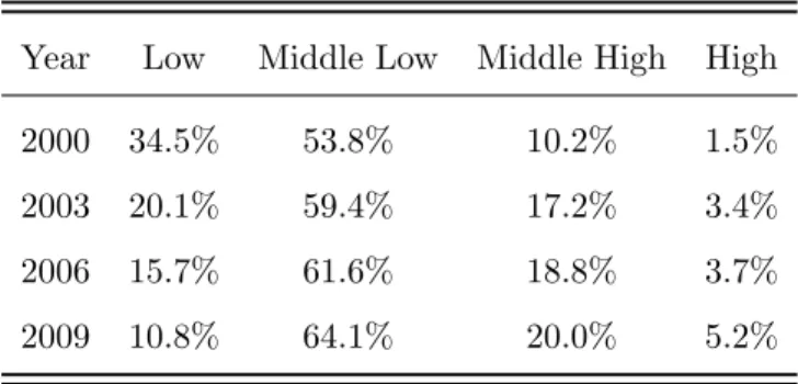
Table 1. in the appendix shows the percentage of private sector workers in the sample per income class in 2000, 2003, 2006 and 2009. It is visible that the composition in 2000 is sightly different from the following years - in 2000 a higher portion of the private sector workers were concentrated in the lower class. Overall, from 2000 to 2009 the concentration of individuals in the bottom part of the distribution seems to have narrowed.
highest share of the private sectors falls into the middle low income class (60%-65%) followed by middle high (17%-20%), low (10%-20%) and high (3%-5%) which is consistent with the definition of classes used by other authors (Piketty 2014)
While the model-based approach allow us to condition on other variables when determining the effect of previous income class, Table 2. in the appendix shows income class dynamics without conditioning on other variables. Each entry in the table can be interpreted as the conditional probabilities under a Markov model. For the most extreme cases, the off-diagonal probabilities of transitions to high/low income class from low/high income class, are almost zero. The high relative magnitudes of the diagonal elements shows the persistence of income class.
Persistence in income class outcomes is clear in both the first (2000-2003) and second (2006-2009) wave. Mobility for the lower class in the second wave seems to have improved when compared to the first wave, while for the remaining classes mobility became more rigid.
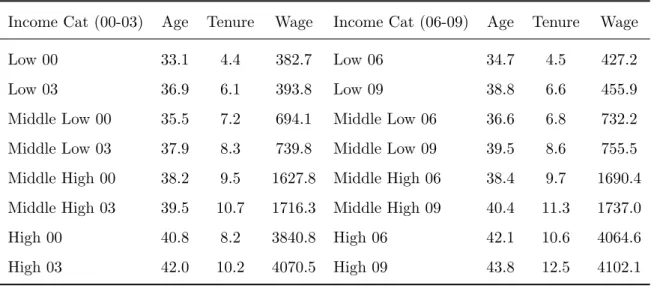
Table 3. in the appendix shows average wage, tenure and age per income class. As expected high income class is associated with a higher average age and tenure. Middle-high income class individuals earn on average 2 times more per month than middle-low class individuals. High income class individuals earn almost 10 times more than low income class individuals, on average.
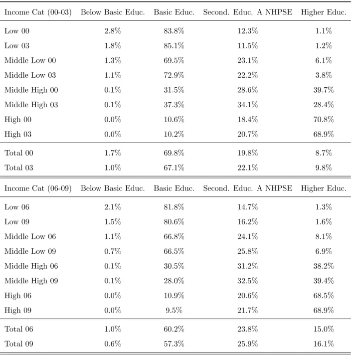
Educational status is usually considered as a determinant of social class and a source of income inequalities. Therefore, it is of interest to consider how income class is related to educational attainment in the Portuguese private sector. Table 5. shows the highest level of education completed by income class. Has expected, lower income classes are associated with basic levels of education and higher income classes are associated with higher levels of educations.15 The share of workers with an education level
below basic is less than 2%. This represents a very small share and for estimation proposes it might be difficult to consider separately this group - it is more feasible to consider a ’Basic education and below’ group.
It is also interesting to look at income class by sex Table 4.. The first thing to notice is that according to the sample of private sector workers there are more men (⇡ 58%) than women in the private labour market. Per year and class, the share of men is higher from the middle low income class up and the proportion of men increases as the income class increases. Around 60% of the low income class are women while around 70% of the high income class are men.
15
There are few cases of low income class workers with higher education, but a part of these are part time working females,
5
Estimation and Results
This section presents the estimation of the probabilities for the income class using the ordered probit models described in section 3. Due to the size and large amount of tables, all the tables are aggregated in Appendix B.
5.1
Ordered probit applications to income mobility, conditional on past status
A simple way to start is by estimating 4 different equations separately conditional on the previous period income class for each wave.
Prob[yt=j|x] =
8 > > > > > > < > > > > > > :
Φ(τj0+1 x0β0) Φ(τ0
j x0β0) if yt 1 = 0
Φ(τj1+1 x0β1)
Φ(τj1 x0β1) if y
t 1 = 1
Φ(τj2+1 x0β2)
Φ(τj2 x0β2) if y
t 1 = 2
Φ(τj3+1 x0β3) Φ(τ3
j x0β3) if yt 1 = 3
The explanatory variables in x include a dummy variable for sex, categorical variables for age and education and tenure (continuous).
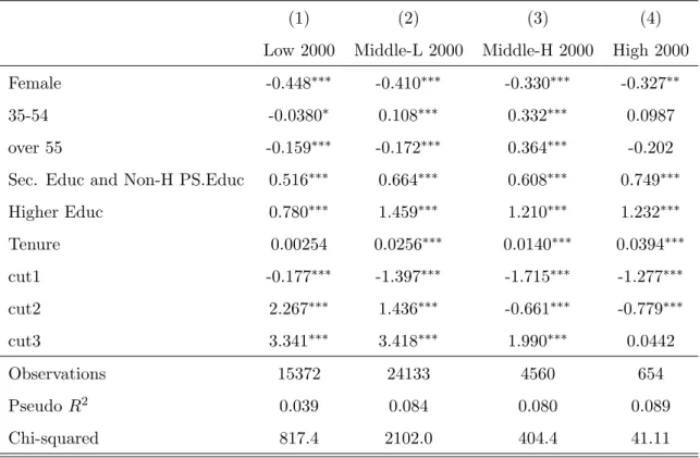
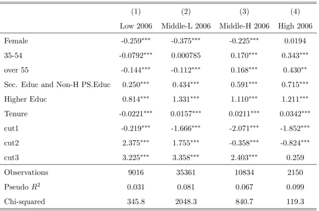
As seen in the previous section the proportion of workers with below basic education was small, particularly in high income class, which makes estimation complicated. Thus, it is more efficient to combine some of the independent variable categories that have low frequencies with adjacent categories. Age will be collapsed into 3 categories (instead of 5): 0 if age is between 16 34, 1 if 35 54 and 2 if 55 or more. Below basic education will be aggregated with basic education, such that the variable education now has also 3 categories. The base group for sex is male. For choosing the right model specification, potential collinearity among explanatory variables was analysed and a LR test was run to check whether the categorical variables could be treated as continuous without loss of information. Other specifications such has age and age squared were also tested (AIC/BIC). The chosen specification is as described above. The results from the estimation for wave 1 and 2 are showed in tables 6 and 7, respectively. The coefficients are significant in most cases, with the exceptions in the first wave being tenure for 2000 low income class and age group for 2000 high income class while in the second wave the ”35-54” bracket is not significant in the 2003 middle-low class and sex in the 2006 high income class.
5.2
Average Predicted Probabilities
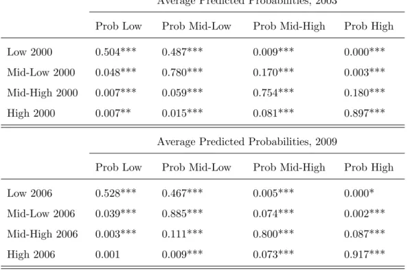
Table 8. in the appendix depicts the average predicted probabilities for 2003 per income class in 2000. Within this wave the high relative magnitudes of the diagonal elements shows the persistence of income class while the off-diagonal shows very few ”extreme” cases. It its interesting the to see that individuals who were low class in 2000 had a relatively high probability of becoming mid-low class in 2003. The predicted probability of going up to the adjacent upper class for the two mid categories is considerably lower than the previous case. High income class workers in 2000 are the ones with the highest probability of remaining in the same class in 2003.
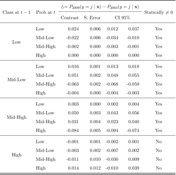
Nevertheless, the focus here is not in the probabilities within the same wave but between waves. We want to test whether the probability of going up the income ladder (given the previous period income class) has changed from the first to the second wave. The test used for analysing the difference in the chances of upward mobility between is has described in 3.3. Recall that we are testing ifM(x) =P(y2009=
j|y2006=s) P(y2003=j|y2000=s) is statistically different from zero (where jands are any of the 4
income classes, alsojcan be =s).
Table 9. gives the differences with confidence intervals. By looking at the first 12 rows it is possible to see that the confidence intervals do not contain zero. Thus we can affirm that for the classes low, mid-low and mid-high int 1 (e.g. 2000 or 2006) the predicted probabilities for being low, low, mid-high or mid-high in t are significantly different between waves at a 5% level. This means for instance, that P(y2009 = Mid-low| x, y2006 = Low) is statistically different from P(y2003 = Mid-low| x, y2000 = Low).
TheM(x) however, is not significant for the cases of high income class int 1, e.g. individuals who where high class in 2006 were as equally likely to remain high class in 2009 as they were in 2000.
The chances of going up in the income ladder for low income class (e.g. the chances to be mid-low, mid-high or high) are lower in 2009 than in 2003. Similarly the chances for mid-low class to be mid-high or high class and the chances for the mid-high class to be high are relatively lower in 2009 than in 2003. The combinations (Low(t) | Low(t 1)), (Mid-low(t) | Mid-low(t 1)) and (Mid-high(t) | Mid-high(t 1)) are statistically higher in 2009 than in 2003. This translates into a higher state persistence in second wave when compared to the first wave.
5.3
Average Marginal E
ff
ects
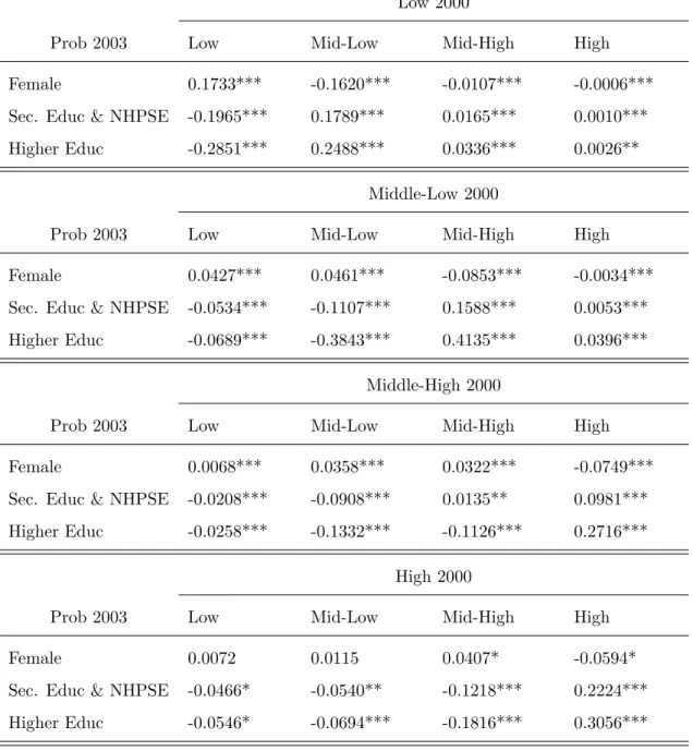
The marginal effects for the first wave show that, on average, females who were low income class are 17.3 percentage points (pp) more likely than males to remain low class in 2003 and 13.6 pp less likely to improve to mid-low class in 2003 (Table 10). Everything else equal, mid-low income class females in 2000 were 4.6 pp more likely to remain mid-class in 2003 than men and less 8.5 pp less likely to become mid-high income class in 2003. Similarly, mid-high class females were 3.2 pp more likely than men to remain in the same class and 7.5 pp less likely than men to become high class. All these results are statistically significant at 1%.
Sex marginal effects results for high income class in the first wave are only significant at 10%. Ac-cordingly, women that were in the high top in 2000 are 5.9 pp less likely to remain high class in 2003 than men and 4.1. pp more likely to come down to mid-high in 2003 than men.
Turning into education, (the base group is ”Basic education or below”) it is expected that individuals who have secondary or higher education are more likely to to improve in social income class (hence positive sign) and less likely to lower their income class (negative sign) than individuals who have only basic education or below. Table 10. shows that this is indeed the case, people with secondary or non-high post secondary education (Sec. Educ & NHPSE) who were low income class in 2000 were 19.7 pp less likely to remain low class in 2003 than people with only basic education or below and 17.9 pp more likely to become mi-low class in 2003. If mid-low income class in 2000, people who attend secondary secondary school were 15.9 pp more likely than basic educated ones to become mid-high class and less 5.3 pp to come down to low class, everything else equal. The results follow for mid-high and high class in 2000. The marginal effects for higher education have the same direction although the magnitude of the effect is considerably larger, as expected.
The results for the second wave follow, in terms of sign, for the great majority of the cases (Table 11.). As seen in the previous sub-section, the effect of sex is not significant for the high income class in 2006 (it was also not significant at 5% in the previous wave).
The results for the marginal effects of tenure and age group for the first wave are showed in Table 12. and for the second wave in Table 13. Broadly speaking belonging to the age group of 35-54 years (relative to 16-34) increases the chances of class improvement for individuals who were middle-low and middle-high in t 1 in both waves. This is not true for low income individuals at t 1. The marginal effect of the highest age group is mixed, but overall it seems to be only positive to mid-high and high classes. The marginal effect of tenure is not significant for thet 1 low income class . The marginal effect of tenure on P(yt = mid-high|yt 1 = mid-low) and P(yt = high|yt 1= mid-high) seems to be positive.
the difference in predicted probabilities) is convenient because it allows us to test just how different are these results between the first and the second using the test described in 3.3. Here the main focus will be on the comparison of the marginal effects on the probability of going up between waves, e.g. focus on P(y= Mid-high|x, y= Mid-low) and not so muchP(y= Low|x, y= Mid-low).
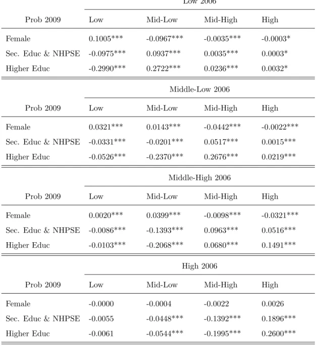
The marginal effect of sex is statistically different between waves for individuals who were low class (Table 14.). Other things being equal, the marginal effect of sex on P(y = Mid-low | x, y = Low), P(y = Mid-high| x, y = Low) and P(y = High| x, y = Low) is stronger in the first wave than in the second. Similarly the marginal effect of sex on theP(y= Mid-high|x, y= Mid-low),P(y= High|x, y= Mid-low) and P(y = High| x, y = Mid-high) is statistically different between waves, being stronger in the first wave. Overall, the effect of gender differences on the probability of moving up in the social class is less pronounced in 2009.
For a matter of space and clear readability Table 15. shows only the results the classes ”above” the class in t 1. The marginal effect for secondary education (base is basic education or below) is statistically different between waves for P(y = Mid-low | x, y = Low) and P(y = Mid-high | x, y = Low) and P(y= High|x, y= Low) although the marginal effect of higher education is not. The marginal effect for both secondary and higher education onP(y= Mid-high|x, y= Mid-low),P(y= High|x, y= Mid-low) and P(y = High | x, y = Mid-high) is statistically different between waves, being stronger in the first wave.
The impact of obtaining a higher level of education (relative to basic education) on the probability of improving in the income class had a stronger impact on first than it had on the second wave.
5.4
A short note on the generalized ordered probit
approach. This might constitute nevertheless a topic for further research.
6
Conclusion
This study proposed the use of an ordered probit model and its extensions to study income mobility in the private sector in Portugal using data from Quadros do Pessoal. The dependent variableywas generated by dividing workers into 4 income classes (low, middle-low, middle-high and high) according to the IRS average tax band their nominal wage would fall into. Worker’s characteristics such as gender, age group, highest educational attainment and tenure were included as explanatory variables.
The workers were separated into two different waves. The first wave is constituted by the same workers observed at 2000 and 2003. The second wave is constituted by the same workers observed at 2006 and 2009. The workers between the two waves are not necessarily the same since the social security number (used to identify the workers) changed in 2005 such that is not possible to match the same workers between waves.
The results from the estimation show that for the classes low, mid-low and mid-high int 1 (e.g. 2000 or 2006) the predicted probabilities of being low, mid-low, mid-high or high intare statistically different between waves at a 5% level. The difference in probabilities however, is not significant for the case of high income class int 1, e.g. individuals who where high class in 2006 were as equally likely to remain high class in 2009 as they were in 2000. Given the negative sign in the difference between probabilities, we can conclude that chances of going up in the income ladder for low, mid-low and mid-high income classes were lower in 2009 than in 2003.
The marginal effects for sex in both waves show that, on average, females who were low, mid-low or mid-high class were more likely than males to remain in the same class and less likely to improve to the adjacent class, everything else equal. Further, the effect of gender differences on the probability of moving up in the social class is less pronounced in 2009 than in 2003. Using ”Basic education or below” as the base group, individuals who have secondary or higher education are more likely to improve in social income class and less likely to lower their income class. than individuals who have only basic education or below in both waves. However, the impact of going from basic education or below to a higher educational level was a stronger determinant of the probability of moving up in the first wave than in the second wave.
to look at the categories of bothyand the x’s and see how theses could possible be re-categorized. The method utilized in this study provides an interesting framework for analysing income class mobility and compare the change in the degree of importance of different social class determinants across time (for instance, if gender inequality has been reduced). This analysis could be even more insightful if the set of explanatory variables was extended. In the QP framework one could match worker’s data with the company data to include informative independent variables such as region and industry, which would allow to analyse other things such as the inequality in the probabilities across regions within Portugal. In a more broad sense it would also be interesting to have explanatory variables that can be directly affected by policy makers such that one can study the impact of certain policies on income class mobility. A deeper analysis of what external factors (affecting the probability of moving up) have change between the waves used in the estimation would also add meaning to the results.
Bibliography
Alesina A. & Perotti, R. (1996). Income distribution, political instability and investment. European Economic Review 40 (6), 1203-1228.
Anderson, G. (2004). Towards an empirical analysis of polarization. Journal of Econometrics 122, 126
Araar, A. (2008). Social Classes, Inequality and Redistributive Policies in Canada, Cahier de recherche/Working Paper 08-17, Centre Interuniversitarire sur le Risque, les Politiques et lEmploi (CIRPEE), Canada.
Atkinson, A. B., Bourguignon, F. (1982). The comparison of multi-dimensioned distributions of economic status. Review of Economic Studies 49 (2), 18320.
Atkinson, A.B.; Bourguignon, F. & C. Morrison (1992). Empirical Studies of Earnings Mobility. Chur, UK: Harwood Academic Publishers).
Atoda N. and Tachibanaki, T.. (1980). Earnings Distribution and Inequality Over Time. Kyoto Institute of Economic Research, Discussion Paper 144.
Atoda N. and Tachibanaki. T. (1991). Earnings Distribution and Inequality Over Time: Education versus, Relative Position and Cohort. International Economic Review 32, 475- 479.
Banerjee, A. & Duflo, E.(2007). What is middle class about the middle classes around the world?. Massachusetts Institute of Technology, Department of Economics, Working Paper No. 07-29.
Barro, R. (1999). Determinants of democracy. Journal of Political Economy, University of Chicago Press, 107(S6), 158-183. Bartholomew, D. J. (1982). Stochastic Models for Social Processes, 3rd Edition. Chichester: Wiley. Bartholomew, D. J. (1996). The Statistical Approach to Social Measurement. San Diego: Academic Press. Blackburn, M. & Bloom, D. (1985). What is Happening to the Middle Class?. American Demographics, vol. 7(1), 19-25.
Birdsall, N.; Graham, C.& Pettinato, St. (2000). Stuck in The Tunnel: Is Globalization Muddling The Middle Class?. Brookings Institution, Center on Social and Economic Dynamics, Working Paper No. 14.
Boes S., Winkelmann R. (2006). Ordered Response Models. Allgemeines Statistisches Archiv, 90 (1) 165-18. Reeditado em : Hbler, O. and J. Frohn (2006) Modern Econometric Analysis, Springer.
Bossert, W. & Schworm, W. (2008), A Class of Two-Group Polarization Measures. Journal of Public Economic Theory 10(6),1169-1187.
Cantante, F. (2012). A magreza da classe mdia em Portugal. Le Monde Diplomatique, Edio Por-tuguesa, Maio de 2012.
Chakravarty, S. R. (2009). Inequality, Polarization and Poverty. Advances in Distributional Analysis, New York: Springer.
of Income and Wealth 56, 4764
Chakravarty, S. R. & Maharaj, B. (2011). Measuring ethnic polarization. Social Choice and Welfare, 37, 431-452.
Chakravarty, S. R. & Majumder, A, (2001). Inequality, polarization and welfare: Theory and appli-cations. Australian Economic Papers 40, 113.
Cruces, G.; Calva, L. F. L. & Battistn, D. (2011). Down and Out or Up and In? Polarization-Based Measures of the Middle Class for Latin America. CEDLAS, Working Papers 0113, CEDLAS, Universidad Nacional de La Plata.
Duclos, J-Y.; Esteban, J. & Ray, D. (2004). Polarization: Concepts, Measurement, Estimation. Econometrica 72(6), 1737-1772.
DAmbrosio, C. (2001). Household Characteristics and the Distribution of Income in Italy: An Appli-cation of Social Distance Measures. Review of Income and Wealth 47, 4364.
DAmbrosio, C.; P. Muliere & Secchi,P. (2002). Income thresholds and income classes. Working Paper, Universita Bocconi, Milano, Italy.
Easterly, W. (2001). The middle-class consensus and economic development. Journal of Economic Growth 6(4), 317-335.
Erikson R, Goldthorpe JH & Portocarero L (1979). Intergenerational class mobility in Three Western Societies: England, France, and Sweden. British Journal of Sociology 30 (4),415441.
Erikson, R. & Goldthorpe, J. H. (1992). The Constant Flux: A Study of Class Mobility in Industrial Societies, Oxford: Clarendon Press.
Erikson, R. & Goldthorpe, J. (2002). Intergenerational inequality: A sociological perspective. The Journal of Economic Perspectives 16, 31-44.
Estanque, E. (2012). A Classe Mdia: Ascenso e Declnio. Lisboa: Fundao Francisco Manuel dos Santos.
Esteban, J. & Ray, D. (1994). On the Measurement of Polarization. Econometrica, 62(4), 819-51. Esteban, J. & Ray, D. (1999). Conflict and Distribution. Journal of Economic Theory 87(2), 379-415. Esteban, J. & Ray, D. (2007). A Comparison of Polarization Measures. UFAE and IAE Working Papers 700.07, Unitat de Fonaments de l’Anlisi Econmica (UAB) and Institut d’Anlisi Econmica (CSIC). Esteban, J. & Ray, D. (2008). Polarization, Fractionalization and Conflict. Journal of Peace Research 45(2), 163-182.
Esteban, J. & Ray, D. (2011). Linking Conflict to Inequality and Polarization. American Economic Review 101(4), 1345-74.
Journal for General Social Issues 17(4-5), 869-886.
Fields, Gary S. & Ok, Efe A. (1996). The Meaning and Measurement of Income Mobility. Journal of Economic Theory 71(2), 349-377.
Fields, Gary S. & Ok, Efe A. (1999). The Meaning and Measurement of Income Mobility. An Introduction to Literature. [Electronic version]. In J. Silber (Ed.) Handbook on income inequality measurement (pp. 557-596). Norwell, MA: Kluwer Academic Publishers.
Foster, J.; Greer, J. & Thorbecke, E. (1984). A class of decomposable poverty measures, Econometrica 52 (3), 761-766.
Foster, J. & Wolfson, M. C. (2010). Polarization and the decline of the middle class: Canada and the U.S.. Journal of Economic Inequality 8(2), 247-273.
Fu, V. (1998). Estimating Generalized Ordered Logit Models. Stata Technical Bulletin, 44, 27-30. Reprinted in Stata Technical Bulletin Reprints, vol. 8, pp. 160164. College Station, TX: Stata Press
Gigliarano, Ch. & Muliere,P. (2012). Measuring Income Polarization Using an Enlarged Middle Class. ECINEQ, Society for the Study of Economic Inequality, Working Papers 271.
Glass, D. V. (1954). Social Mobility in Britain. London: Routledge & Kogan Paul.
Goldthorpe, J. (1980). Social Mobility and Class Structure in Modern Britain. Oxford: Clarendon Press.
Greene, W.H. & Hensher, D.A. (2010). Modeling Ordered Choices: A Primer and Recent Develop-ments, Cambridge: Cambridge University Press.
Jntti, M. & Jenkins, S. P. (2013). Income Mobility. IZA Discussion Papers 7730, Institute for the Study of Labor (IZA).
Jenkins, S.P. (2011). Changing fortunes: income mobility and poverty dynamics in Britain, Oxford: Oxford University Press.
Jenkins, S. P. (2011). Has the instability of personal incomes been increasing? National Institute Economic Review, 218 (1), 33-43.
Jereb, E. & Ferjan, M. (2008). Social classes and social mobility in Slovenia and Europe. Organizacija. Journal of Management, Informatics and Human Resources 41 (6), 197-206.
Lasso de la Vega, C. & Urrutia, A. (2006). An alternative formulation of the Esteban-Gradin-Ray extended measure of bipolarization. Journal of Income Distribution 15, 4254.
Lasso de la Vega, C., Urrutia, A. & Diez, H. (2006). Unit consistency and bipolarization of income distributions. Review of Income and Wealth 56, 6583.
for the Study of Economic Inequality.
Levy, F. (1987). The middle class: Is it really vanishing? The Brookings Review 5, 17-21.
Long, J. S. (1997). Regression Models for Categorical and Limited Dependent Variables. Thousand Oaks, CA: Sage Press.
Long, J.S. (1999). Developments in Quantitative Methodology. In Edgar Borgatta (ed.) Encyclopedia of Sociology.
Long, J.S. (2009). Group comparisons in logit and probit using predicted probabilities, Indiana University, Working Paper, June 25, 2009.
Long, J. S. & Freese, J. (2014). Regression Models for Categorical Dependent Variables Using Stata, 3rd Edition, Stata Press.
Maddala, G. (1983). Limited-Dependent and Qualitative Variables in Econometrics. Cambridge: Cambridge University Press.
Massari, R., Pittau, M. G. & Zelli, R. (2009). A dwindling middle class? Italian evidence in the 2000s. The Journal of Economic Inequality 7, 333350.
McKelvey, R. & W. Zavoina, W. (1975). A Statistical Model for the Analysis of Ordinal Level Variables. Journal of Mathematical Sociology 4,103-120.
Medeiros, M. (2006). The rich and the poor: The construction of an affluence line from the poverty line. Social Indicators Research: An International and Interdisciplinary Journal for Quality-of-Life Mea-surement 78 (1), 1-18.
Milanovic, B. & Yitzhaki, S. (2002). Decomposing World Income Distribution: Does the World Have a Middle Class? Review of Income and Wealth 48(2), 155-178.
Nichols, A. (2007). Causal inference with observational data.The Stata Journal, 7(4): 507541. Nichols, A. (2008). Trends in Income Inequality, Volatility, and Mobility Risk. IRISS, Working Paper 94.
Nichols, A. (2010). Income Inequality, Volatility, and Mobility Risk in China and the US.China Economic Review 21(S1): S3S11.
Nichols, A. & Favreault, M.M. (2009). A Detailed Picture of Intergenerational Transmission of Human Capital. Washington DC: Urban Institute.
Nichols, A. & Rehm, Ph. (2014). Income Risk in 30 Countries. Review of Income and Wealth, 60(S1): S98S116. Pasta, D. J. (2009). Learning When to Be Discrete: Continuous vs. Categorical Predictors. SAS Global Forum 2009, Statistics and Data Analysis, Paper 248.
Piketty, T. (2014). O Capital no sculo XXI. Lisboa: Temas e Debates/Crculo de Leitores
Pittau, M. G.; Zelli, R. & Johnson, P. A. (2010). Mixture models, convergence clubs, and polarization. Review of Income and Wealth 56, 102122.
Prais, S. J. (1955). Measuring social mobility. Journal of the Royal Statistical Society A118, 55-66. Prais, S. J. (1995). Productivity, Education and Training: Facts and Policies in International Per-spective, Cambridge University Press.
Ravallion, M. (2009). The Developing World’s Bulging (but Vulnerable) Middle Class. World Bank Research Working Paper No. 4816.
Shorrocks, A.F. (1976). Income Mobility and the Markov Assumption. Economic Journal 46, 566-578. Shorrocks, A.F. (1978a). The Measurement of Mobility. Econometrica 46 (5), 1013-1024.
Shorrocks, A.F. (1978b). Income Inequality and Income Mobility. Journal of Economic Theory 46, 376-39
Silber, J.; Deutsch, J. & Hanoka, M. (2007). On the link between the concepts of kurtosis and bipolarization. Economics Bulletin 4, 1-6.
Solimano, A. (2008). The Middle Class and the Development Process. Macroeconomia del Desarrollo / Macroeconomic of Development series, No. 11, Economic Commission for Latin America and the Caribbean (ECLAC).
Sommers, P. M. & Conlisk, J. (1979). Eigenvalue immobility measures for Markov chains. Journal of Mathematical Sociology, 6, 25376.
Terza, J. (1985). Ordered Probit: A Generalization. Communications in Statistics A. Theory and Methods 14, 111.
Torche, F. & Lopez-Calva, L. F. (2010). Stability and vulnerability of the Latin American middle class. In: Newman, K. (ed.), Dilemmas of the Middle Class Around the World, Oxford University Press. Wang, Y. and Tsui, K. (2000). Polarization orderings and new classes of polarization indices. Journal of Public Economic Theory 2, 349363.
Williams, R. (2006). Generalized ordered logit/partial proportional odds models for ordinal dependent variables. The Stata Journal 6 (1), 58-82.
Williams, R. (2010). Fitting heterogeneous choice models with oglm. The Stata Journal 10 (4), 540-567.
Williams, R. (2016). Understanding and interpreting generalized ordered logit models. The Journal of Mathematical Sociology 40 (1), 7-20.
Wolfson, M. C. (1994). When inequalities diverge. The American Economic Review 84, 353358. Wolfson, M. C. (1997). ’Divergent inequalities: Theory and empirical results’. Review of Income and Wealth 43, 401421.
World Bank (2007). Global Economic Prospects: Managing the Next Wave of Globalization, Wash-ington DC: World Bank.
Yitzhaki, S. (2010). Is there room for polarization?. Review of Income and Wealth 56, 722.
A
Appendices
A.1
Data treatment and analysis
A.1.1 Tax Band Notes
For instance, based on the 2006 average income tax bands for single individuals (Ministry of Social Security) one can divide the income tax bands into 4 groups:
• Up to 4,451 euros a year pays an average tax rate of 10.50% (Low income class)
• From 4,351 to 6,732 euros a year pays an average tax rate of 11.35% (Low income class)
• From 6,732 to 16,692 euros a year pays an average tax rate of 18.60% (Middle-Low income class)
• From 16,692 to 38,391 euros a year pays an average tax rate of 27.30% (Middle-high income class)
• From 38,391 to 55,639 euros a year pays an average tax rate of 30.15% (High income class)
• Above 55,639 euros a year pays an average tax rate of 30.87% (High income class)
Tax bands change slightly from year to year because of inflation and in some cases because of changes to the bands themselves. Therefore for the same wave incomes and tax bands are deflated to a common year (2006). Furthermore, all the wage data from 2000 was converted from escudos to euros using the exchange rate established by the Central Bank at the time of the transition (1 euro = 200,482 escudos).
A.1.2 Statistics
Year Low Middle Low Middle High High
2000 34.5% 53.8% 10.2% 1.5% 2003 20.1% 59.4% 17.2% 3.4% 2006 15.7% 61.6% 18.8% 3.7% 2009 10.8% 64.1% 20.0% 5.2%
Income Category in 2003
Income Cat in 2000 Low Middle Low Middle High High
Low 86.9% 28.2% 1.9% 0.5% Middle Low 12.7% 70.7% 53.0% 5.2% Middle High 0.4% 1.0% 44.4% 54.7% High 0.1% 0.0% 0.7% 39.6%
Income Category in 2009
Income Cat 2006 Low Middle Low Middle High High
Low 77.4% 11.6% 0.4% 0.1% Middle Low 22.2% 85.1% 23.1% 2.5% Middle High 0.4% 3.3% 75.1% 31.2% High 0.0% 0.1% 1.4% 66.2%
Table 2: Income class transition matrices
Income Cat (00-03) Age Tenure Wage Income Cat (06-09) Age Tenure Wage
Low 00 33.1 4.4 382.7 Low 06 34.7 4.5 427.2 Low 03 36.9 6.1 393.8 Low 09 38.8 6.6 455.9 Middle Low 00 35.5 7.2 694.1 Middle Low 06 36.6 6.8 732.2 Middle Low 03 37.9 8.3 739.8 Middle Low 09 39.5 8.6 755.5 Middle High 00 38.2 9.5 1627.8 Middle High 06 38.4 9.7 1690.4 Middle High 03 39.5 10.7 1716.3 Middle High 09 40.4 11.3 1737.0 High 00 40.8 8.2 3840.8 High 06 42.1 10.6 4064.6 High 03 42.0 10.2 4070.5 High 09 43.8 12.5 4102.1
Income Cat (00-03) Female Male Income Cat (06-09) Female Male
Low 00 58.5% 41.5% Low 06 61.5% 38.5% Low 03 63.1% 36.9% Low 09 62.7% 37.3% Middle Low 00 34.0% 66.0% Middle Low 06 40.4% 59.6% Middle Low 03 39.0% 61.0% Middle Low 09 41.9% 58.1% Middle High 00 29.1% 70.9% Middle High 06 33.8% 66.2% Middle High 03 30.2% 69.8% Middle High 09 35.0% 65.0% High 00 18.1% 82.0% High 06 23.1% 76.9% High 03 21.2% 78.8% High 09 24.7% 75.3%
Total 00 41.8% 58.2% Total 06 41.9% 58.1% Total 03 41.8% 58.21% Total 09 41.9% 58.1%
Income Cat (00-03) Below Basic Educ. Basic Educ. Second. Educ. A NHPSE Higher Educ.
Low 00 2.8% 83.8% 12.3% 1.1%
Low 03 1.8% 85.1% 11.5% 1.2%
Middle Low 00 1.3% 69.5% 23.1% 6.1% Middle Low 03 1.1% 72.9% 22.2% 3.8% Middle High 00 0.1% 31.5% 28.6% 39.7% Middle High 03 0.1% 37.3% 34.1% 28.4%
High 00 0.0% 10.6% 18.4% 70.8%
High 03 0.0% 10.2% 20.7% 68.9%
Total 00 1.7% 69.8% 19.8% 8.7%
Total 03 1.0% 67.1% 22.1% 9.8%
Income Cat (06-09) Below Basic Educ. Basic Educ. Second. Educ. A NHPSE Higher Educ.
Low 06 2.1% 81.8% 14.7% 1.3%
Low 09 1.5% 80.6% 16.2% 1.6%
Middle Low 06 1.1% 66.8% 24.1% 8.1% Middle Low 09 0.7% 66.5% 25.8% 6.9% Middle High 06 0.1% 30.5% 31.2% 38.2% Middle High 09 0.1% 28.0% 32.5% 39.4%
High 06 0.0% 10.9% 20.6% 68.5%
High 09 0.0% 9.5% 21.7% 68.9%
Total 06 1.0% 60.2% 23.8% 15.0%
Total 09 0.6% 57.3% 25.9% 16.1%
Note: NHPSC refers to Non-high post secondary education
A.2
Estimation Results Tables
A.2.1 Ordered probit regression output
(1) (2) (3) (4)
Low 2000 Middle-L 2000 Middle-H 2000 High 2000 Female -0.448⇤⇤⇤ -0.410⇤⇤⇤ -0.330⇤⇤⇤ -0.327⇤⇤
35-54 -0.0380⇤ 0.108⇤⇤⇤ 0.332⇤⇤⇤ 0.0987
over 55 -0.159⇤⇤⇤ -0.172⇤⇤⇤ 0.364⇤⇤⇤ -0.202
Sec. Educ and Non-H PS.Educ 0.516⇤⇤⇤ 0.664⇤⇤⇤ 0.608⇤⇤⇤ 0.749⇤⇤⇤
Higher Educ 0.780⇤⇤⇤ 1.459⇤⇤⇤ 1.210⇤⇤⇤ 1.232⇤⇤⇤
Tenure 0.00254 0.0256⇤⇤⇤ 0.0140⇤⇤⇤ 0.0394⇤⇤⇤
cut1 -0.177⇤⇤⇤ -1.397⇤⇤⇤ -1.715⇤⇤⇤ -1.277⇤⇤⇤
cut2 2.267⇤⇤⇤ 1.436⇤⇤⇤ -0.661⇤⇤⇤ -0.779⇤⇤⇤
cut3 3.341⇤⇤⇤ 3.418⇤⇤⇤ 1.990⇤⇤⇤ 0.0442
Observations 15372 24133 4560 654 Pseudo R2 0.039 0.084 0.080 0.089
Chi-squared 817.4 2102.0 404.4 41.11
⇤p <0.10,⇤⇤p <0.05,⇤⇤⇤p <0.01