Rate-Distortion Analysis for
H.264/AVC Video Statistics
Luis Teixeira
Research Center for Science and Technology in Art (CITAR),
School of Arts, Portuguese Catholics University,
INESC PORTO – Instituto Nacional de Engenharia de Sistemas e Computadores
Portugal
1. Introduction
MPEG standards family specify the decoding process and the bit-stream syntaxes allowing research towards the optimizations of the encoding process regarding coding performance improvement and complexity reduction. The purpose of a video encoder for broadcast or storage is to generate the optimal perceptual video quality, or the minimized distortion, under a certain constraint such as storage space or channel bandwidth. In particular, by minimizing the distortion D, the video encoder should optimally compute a set of optimal quantisers to control the output bit-rate for each coding unit to satisfy the allocated bit budget.
There are two main approaches to solve the optimal bit allocation problem: Lagrange optimization (Everett, 1963; Ramchandran et al., 1994) and dynamic programming (DP) (Bellman, 2003). The optimal bit allocation was first addressed in (Huang & Schultheiss, 1963) where the Lagrange multiplier approach for R-D analysis in transform coding was used. Further improvements have been reported in (Shoham & Gersho, 1988) for source quantization and coding. However, the Lagrange multiplier method suffer from problems, such as having negative bits and real numbers (Schuster & Katsaggelos, 1997a) and the computational complexity is very high due to the need to determine R-D characteristics of current and future video frames. DP is employed to achieve the minimum overall distortion through a tree or trellis with known quantisers and their R-D characteristics (Forney, 1973; Ortega, 1996; Ramchandran et al., 1994).
The total of the required bits and coding distortion depend on the quantization step-size. The rate or distortion versus quantization parameter (Q) curve can be produce by encoding for all the possible quantisers to obtain the bit-rate and the quantization error. In order to know how to select a quantization parameter under a specific constraint, e.g., the target bit-budget or distortion, it is importance to model or estimate the coding bit rate in terms of the quantization parameter, namely rate-quantization (R-Q) functions. Together with distortion-quantization (D-Q) functions, R-Q functions characterize the rate-distortion (R-D) behaviour of video encoding, which is the key to obtain an optimum bit allocation. Many R-Q and D-Q functions have been reported in previous studies (Chiang & Zhang, 1997; Ding & Liu, 1996; Hang & J.J. Chen, 1997; ISO/IEC, 1993; ISO/IEC, 1997; ITU-T, 1997; Lin & Ortega, 1998;
Ortega, 1996; Ribas-Corbera & Lei, 1999; Sullivan & Wiegand, 1998; Yin & Boyce, 2004). Some of these schemes were adopted in standard-compliant video coders, such as TM-5 (ISO/IEC, 1993), the test model for MPEG-2, TMN-8 (ITU-T, 1997), the test model for H.263, and VM-8 (ISO/IEC, 1997), the verification model for MPEG-4.
Usually rate control algorithms accept as an assumption that video source statistics are stationary. In this case, video source statistics correspond to some form of probability model such as Gaussian (Hang & J.J. Chen, 1997) or Laplacian (Chiang & Zhang, 1997) and R-D models based on the R-D theory, the theoretical foundation of rate control, can be obtained (Berger, 1971; Chiang & Zhang, 1997; Ribas-Corbera & Lei, 1999).
A video coding algorithm focus on the trade-off between the distortion and bit rate, where usually to a decreasing distortion corresponds an increasing rate and vice-versa. In R-D theory, the R-D function allows to estimate the lower bound for the rate at a given distortion. However, this value may not be possible to obtain in practical video encoders implementations. Operational R-D (ORD) theory applies to lossy data compression with finite number of possible R-D pairs (Schuster & Katsaggelos, 1997a).
Rate
Operational Rate-Distortion
Rate Distortion Model
Distortion Fig. 1. Operational rate-distortion and rate-distortion model curves.
The ORD function presents the convex curve of the specific compression scheme such that the optimal solution of rate control, i.e., optimal quantiser achieving minimum distortion at given bit rate, can be obtained (Schuster& Katsaggelos, 1997a) (Figure 1). Efficiency problems in many practical video coding applications may occur due to high computational complexity in this approach (Z. Chen & Ngan, 2007). Therefore, in numerous systems, model-based rate control schemes have been adopted (Chiang & Zhang, 1997; Ding& Liu, 1996; Vetro et al., 1999; Z. Chen & Ngan, 2005a; Zhang et al., 2005). R-D models can be obtained based on the statistical properties of video signal and R-D theory (Chiang & Zhang, 1997; Hang & J.J. Chen, 1997; Ribas-Corbera & Lei, 1999), or on empirical observation and benefiting from various regression techniques (Ding& Liu, 1996; Kim, 2003; Lin & Ortega, 1998; Z. Chen & Ngan, 2004; Z. Chen & Ngan, 2005b).
Some rate control schemes incorporate spatio-temporal correlations to improve the accuracy of R-D models, by using statistical regress analysis for dynamical model parameters update. Representative of this approach is the MPEG-4 Q2 (Chiang & Zhang, 1997), and the linear MAD models (Lee et al., 2000), where model parameters are updated by linear regression method from previous coded parameters. H.264/AVC JM rate-control algorithm also uses a quadratic rate model. In addition, the H.264/AVC rate-control solves “chicken-and-egg” dilemma as the Lagrange multiplier is modelled as a function of quantization parameter (Wiegand & Girod, 2001). Rate-quantization relationship can be used to compute the quantization parameter. Nevertheless, the model-based rate functions frequently depend on the complexity of the coding unit that is obtained after the rate-constrained motion estimation and mode decision with the Lagrange multiplier. The JM algorithm of H.264/AVC proposes a linear prediction model to solve this problem by estimating the mean of absolute difference (MAD) from the previously coded units. Then the quadratic model can estimate the quantization parameter. However, rate-distortion re-analysis can be further investigated based on the coding characteristics of the H.264/AVC for improving the coding performance (Kamaci et al., 2005; Ma et al., 2005) particularly in the case of joint video coding and the use of different distortion metrics.
We may find in the literature extensive studies regarding optimizing a video encoder encoder with R-D considerations include mode decision (Chan & Siu, 2001; Chung & Chang, 2003), motion estimation (Pur et al., 1987; Rhee et al., 2001; Wiegand et al., 2003b), optimal bit allocation and rate control in video coding field (H.-Y.C. Tourapis & A.M. Tourapis, 2003; He & Mitra, 2002; J.J. Chen & Lin 1996; Ortega, 1996; Ramchandran et al., 1994; Ribas-Corbera & Neuhoff, 1998; Schuster& Katsaggelos, 1997b; Sullivan & Wiegand, 1997; Wiegand et al., 2003a, 2003c; Zhang et al., 2003).
In summary, to optimize a video encoder, the rate-distortion optimization techniques play a very important role. R-D models are functions that predict the expected distortion at a given bit rate. This is very important for joint video coding applications that attempt to optimized quality, e.g. minimize distortion, in environments where the channel conditions vary dynamically or the number of broadcast programs varies through time. Thus in this section we propose to present and evaluate several R-D models.
At the same time, we propose also to study the bit rate variability as a function of the video quality (Seeling et al., 2004, 2007). This type of analyse is typical of a communication network perspective. By re-analyzing the characteristics of the bit-rate and the data in the transform domain, a simple rate estimation function can be obtained that will allow support the allocating of video bandwidth within different video programmes.
2. Rate control in international standards
Although the MPEG video coding standard recommended a general coding methodology and syntax for the creation of a legitimate MPEG bitstream, there are many areas of research left open regarding how to generate high-quality MPEG bitstreams. This allows the designers of MPEG encoder great flexibility in developing and implementing their own MPEG specific algorithms. To optimise the performance-of an MPEG encoder system, it is important to study research areas such as motion estimation, coding mode decisions, and rate control.
The main goal of rate control is to manage the process of bit allocation within a video sequence and thus the quality of the encoded bitstream. Regarding rate control, encoders
can operate at Constant Bit Rate (CBR) or in Variable Bit Rate (VBR). In CBR, the video encoder maintains the average bit rate constant. The encoder output has a buffer and its occupancy is controlled dynamically by adjusting the quantization scale, denote as q in MPEG coders. Likewise, the quality of the video sequence varies due to the variations in the scene complexity. VBR reduces the variation in the picture quality by allocating more bits to complex images. A common use of VBR is Open-Loop Variable Bit Rate (OL-VBR), where the quantization scale is constant for all the images of the video sequence. Another VBR scheme is Constant Quality - Variable Bit Rate (CQ-VBR) which aims to maintain an objective video quality constant.
The rate control algorithms usually adjust the coded bit stream according different constraints, such as buffer over- or underflow prevention, variable and/or low bandwidth constraints resulting from limited storage size or communication bandwidth (Ortega, 1996). In order to accomplish this goal rate control schemes are responsible to adjust the quantization parameters. Video Encoder Rate Control Encoder Buffer Bitstream Video Source
Fig. 2. Rate control in video coding system.
A generic bit rate control is composed the following steps: given an input video signal and a desired bit rate, constant or variable, what should be the encoder settings to maintain the picture quality as high and constant as possible. In MPEG encoding, a quantization scale controls the trade-off between picture quality and the bit rate. This parameter is used to compute the step size of the uniform quantisers used for the different AC DCT coefficients (ISO/IEC, 1993). For each macroblock, a quantiser, q, is selected. It is named “adaptive quantization” to the process for adjusting the value of q between macroblocks within an image frame. There are several schemes for doing the adaptive quantization. For example, in MPEG-2 Test Model 5 (TM5) (ISO/IEC, 1993), a non-linear mapping based on the block variance is used to adapt the q's. Besides the quantization scale, the quantization coarseness is also dependent of the quantization matrix. In MPEG-1, the quantization matrix can be altered in each sequence while in MPEG-2 on a picture basis. It sets the relative coarseness of quantization for each coefficient.
As MPEG does not specify how to control the bit rate, different approaches can be found in the literature (ISO/IEC, 1993; Keesman et al., 1995; Ramchandran et al., 1993). Two approaches have been used: ‘feed forward bit rate control’ and ‘feed backward bit rate control’. In the first approach, after performing a pre-analysis, the optimum settings are compute. This process will increase the computational complexity and time needed while yielding better results. In the second approach, there is limited knowledge of the sequence complexity. Bits are allocated on a picture basis and spatially uniform distributed throughout the image. Thus, too many bits may be spent at the beginning of the picture while the end of the picture may present a higher degree of complexity. The ‘feed backward bit rate control’ is suitable for real time applications and ‘feed forward bit rate control’ for applications where the quality is the main goal and time is not a constraint.
3. Rate control in H.264/AVC
Existing studies indicate that H.264/AVC brings major improvement in coding performance in relation to prior coding standards (Wiegand et al., 2003a). H.264/AVC presents many new features, which represent huge challenges to the operative encoder control such as how to allocate the bandwidth between the texture coding and the overhead coding.
A major contributor to the high coding efficiency of H.264/AVC compared with previous video compression standards is the rate and distortion (R-D) optimized motion estimation and mode decision (also referred to as RDO) with various intra and inter prediction modes and multiple reference frames. Nevertheless, these innovations increase the rate control process complexity due to the inter-dependency between the RDO and rate control. Only after the end of intra/inters prediction, the rate control scheme can access the exact coding characteristics. This information is necessary for the computation of the quantization parameter. Such a dilemma prevents the rate control scheme from directly accessing the coding characteristic in advance. The dilemma of selecting which parameter should be first determine is sometimes referred in the literature as to the “chicken and egg” dilemma (Li et al., 2003c, 2004; Wu et al., 2005).
To avoid this dilemma, in JVT-D030 a two-pass scheme was proposed, where in each pass a TM-5-alike method was used (Ma et al., 2002). This approach uses an extremely simplified R-D function, which fails to achieve accurate and robust rate control and due to the two-pass increase the level of complexity. Because of these drawbacks, JVT-G012 (Li et al., 2003a) was proposed and accepted as the standardized rate control scheme for H.264/AVC. In JVT-G012, a linear MAD model predicts the coding complexity, and a MPEG-4 Q2 function employed to estimate the quantization parameter (Li et al., 2003a).
First step occurs at GOP level. This step estimates the bits available for the remaining frames in the GOP. In addition, it initializes the QP of instantaneous decoding refresh (IDR) frame. In the following step, rate control algorithm operates at Picture level: an estimation of the target bits for the current basic unit is determined. A basic unit is a group of macroblocks and its size can vary from one macroblock up to the entire picture. The target bits estimation should be allocate so that a similar number of bits are allocate for every picture and the target buffer level is preserve.
The next step is, based on the number of bits used to encode the previous basic units, to estimate the necessary bits to encode the header. The target texture is obtained by subtracting the header estimation to the total target bits estimate. After that, this value is converted to a target QP value using a quadratic model that correlates the QP with the texture bits. The quadratic model needs an estimation of the MAD of the motion-compensated or intra prediction error of the current basic unit’s. Consequently, the rate control model requires an additional linear MAD model that, from the previous basic unit MAD, allows the computation of the current basic unit MAD. In summary, the Picture level process consist in computing the quantization step Qstep using a quadratic model and then performing a R-D optimization (RDO) (Wiegand et al., 2003a) for each MB in the frame. The MAD of the current stored picture, , is predicted by a linear regression method similar to that of MPEG-4 Q2 after coding each picture or each basic unit (1) using the actual MAD of the previous stored picture,
i(j 1 L)1 2
( ) ( 1 )
i j a i j L a
where a1 and a2 are the model parameters (first-order and second-order coefficients). The initial value of a1 and a2 are set to one and zero, respectively (Lim et al., 2007). The quantization step corresponding to the target bits is computed by the equation (2)
1 2 2 , , , ( ) ( ) ( ) ( ) ( ) ( ) i i i h i step i step i j j T j c c m j Q j Q j
(2)where mh,i(j) is the total number of header bits and motion vector bits, c1 and c2 are two
coefficients. The corresponding quantization parameter QPi(j) is computed by using the relationship between the quantization step and the quantization parameter of AVC (Lim et al., 2007). Final step consists in updating the quadratic QP/bits linear model and the MAD model. This process repeats for each basic unit until the complete video sequence has been encoded.
In this section, it was introduce the basis of rate control architecture in JM H.264/AVC (Lim et al., 2007). More detail information is available at (Li et al., 2003b , 2003c , 2004; Lim et al., 2007; Ma et al., 2002). Other solutions can be found in the literature. For example, Zhihai He (He, 2001) has proposed a new model that achieves a good performance for H.263 and MPEG4-2 (ISO/IEC 14496-2) codecs. The parameter ρ represents the percentage of zeros among the quantized transform coefficients. He found a linear relationship between the value ρ and the real bit rate because the percentage of zeros plays an important role in determining the final bit rate
4. Test video sequences
Selecting a representative set of video sequences is a crucial step in evaluating and analysing the performance of R-D models. A homogeneous set of video sequences may generate biased comparison results, because some models may perform especially well under certain sequences. Two key features are used to characterize video sequences: spatial complexity and temporal complexity. Usually, spatial complexity is measured by averaging all neighbourhood differences in the same frame while temporal complexity is measured by averaging neighbourhood differences between adjacent frames (Adjeroh & Lee, 2004). The set of test video sequences is composed by twelve CIF video sequences, with the duration of 10 seconds that are known as test video sequences (ITU-T, 2005).
It were included sequences with low spatial and temporal complexity (low complexity sequences) up to sequences with high spatial and temporal complexity (high complexity sequences). Sequences that have either high spatial or temporal complexity but nor both the designated them as medium-complexity sequences. It follows a brief description of the sequences.
In seven video sequences, the position of the camera is fixed: Akiyo (aki), Deadline (dea), Hall (hal), Mother and Daughter (mad), News (new), Paris (par) and Silence (sil). In the Akiyo sequence, the camera is focus on a human subject with a synthetic background (a female anchor reading the news). The movements are very limited, mainly head movements in front of a fixed camera. In Deadline, Mother and Daughter and Paris sequences, the camera is still fixed but there are more movements of the bodies and heads. These are typical videoconferencing content. In the News sequence two reporters, a male and a female anchor, reading the news in front of a fixed camera in a newsroom while in the background, two dancers execute movements. Hall sequence is an example of a video supervision, with stationary camera and two moving persons: one people entering from the left with a
briefcase and then leaving the hall. In the middle of the sequence, a second person enters the hall from the right and then grabs a monitor. In the Silence sequence, one can observe a fast moving subject executing deaf gesture language.
(a) Akiyo (b) Coastguard (c) Deadlined (d) Flower Garden
(e) Football (f) Foreman (g) Hall (h) Mobile & Calendar
(i) News (j) Paris (k) Silence (l) Mother & Daughter Fig. 3. Video test sequences
The Foreman sequence (for) contain the head of a person talking and geometric shapes. Fast camera movement and content motion with a pan to a construction site at the end characterize this sequence. The main characteristics of the Flower Garden sequence (flg) is the slow and steady camera panning over landscape over landscape; the spatial and the colour detail. Coastguard sequence (cgd) was shot as a pan from left to right movement in the first third and a pan from left to right in the rest of the sequence. The camera movement follows the movements of two boats (the first from right to left and the second movement from left to right). The Mobile and Calendar (mcl) sequence is characterized by the slow panning and zooming of the camera, complex motion; high spatial and colour detail. Fast and complex motion movements of the camera and contents and the level of detail characterize the Football sequence (fot). This is a very diverse set of video sequences
5. Experimental setup
Simulations were performed with the JM reference software, the official MPEG and ITU reference implementation, for the H.264/AVC Main profile (ITU-T, 2005). Source code was compiled with Microsoft Visual C++:
GOP Pattern IntraPeriod Number of B Frames Pattern IBBP_GOP1 10 2 IBBPBBPBBPBBPBBPBBPBBPBBPBBPBB IBBP_GOP2 4 2 IBBPBBPBBPBB IPPP_GOP1 4 0 IPPP IPPP_GOP2 10 0 IPPPPPPPPP
Table 1. Evaluated GOP Patterns
Four different type of GOP patterns were used (Table 1). A typical GOP pattern (IBBP_GOP2), an “extend” B frame version of the typical GOP pattern, and two GOP patterns without Interpolated images.
Additionally, each video test sequence was encoded in two modes: Open-loop (fixed QP with values ranging from 10 up to 42) and Constant Bit Rate (Fixed Rate - 64kbps, 128kbps, 256kbps, 384kbps, 512kbps, 640kbps, 768kbps, 1024kbps, 1536kbps, 2048kbps. The goal was to obtain sufficient data to obtain R-D curves.
Typical quality metrics include Peak signal-to-noise ratio (PSNR) and the Mean Square Error (MSE), Sum of Squared Differences (SSD), Mean Absolute Difference (MAD), and Sum of Absolute Differences (SAD).
2 10 255 10 log PSNR MSE (3) 1 MSE SSD HW (4)
2 1 1 0 0 ˆ , , H W x y SSD p x y p x y
(5) 1 MAD SAD HW (6)
1 1 0 0 ˆ , , H W x y SAD p x y p x y
(7)where H and W are the height and the width of the image frame, and p(x, y) and p x yˆ
,represent the “original” and the reconstructed image frame pixels at (x, y).
Complementary with the study of rate-distortion performance it is propose to include an analysis of the bit rate variability as a function of the video quality. This is an important topic when considering multimedia traffic. The bit rate variability is usually characterized by the Coefficient of Variation (CoV) of the frame sizes (in bits), whereby the CoV is defined as the standard deviation of the frame sizes normalized by their mean X (Seeling et al., 2004, 2007)
CoV X
(8)
1 1 M m m X X M
(9)and the variance
2 (square of the standard deviation) of the frame sizes being defined as
2 2 1 1 ( 1) M m m X X M
(10)6. Experimental results and discussion
This section presents experimental results: Rate-Distortion analysis and bit rate variability analysis as a function of the video quality.
6.1 R-D models
The RD graphs obtained for the video sequences Akiyo, Foreman and Football, in open loop, are show in Figure 4 (bit-rate axe is in logarithm scale). One can observe that a proportional relation exists between Bit-rate and Picture Quality and that quality depend on the video nature: for the same bit-rate, low complexity sequences present higher values of quality and vice-versa. This behaviour occurs in all the different GOP patterns. Figure 5
present graphic representation for RD data in Constant Bit Rate for the same three video sequences using JM rate control. In this case a relation between bit rate and quality can be observed.
Fig. 5. Rate-distortion curve (Akiyo, Foreman, Football; FixeRate)
Frequently data can be noisy in its nature. Thus recognizing the trends in the data is important (Vardeman, 1994). One of the available methods for data analysis and identify existing trends in physical systems is curve fitting. The concept of curve fitting is rather simple: to use a simple function to describe a trend by minimizing the error between the selected function to fit and a set of data (Vardeman, 1994). The principle of least squares is applied to the fitting of a line to (x, y) data. Representative work for estimate the quantization step size has been most direct towards developing all kinds of rate-quantization (R-Q) models like polynomial (including linear and quadratic) (Chiang & Zhang, 1997; Lin & Ortega, 1998; Ronda et al., 1999; Yan & Liou, 1997), spline ( Lin et al., 1996), logarithmic (Ding& Liu, 1996; Hang & J.J. Chen, 1997), power (Ding& Liu, 1996), etc. Yang et al. (Kyeong Ho Yang at al, 1997) proposed a more complex model that combines a logarithmic and a quadratic model. Most of the models only consider the rate function, and often implicitly assume that the distortion is a linear function of the quantization scale. This work has been extended to include D(QP) implementing several methods in order to compare their results. In fact, the goal is to model the quality versus quantization step
relationship and then to evaluate the different approaches to quality metric. It is presume that there is an inverse relationship between quality and distortion.
Before fitting data into a function that models the relationship between two measured quantities, it is a normal procedure to determine if a relationship exists between these quantities. It was decide to use the correlation method to confirm the degree of probability that a relationship exists between two measured quantities (Vardeman, 1994). In the case of no correlation between the two quantities, then there is no tendency for the values of one quantity to increase or decrease with the values of the second quantity. To evaluate the quality of the fit, it is used the sample correlation that represents the normalized measure of the strength of linear relationship between variables (Vardeman, 1994):
T T T x y r x x y y (11)
2 2 2 2 2 2 i i i i i i i i i i i i x y x y x x y y n r x y x x y y x y n n
(12)where r is a matrix of correlation coefficients (Vardeman, 1994). The sample correlation always lies in the interval from -1 to 1. A value of r near of positive one or negative one, it is interpreted as indicating a relatively strong relationship and r near zero is inferred as indicating a lack of relationship. The sign of r indicates whether y tends to increase or decrease with increase x.
IBBP-GOP1 IBBP-GOP2
Sequence I Type P Type B Type I Type P Type B Type Aki 0.8380 0.8470 0,9016 0,8645 0,8447 0,9034 Cgd 0.9210 0.9136 0,9595 0,9180 0,9139 0,9609 Dea 0.8853 0.8909 0,9303 0,8943 0,8878 0,9318 Flg 0.9137 0.9035 0,9349 0,9147 0,8962 0,9342 For 0.8964 0.8881 0,9197 0,8968 0,8836 0,9197 Fot 0.9588 0.9557 0,9691 0,9567 0,9550 0,9695 Hal 0.8154 0.7972 0,8589 0,8003 0,7936 0,8628 Mad 0.8797 0.8666 0,9124 0,8653 0,8645 0,9129 New 0.9554 0.9081 0,9511 0,9091 0,9128 0,9524 Par 0.9455 0.9435 0,9638 0,9461 0,9434 0,9651 Sil 0.9451 0.9412 0,9567 0,9419 0,9421 0,9576 Mcl 0.9356 0.9272 0,9470 0,9329 0,9250 0.9488 Table 2. Correlation coefficients between Bits Frames and Quality Metric (PSNR) for different H.264/AVC video sequences (IBBP-GOP1 and IBBP-GOP2).
IPPP – GOP1 IPPP – GOP2 Sequence I Type P Type I Type P Type Aki 0.8962 0.9170 0.9107 0.9065 Cgd 0.9608 0.9617 0.9615 0.9609 Dea 0.9304 0.9406 0.9354 0.9348 Flg 0.9555 0.9586 0.9567 0.9572 For 0.9268 0.9333 0.9326 0.9289 Fot 0.9659 0.9686 0.9649 0.9665 Hal 0.8540 0.8848 0.8598 0.8646 Mad 0.9019 0.9200 0.9225 0.9121 New 0.9353 0.9492 0.9526 0.9391 Par 0.9609 0.9668 0.9627 0.9630 Sil 0.9605 0.9662 0.9613 0.9621 Mcl 0.9584 0.9715 0.9615 0.9636
Table 3. Correlation coefficients between Bits Frames and Quality Metric (PSNR) for different H.264/AVC video sequences (IPPP-GOP1 and IPPP-GOP2).
Equation (12) was computed for all the twelve sequences, and results were obtained according the different Picture Type and GOP pattern (Table 2 and Table 3). Thus, it was assess the hypothesis of a relationship between PSNR and Rate. Results are very high, for all the video sequences and GOP patterns, near positive one, pointing clearly to a strong positive linear relationship evident. Next step is thus to select what curve fitting functions should be assessed. Due to its simplicity, the first selected is one of the most commonly used techniques: the fitting of a straight line to a set of bivariate data generating a linear equation such as (13) (Vardeman, 1994):
0 1
Linear y
x (13)A natural generalization of equation (13) is the polynomial equation (14)
2
0 1 2
Polynomial ... k k
y
x
x
x (14)The goal is thus to minimize the function of k + 1 variables.
2 0 1 2 1 2 2 0 1 2 1 ˆ , , ,..., ... n k i i i n k i i i k i i S y y y x x x
(15)by selecting the coefficients
0, , ,...,1 2
k (Vardeman, 1994). Upon setting the partial derivatives of S(
0, , ,...,1 2
k) equal to zero and doing some simplifications, one obtains the normal equations for this least squares problem:
2 0 1 2 2 3 1 0 1 2 1 2 2 0 1 2 ... ... ... i i i i i i i i i k i k i k i k i i k k k k k k i i n x x x y x x x x x y x x x x x y
(16)Solving the system of k+1 linear equations presented in Equation 16 it is typically possible to obtained a single set of values S(b b b0, , ,...,1 2 bk) that minimize S(
0, , ,...,1 2
k). Polynomials are often used when a simple empirical model is required. One of the most uses polynomial models is the quadratic model (Equation 17):2
0 1 2
Quadratic y
x
x (17) To compare with the solution available in the literature it was decide to extend the modelsand thus include the logarithmic (18), the exponential (19), the power (20) and the linear with nonpolynomial model (LNP) (21).
0 Logarithmic y
logx (18) 1 0 Exponential y
ex (19) 2 0 1 Power y
x (20) 0 1 2Linear with nonpolynomial y
ex
xex (21) After selecting these six models, it was computed the average absolute error when trying tomodel the relation between bit-rate and quantization parameter (QP), PSNR and quantization parameter, and bit-rate and PSNR regarding the picture type using each of the six models for all the GOP patterns.
1. for each method do
2. square error R(QP)(Picture Type) = 0; 3. square error D(QP)(Picture Type) = 0; 4. for each frame in the sequence do 5. for each QP do
6. Extract Statistics [Bits, PSNR, Picture Type]; 7. endfor
8. Estimate the parameters of the model for R(QP) (Picture Type); 9. Compute the square error R for each D value (Picture Type); 10. Update the accumulative squared error R(Picture Type); 11. Estimate the parameters of the model for D(QP) (Picture Type); 12. Compute the square error D for each D value (Picture Type); 13. Update the accumulative squared error D(Picture Type); 14. Estimate the parameters of the model for R(D) (Picture Type); 15. Compute the square error R for each D value(Picture Type); 16. Update the accumulative squared error R_D(Picture Type); 17. endfor
18. endfor
Fig. 6. Pseudo code for R-D model fitting.
It was implemented the procedure described in Figure 6. Results are presented in Table 4, Table 5, and Table 6 for the twelve video sequences.
Fit Method IPPP GOP1 IPPP GOP2 IBBP GOP1 IBBP GOP2 I Type P Type I Type P Type I Type P Type B Type I Type P Type B Type Linear fit 1285 1110 2114 807 4290 1166 965 2453 1264 1051 Quadratic fit 231 154 361 128 1002 328 196 614 363 200 Exponential fit 542 505 864 358 1584 410 396 872 442 436 Logarithmic fit 996 762 1603 590 3329 980 740 1976 1065 782 Power Regression 1023 1045 1712 712 3255 747 780 1725 778 880 LNP fit 1606 2344 2998 1389 6326 802 1377 2830 856 1760 Table 4. Mean Absolute Error for Rate-QP curve fitting.
Fit Method IPPP GOP1 IPPP GOP2 IBBP GOP1 IBBP GOP2 I Type P Type I Type P Type I Type P Type B Type I Type P Type B Type Linear fit 0.05 0.03 0.08 0.03 0.18 0.06 0.04 0.11 0.06 0.04 Quadratic fit 0.02 0.01 0.03 0.01 0.06 0.02 0.01 0.04 0.02 0.01 Exponential fit 0.05 0.03 0.08 0.03 0.15 0.05 0.03 0.10 0.06 0.04 Logarithmic fit 0.08 0.04 0.12 0.04 0.20 0.07 0.05 0.13 0.08 0.05 Power Regression 0.14 0.08 0.22 0.07 0.35 0.12 0.08 0.22 0.13 0.08 LNP fit 0.77 0.45 1.23 0.41 2.10 0.70 0.47 1.31 0.76 0.47 Table 5. Mean Absolute Error for PSNR-QP curve fitting.
Fit Method IPPP GOP1 IPPP GOP2 IBBP GOP1 IBBP GOP2 I Type P Type I Type P Type I Type P Type BI Type I Type P Type B Type Linear fit 9789 13947 10153 11387 11411 9470 11659 10344 9421 12543 Quadratic fit 1548 1845 1576 1652 2045 1976 1914 1908 2013 1970 Exponential fit 6954 11853 7034 8854 9265 6966 9087 8261 6726 10193 Logarithmic fit 11497 17611 12097 13859 13586 10704 13852 12030 10613 15178 Power Regression 4541 7258 4312 5525 5788 4655 5934 5321 4616 6574 LNP fit 25074 50461 27787 35324 33094 19738 32635 26451 19489 38917 Table 6. Mean Absolute Error for Rate-PSNR curve fitting.
From the results, several observations can be produce. First, the linear with nonpolynomial model is the least accurate while the quadratic approach is the most accurate overall. The second observation is that the accuracy of all models varies with the level of complexity of the video source data. Results improve for low complexity video sequences while decrease for sequence with higher complexity. Third observation, GOP pattern has impact on the average of the absolute error for the different type of pictures. For most of the models, the average absolute error (excluding linear with nonpolynomial model) is rather small.
Sequence Fit Method Rate-QP PSNR-QP Rate - PSNR I Type P Type I Type P Type I Type P Type
Akiyo Linear fit 237 406 0.03 0.02 2128 6295 Quadratic fit 65 62 0.01 0.01 635 1175 Exponential fit 79 46 0.07 0.04 761 718 Logarithmic fit 185 269 0.11 0.07 2369 7386 Power Regression 91 211 0.16 0.10 1024 1751 LNP fit 329 856 0.75 0.44 5755 22485 Foreman Linear fit 1052 1076 0.05 0.03 8368 13411 Quadratic fit 288 209 0.01 0.01 1917 2238 Exponential fit 320 449 0.05 0.03 2658 10807 Logarithmic fit 866 780 0.08 0.04 9314 16117 Power Regression 317 831 0.12 0.07 3151 7614 LNP fit 930 1872 0.70 0.41 19274 44875 Football Linear fit 1864 1393 0.07 0.04 13364 15256 Quadratic fit 324 194 0.02 0.01 1931 2186 Exponential fit 394 377 0.04 0.02 8330 15092 Logarithmic fit 1370 981 0.05 0.03 15922 19000 Power Regression 1191 1007 0.10 0.05 4711 9574 LNP fit 2831 2481 0.68 0.39 38402 55186 Table 7. Absolute error for Rate-QP, PSNR-QP and Rate-PSNR curve fitting (IPPP GOP1) Considering individual video sequence results, they can be analysed according model fit, picture type, and GOP pattern for the different rate-distortion-quantization models.
Regarding Rate-QP, quadratic approach is the best solution in most of the cases (for IPPP GOP1 and IPPP GOP2 quadratic approach is the best solution for 9 video sequences regarding pictures type Intra and 10 video sequences for pictures type P and for the remaining video sequences the best solution is the exponential fit and power regression). Worst results of quadratic approach take place with IBBP GOP1 and IBBP GOP2 patterns (regarding picture type I, P and B, quadratic approach present the best results in 11, 6 and 8 video sequences for IBBP GOP1 and 10, 6 and 10 for IBBP GOP2). Besides quadratic approach, exponential fit and power regression also present good results, particularly in GOP patterns containing B images and for low to medium spatial and temporal complexity where motion estimation is most effective. In these cases, quadratic approach is usually the second best approach. Finally, quadratic is also the best approach for modelling Rate-PSNR (11 of 12 video sequences for IPPP GOP1 for both I and P frame types; 10 and 11 of 12 video sequences regarding respectively Intra and P frames for IPPP GOP2; 10, 11 and 10 for I, P and B frames regarding IBBP GOP1 and 10, 9 and 10 for I, P and B frames regarding IBBP GOP2). In this case, also exponential and power regression presents good results. Thus, quadratic approach is a good solution particularly for GOP sequences without B frames. For quality versus quantization parameter global results from different models are very good. In
Sequence Fit Method Rate-QP PSNR-QP Rate - PSNR I Type P Type I Type P Type I Type P Type
Akiyo Linear fit 462 228 0.03 0.01 2620 3879 Quadratic fit 108 43 0.02 0.01 671 828 Exponential fit 111 39 0.10 0.04 627 687 Logarithmic fit 339 157 0.17 0.06 2985 4504 Power Regression 212 112 0.25 0.09 974 1252 LNP fit 791 451 1.18 0.40 8110 13199 Foreman Linear fit 1776 717 0.09 0.03 8771 10188 Quadratic fit 460 169 0.02 0.01 1804 2044 Exponential fit 434 277 0.07 0.02 2585 6455 Logarithmic fit 1444 550 0.11 0.04 9857 11844 Power Regression 542 450 0.19 0.06 2680 5056 LNP fit 1707 1045 1.11 0.37 21255 29684 Football Linear fit 3043 1068 0.11 0.04 13687 13833 Quadratic fit 532 179 0.03 0.01 2111 2059 Exponential fit 664 250 0.07 0.02 8938 10504 Logarithmic fit 2212 774 0.09 0.03 16452 16704 Power Regression 1974 711 0.16 0.05 5008 6378 LNP fit 4872 1722 1.09 0.36 40679 43617 Table 8. Absolute error for Rate-QP, PSNR-QP and Rate-PSNR curve fitting (IPPP GOP2).
Sequence Fit Method I Type P Type B Type I Type P Type B Type I Type P Type B Type Rate-QP PSNR-QP Rate - PSNR
Akiyo Linear fit 1063 115 221 0.05 0.02 0.01 3554 1101 3211 Quadratic fit 190 46 51 0.04 0.02 0.01 787 467 821 Exponential fit 218 56 44 0.17 0.06 0.04 689 561 694 Logarithmic fit 707 99 163 0.28 0.10 0.07 4164 1173 3649 Power Regression 605 37 96 0.42 0.14 0.10 1134 683 1129 LNP fit 2269 65 368 2.04 0.68 0.46 12646 2065 9806 Foreman Linear fit 2736 726 767 0.14 0.04 0.03 8112 6506 9608 Quadratic fit 894 312 209 0.06 0.02 0.01 2140 2286 2200 Exponential fit 1123 389 286 0.11 0.05 0.03 2798 2561 5044 Logarithmic fit 2175 634 605 0.19 0.08 0.04 9144 7028 10961 Power Regression 1132 265 428 0.32 0.12 0.07 3557 3533 4228 LNP fit 3396 414 970 1.92 0.66 0.43 22550 12363 25987 Football Linear fit 5893 1564 1368 0.21 0.07 0.05 14309 12830 15554 Quadratic fit 1038 289 241 0.07 0.03 0.02 2248 2243 2346 Exponential fit 1779 558 369 0.12 0.04 0.03 12625 8303 11469 Logarithmic fit 4261 1179 991 0.15 0.06 0.04 17668 15125 18796 Power Regression 4411 1254 962 0.28 0.10 0.06 7311 4577 6842 LNP fit 9912 2162 2207 1.95 0.67 0.43 45468 33470 47853 Table 9. Absolute error for Rate-QP, PSNR-QP and Rate-PSNR curve fitting (IBBP GOP1).
this case, linear fit results are very interesting as although they are not among the best approaches, the error is rather small, particularly for low complex video sequences. These results indicate that aggregate video results might be represented by the following equations:
2 0 1 2 R
QP
QP (22) 2 0 1 2 PSNR
QP
QP (23) 2 0 1 2 R
PSNR
PSNR (24)Sequence Fit Method Rate-QP PSNR-QP Rate - PSNR
I Type P Type B Type I Type P Type B Type I Type P Type B Type
Akiyo Linear fit 467 120 296 0.04 0.03 0.02 2452 1056 4331 Quadratic fit 109 49 58 0.03 0.02 0.01 644 447 939 Exponential fit 118 59 48 0.12 0.07 0.04 606 547 740 Logarithmic fit 328 104 206 0.19 0.12 0.07 2835 1124 5009 Power Regression 247 38 142 0.27 0.16 0.10 897 664 1358 LNP fit 915 67 568 1.29 0.75 0.46 8218 1961 14468 Foreman Linear fit 1559 768 861 0.08 0.04 0.03 7387 6307 10540 Quadratic fit 565 331 206 0.04 0.02 0.01 2144 2255 2173 Exponential fit 677 430 342 0.09 0.05 0.03 2361 2753 6879 Logarithmic fit 1297 671 652 0.15 0.09 0.05 8159 6801 12310 Power Regression 544 296 575 0.23 0.14 0.08 3318 3672 5214 LNP fit 1517 431 1315 1.24 0.72 0.44 17604 11880 31947 Football Linear fit 3228 1714 1428 0.12 0.07 0.05 13308 12846 15837 Quadratic fit 547 328 237 0.04 0.03 0.02 2263 2280 2469 Exponential fit 1047 609 398 0.08 0.05 0.03 10027 8032 12944 Logarithmic fit 2368 1295 1024 0.11 0.06 0.04 16052 15114 19319 Power Regression 2510 1357 1031 0.20 0.11 0.06 5714 4359 7924 LNP fit 5049 2352 2398 1.27 0.73 0.44 38424 33451 51582 Table 10. Absolute error for Rate-QP, PSNR-QP and Rate-PSNR curve fitting (IBBP GOP2)
7. Rate variability as a function of the video quality.
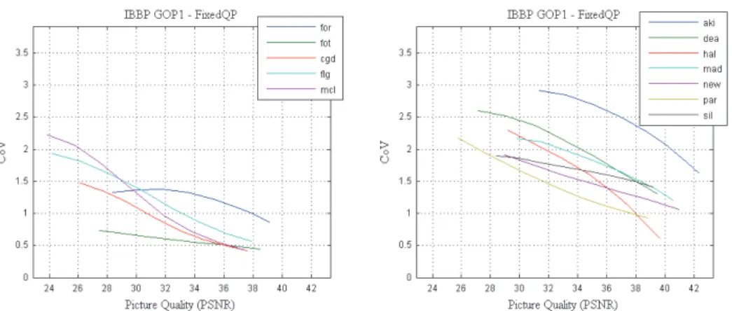
A second important issue for joint video coding broadcasting is the Rate Variability-Distortion (VD). Two sub-sets have been consider from the initial set of twelve video sequences: a first sub-set with camera movement, medium to high spatial detail and temporal complexity (sequences Foreman, Football, Coastguard, Flower Garden, and Mobile and Calendar), and a second sub-set with fixed camera and low to medium spatial detail and motion activity (Akiyo, Deadline, Hall, Mother and Daughter, News, Paris, and Silence). Results are presented in Figure 7, Figure 8, Figure 9, and Figure 10. In the left side it can be observe the results from the first sub-set and in the right the charts for the second sub-set. Simulations results are from open-loop coding setup.
Fig. 7. Rate Variability-distortion (VD) Curve (PSNR; IBBP GOP1).
Fig. 8. Rate Variability-distortion (VD) Curve (PSNR; IBBP GOP2).
Fig. 10. Rate Variability-distortion (VD) Curve (PSNR; IPPP GOP2).
For high spatial complexity and motion activity sequences, variability is significantly lower than the sub-set of sequences with lower spatial and temporal complexity. At the same time, GOP patterns with B frames present higher values of variability regarding GOP patterns without B frames. As frames of type I show lower compression ratio compared to Predicted and Interpolated frames type, the combination of the different types of frames results in the observed higher bit-rate variability.
As the GOP size increases, the amplitude variation regarding the variability increases. This effect is stronger with the video sub-set of lower spatial and temporal complexity sequences. In these cases, motion estimation is very effective resulting in higher compression ratios for P and B pictures comparing to the bits budget of a typical Intra image. B frames, in general, present a small reduction of the variability in sequences with higher complexity. The amplitude of this variation increases while the sequence complexity decreases.
8. Acknowledgment
This work has been supported by “Fundação para a Ciência e Tecnologia” and “Programa Operacional Ciência e Inovação 2010” (POCI 2010), co-funded by the Portuguese Government and European Union by FEDER Program.
9. References
Adjeroh, D.A. & Lee, M.C. (2004). Scene-adaptive transform domain video partitioning,
IEEE Transaction on Multimedia, Vol. 6. No 1 (February 2004), pp 58-69, ISSN
1520-9210.
Bellman, R.E. (2003). Dynamic Programming, Princeton University Press, Dover paperback edition (2003), ISBN 0486428095.
Berger, T. (1971). Rate Distortion Theory, Prentice-Hall, Inc., ISBN 0137531036, Englewood Cliffs, NJ.
Chan, Y.-L & Siu, W.-C. (2001). An efficient search strategy for block motion estimation using image features, IEEE Transactions on Image Processing, Vol 10, No 8 (August 2001), pp 1223-1238, ISSN 1057-7149.
Chen, J.J. & Lin, D.W. (1996). Optimal bit allocation for video coding under multiple constraints, Proceedings of the IEEE International Conference Image Processing 1996, Vol. 3, pp 403 – 406, ISBN 0-7803-3259-8, Lausanne, Switzerland, Sep 16-19, 1996.
Chen, Z. & Ngan, K. N. (2004). Linear rate-distortion models for MPEG-4 shape coding,
IEEE Transactions on Circuits and Systems for Video Technology, Vol. 14, No 6 (June
2004), pp 869–873, ISSN 1051-8215.
Chen, Z. & Ngan, K. N. (2005b). Rate-distortion analysis for MPEG-4 binary shape coding, Proceedings of IEEE International Symposium on Intelligent Signal Processing and Communications Systems, pp 801 - 804, ISBN 0-7803-9266-3, Hong Kong, December 13-16, 2005.
Chen, Z. & Ngan, K. N. (2005a). Joint texture-shape optimization for MPEG-4 multiple video objects, IEEE Transactions on Circuits and Systems for Video Technology, Vol. 15, No 2 (September 2005). pp 1170–1174, ISSN 1051-8215.
Chen, Z. & Ngan, K. N. (2007). Recent advances in rate control for video coding, Signal Processing: Image Communication, Vol 22, No 1 (January 2007), pp 19-38, ISSN 0923-5965.
Chiang, T. & Zhang, Y.-Q. (1997). A new rate control scheme using quadratic rate distortion model, IEEE Transactions on Circuits and Systems for Video Technology, Vol. 7, No 1 (January 1997), pp 246-250, ISSN 1051-8215.
Chung, K.-L. & Chang, L-.C (2003). A new predictive search area approach for fast block motion estimation, IEEE Transactions on Image Processing, Vol. 12, No 6 (June 2003), pp 648-652, ISSN 1057-7149.
Ding, W. & Liu, B. (1996). Rate control of MPEG video coding and recording by rate-quantization modeling, IEEE Transactions on Circuits and Systems for Video
Technology, Vol. 6, No 1 (January 1996), pp 12-20, ISSN 1051-8215.
Everett, H. (1963). Generalized Lagrange multiplier method for solving problems of optimum allocation of resource, in Operations Research, Vol 11, N0. 3, pp 399–417, ISSN 0030-364X.
Forney, G. D. (1973). The Viterbi algorithm, Proceedings of the IEEE , Vol 61, No 3, pp 268–278, ISSN 0018-9219.
Kim, H.M. (2003). Adaptive rate control using nonlinear regression, IEEE Transactions on
Circuits and Systems for Video Technology, Vol. 13, No 5 (May 2003), pp 432-439,
ISSN 1051-8215.
Hang, H. M. & Chen, J.J. (1997). Source model for transform video coder and its application – part I: fundamental theory, IEEE Transactions on Circuits and Systems for Video
Technology, Vol. 7, No 2 (April 1997), pp 287-298, ISSN 1051-8215.
He, Z. & Mitra, S. K. (2002). Optimum bit allocation and accurate rate control for video coding via-domain source modelling, IEEE Transactions on Circuits and Systems for
Video Technology, Vol. 12, No 10 (Octobre 2002), pp 840–849, ISSN 1051-8215.
He, Z. (2001). rho-Domain Rate-Distortion Analysis and Rate Control for Visual Coding and Communication, PhD Dissertation, University of California, Santa Barbara, June 2001.
Huang, J. J. Y. & Schultheiss, P.M. (1963). Block quantization of correlated Gaussian random variables, IEEE Transaction on Communications Systems, Vol 11, N 3, pp 289–296, ISSN 0096-1965.
ISO/IEC (1997). Text of ISO/IEC 14496-2 MPEG-4 Video VM-Version 8.0, ISO/IEC JTC1/SC29/WG11 Coding of Moving Pictures and Associated Audio MPEG 97/W1796, Stochholm, Sweden, July 1997.
ISO/IEC, JTC1/SC29/WG11 (1993). MPEG Video Test Model 5 (TM-5), document MPEG93/457, April 1993.
ITU-T (2005). Rec. H.264.2 : Reference software for advanced video coding, 2005.
ITU-T, SG16 (1997). Video Codec Test Model, near-term, Version 8 (TMN8), Document Q15-A-59, Portland, USA, June 1997.
Kamaci, N.; Altunbasak, Y. & Mersereau, R. M. (2005). Frame bit allocation for the H.264/AVC video coder via Cauchy-density-based rate and distortion models,
IEEE Transactions on Circuits and Systems for Video Technology, Vol. 15, No 5 (August
2005), pp 994–1006, ISSN 1051-8215.
Keesman, G.; Shah, I. & Klein-Gunnewiek, R. (1995). Bit-rate control for MPEG encoders, Signal Processing: Image Communication, Vol 6, No 6 (February 1995), pp 545-560, ISSN 0923-5965.
Lee, H. J.; Chiang, T. & Zhang, Y. Q. (2000). Scalable rate control for MPEG-4 video, IEEE
Transactions on Circuits and Systems for Video Technology, Vol. 10, No 6 (September
2000), pp 878-894, ISSN 1051-8215.
Li, Z. G.; Pan, F.; Lim, K. P.; Feng, G. ; Lin, X. & Rahardja, S. (2003a). Adaptive basic unit layer rate control for JVT, Joint Video Team of ISO/IEC MPEG and ITU-T VCEG, document JVT-G012r1, March 2003.
Li, Z. G.; Gao, W.; Pan, F.; Ma, S. ; Lin, K. P. ; Feng, G.; Lin, X.; Rahardja, S.; Lu, H. & Lu, Y. (2003b). Adaptive Rate Control with HRD Consideration, document JVT-H014, 8th meeting, Geneva, May 2003.
Li, Z. G.; Pan, F.; Lim, K.P.; Feng, G.N. ; Lin, X. ; Rahardja, S. & Wu, D.J. (2003c). Adaptive frame layer rate control for H.264, Proceedings. 2003 International Conference on Multimedia and Expo, 2003, Vol 1, pp 581-584, ISBN 0-7803-7965-9, July 6-9, 2003. Li, Z. G.; Pan, F.; Lim, K.P.; Lin, X. & Rahardja, S. (2004). Adaptive rate control for H.264,
2004 International Conference on Image Processing, pp 745-748, ISBN 0-7803-8554-3, October 24-27, 2004.
Lim, K. P ; Sullivan, G. & Wiegand, T. (2007). Text Description of Joint Model Reference Encoding Methods and Decoding Concealment Methods, Joint Video Team of ISO/IEC MPEG and ITU-T VCEG, document JVT-W057, San Jose, April 2007. Lin, L. J. & Ortega, A. (1998). Bit-rate control using piecewise approximated rate-distortion
characteristics, IEEE Transactions on Circuits and Systems for Video Technology, Vol. 8, No 4 (August 1998), pp 446-459, ISSN 1051-8215.
Lin, L. J.; Ortega, A. & Kuo, C.-C.J.(1996). Rate control using spline-interpolated R-D characteristics, SPIE Visual Communication Image Processing, Cambridge Visual Communication Image Processing, Cambridge, Orlando, FL, 1996, pp. 111-122.
Ma, S.; Gao, W & Lu, Y. (2002). Rate Control on JVT Standard, Joint Video Team (JVT) of ISO/IEC MPEG & ITU-T VCEG (ISO/IEC JTC1/SC29/WG11 and ITU-T SG16 Q.6), document JVT-D030, 4th Meeting: Klagenfurt, Austria, July 22-26, 2002.
Ma, S.; Gao, W. & Lu, Y. (2005). Rate-distortion analysis for H.264/AVC video coding and its application to rate control, IEEE Transactions on Circuits and Systems for Video
Technology, Vol. 15, No 12 (December 2005), pp 1533-1544, ISSN 1051-8215.
Ortega, A. (1996). Optimal bit allocation under multiple rate constraints, Proceedings of the Data Compression Conference, pp 349–358, ISBN 0-8186-7358-3, Snowbird, UT, USA, 31 Mar – 01 April, 1996.
Puri, A.; Hang, H.-M. & Schilling, D. L. (1987). Interframe coding with variable block-size motion compensation, Proceedings of IEEE Global Telecomm. Conf. (GLOBECOM), pp 65-69, 1987.
Ramchandran, K.; Ortega, A. & Vetterli, M. (1993). Bit allocation for dependent quantization with applications to MPEG video codec, 1993 IEEE International Conference on Acoustics, Speech, and Signal Processing, pp. 381-385, ISBN 0-7803-7402-9, Minneapolis, April 27-30, 1993.
Ramchandran, K.; Ortega, A. & Vetterli, M. (1994). Bit allocation for dependent quantization with applications to multiresolution and MPEG video coders, IEEE Transactions on Image Processing, Vol.3, No.5, pp.533-545, ISSN 1057-7149.
Rhee, I.; Martin, G. R. ; Muthukrishnan, S. & Packwood, R. A. (2001). Quadtree-structured variable-size block-matching motion estimation with minimal error, IEEE
Transactions on Circuits and Systems for Video Technology, Vol. 10, No 2 (February
2001), pp 42-50, ISSN 1051-8215.
Ribas-Corbera, J. & Lei, S. (1999). Rate control in DCT video coding for low-delay communications, IEEE Transactions on Circuits and Systems for Video Technology, Vol. 9, No 1 (February 1999), pp 172-185, ISSN 1051-8215.
Ribas-Corbera, J. & Neuhoff, David L. (1998). Optimizing block size in motion compensated video coding, Journal of Electronic Imaging, Vol. 7, No 1 (January 1998), pp.155-165, ISSN 1017-9909.
Ronda, J. I.; Eckert, M.; Jaureguizar, F. & Garcia, N. (1999). Rate control and bit allocation for MPEG-4, IEEE Transactions on Circuits and Systems for Video Technology, Vol. 9, No 12 (December 1999), pp 1243–1258, ISSN 1051-8215.
Schuster, G. M. & Katsaggelos, A.K. (1997a). Rate Distortion based Video Compression, Kluwer Academic Publishers, ISBN 978-1-4419-5172-4, Norwell, MA.
Schuster, G. M. & Katsaggelos, A.K. (1997b). A video compression scheme with optimal bit allocation among segmentation motion and residual error, IEEE Transactions on
Image Processing, Vol 6, No 11 (November 1997), pp 1487–1502, ISSN 1057-7149.
Seeling, P.; Fitzek, F. H. P. & Reisslein, M. (2007). Video Traces for Network Performance Evaluation - A Comprehensive Overview and Guide on Video Traces and Their Utilization in Networking Research, Springer Verlag, 272 pages, ISBN 978-1-4020-5565-2, 2007.
Seeling, P.; Reisslein, M. & Kulapala, B. (2004). Network Performance Evaluation with Frame Size and Quality Traces of Single-Layer and Two-Layer Video: A Tutorial,
IEEE Communications Surveys & Tutorials, Vol. 6, No. 3 (Third Quarter 2004), pp
58-78, ISSN 1553-877X.
Shoham, Y. & Gersho, A. (1988). Efficient bit allocation for an arbitrary set of quantizers,
IEEE Transaction in Acoustics, Speech and Signal Processing, Vol. 36, pages 1445–1453,
ISSN 1053-587X.
Sullivan, G. J. & Wiegand, T. (1998). Rate-distortion optimization for video compression,
IEEE Signal Processing Magazine, Vol. 15, No. 6 (November 1998), pp 74–90, ISSN
1053-5888.
Sullivan, G.J. & Wiegand, T. (1997). A theory for the optimal bit allocation between displacement vector field and displaced frame difference, IEEE Journal on Selected
Areas in Communications, Vol 15, No 9 (December 1997), pp 1739–1751, ISSN
0733-8716.
Tourapis, H.-Y.C. & Tourapis, A.M. (2003). Fast motion estimation within the H.264 codec,
Proceedings. 2003 International Conference on ICME '03, Vol 3, pp 517-520, ISBN
0-7803-7965-9, July 6-9, 2003.
Vardeman, S. (1994). Statistics for Engineering Problem Solving, PWS Publishing Company, ISBN 0-534-92871-4, boston, USA.
Vetro, A. ; Sun, H. & Wang. Y. (1999). MPEG-4 rate control for multiple video objects, IEEE
Transactions on Circuits and Systems for Video Technology, Vol. 9, No 2 (February
1999), pp 186–199, ISSN 1051-8215.
Wiegand, T. & Girod, B. (2001). Lagrange multiplier selection in hybrid video coder control,
Proceedings of 2001 International Conference on Image Processing, pp 542–545, ISBN
0-7803-6725-1, 07 Oct 2001-10 Oct 2001.
Wiegand, T.; Schwarz, H.; Joch, A.; Kossentini, F. & Sullivan, G. J. (2003a). Rate-Constrained Coder Control and Comparison of Video Coding Standards, IEEE Transactions on
Circuits and Systems for Video Technology, Vol. 13, No 7 (July 2003), pp 688-703, ISSN
1051-8215.
Wiegand, T.; Sullivan, G. J. & Luthran, A. (2003b). Draft ITU-T Recommendation H.264 and Final Draft International Standard 14496-10 Advanced Video Coding, Joint Video Team of ISO/IEC JTC1/SC29/WG11 and ITU-T SG16/Q.6, document JVT-G050rl; Geneva, Switzerland, May 2003
Wiegand, T.; Sullivan, G. J.; Bjontegaard, G. & Luthra, A. (2003c). Overview of the H.264/AVC video coding standard, IEEE Transactions on Circuits and Systems for
Video Technology, Vol. 13, No 7 (July 2003), pp 560-576, ISSN 1051-8215.
Wu, Y.; Shouxun, L. & Zhang (2005). Optimum Bit Allocation and Rate Control for H.264/AVC, Joint Video Team (JVT) of ISO/IEC MPEG & ITU-T VCEG (ISO/IEC JTC1/SC29/WG11 and ITU-T SG16 Q.6), document JVT- O016, 15th Meeting, Busan, KR, April 16-22, 2005.
Yan, A. Y. K. & Liou, M. L. (1997). Adaptive predictive rate control algorithm for MPEG videos by rate quantization method, Proceedings on Picture Coding Symposium, pp 619-624, Berlin, Germany, September 1997.
Yin, P. & Boyce, J. (2004). A new rate control scheme for H.264 video coding, Proceedings of ICIP '04. 2004 International Conference on Image Processing, pp 449-452, ISBN 0-7803-8554-3, October 24-27, 2004.
Zhang, J. ; He, Y. ; Yang, S. & Zhong, Y. (2003). Performance and complexity joint optimization for H.264 video coding, Proceedings on IEEE International Symposium
Circuits and Systems 2003 (ISCAS’03), pp 888-891, ISBN 0-7803-7761-3, May 25-28 ,
2003.
Zhang, Z.; Liu, G. ; Li, H. & Li, Y. (2005). A novel PDE-based rate distortion model for rate control, IEEE Transactions on Circuits and Systems for Video Technology, Vol. 15, No (2005), pp 1354–1364, ISSN 1051-8215.