Defective Models for Cure Rate Modeling

(1)

Defective Models for Cure Rate Modeling

(2)

Statistics Department

Ricardo Ferreira da Rocha

Defective Models for Cure Rate Modeling

A thesis submitted to the Statistics

Department at the Federal

University of S˜ao Carlos for the

degree of Doctor in Statistics.

Advisor: Dra_{. Vera Lucia Damasceno Tomazella}

Co-advisors: Dr. Saralees Nadarajah and

Dr. Francisco Louzada-Neto

(3)

R672d

Rocha, Ricardo Ferreira da

Defective models for cure rate modeling / Ricardo Ferreira da Rocha. -- São Carlos : UFSCar, 2016. 139 p.

Tese (Doutorado) -- Universidade Federal de São Carlos, 2016.

(4)

(5)

Modeling of a cure fraction, also known as long-term survivors, is a part of survival

analysis. It studies cases where supposedly there are observations not susceptible to the

event of interest. Such cases require special theoretical treatment, in a way that the

modeling assumes the existence of such observations. We need to use some strategy to

make the survival function converge to a valuep_∈(0,1), representing the cure rate. A way

to model cure rates is to use defective distributions. These distributions are characterized

by having probability density functions which integrate to values less than one when the

domain of some of their parameters is different from that usually defined. There is not

so much literature about these distributions. There are at least two distributions in the

literature that can be used for defective modeling: the Gompertz and inverse Gaussian

distribution. The defective models have the advantage of not need the assumption of the

presence of immune individuals in the data set. In order to use the defective distributions

theory in a competitive way, we need a larger variety of these distributions. Therefore, the

main objective of this work is to increase the number of defective distributions that can be

used in the cure rate modeling. We investigate how to extend baseline models using some

family of distributions. In addition, we derive a property of the Marshall-Olkin family of

distributions that allows one to generate new defective models.

Keywords: Cure fraction, Defective models, Inverse Gaussian distribution, Gompertz distribution, Kumaraswamy family, Long-term survivors, Marshall-Olkin family, Survival

analysis.

(6)

A modelagem da fra¸cão de cura é uma parte importante da análise de sobrevivência.

Essa área estuda os casos em que, supostamente, existem observa¸cões não suscept´ıveis

ao evento de interesse. Tais casos requerem um tratamento te´orico especial, de forma

que a modelagem pressuponha a existência de tais observa¸cões. É necessário usar alguma

estratégia para tornar a fun¸cão de sobrevivência convergente para um valorp_∈(0,1), que

represente a taxa de cura. Uma forma de modelar tais fra¸cões é por meio de distribui¸cões

defeituosas. Essas distribui¸cões são caracterizadas por possu´ırem fun¸cões de densidade

de probabilidade que integram em valores inferiores a um quando o dom´ınio de alguns

dos seus parâmetros é diferente daquele em que é usualmente definido. Existem, pelo

menos, duas distribui¸c˜oes defeituosas na literatura: a Gompertz e a inversa Gaussiana.

Os modelos defeituosos tˆem a vantagem de n˜ao precisar pressupor a presen¸ca de indiv´ıduos

imunes no conjunto de dados. Para utilizar a teoria de distribui¸c˜oes defeituosas de forma

competitiva é necessário uma maior variedade dessas distribui¸cões. Portanto, o principal

objetivo deste trabalho é aumentar o número de distribui¸cões defeituosas que podem ser

utilizadas na modelagem de fra¸c˜oes de curas. N´os investigamos como estender os modelos

defeituosos básicos utilizando certas fam´ılias de distribui¸cões. Além disso, derivamos uma

propriedade da fam´ılia Marshall-Olkin de distribui¸c˜oes que permite gerar uma nova classe

de modelos defeituosos.

Palavras-Chave: Análise de sobrevivência, Distribui¸cão inversa Gaussiana, Distribui¸cão Gompertz, Fam´ılia Kumaraswamy, Fam´ılia Marshall-Olkin, Fra¸cão de cura, Modelos de

longa dura¸c˜ao, Modelos defeituosos.

(7)

List of Figures ix

List of Tables xi

1 Preliminaries 1

1.1 Introduction . . . 1

1.2 Theoretical Background . . . 3

1.2.1 Survival Analysis . . . 3

1.2.2 Kaplan-Meier Estimator . . . 6

1.2.3 Cure Rate Models. . . 7

1.2.4 Maximum Likelihood Estimation . . . 9

1.3 Artificial Data Generation Algorithm . . . 12

1.4 Data Sets . . . 13

1.4.1 Leukemia . . . 13

1.4.2 Melanoma . . . 14

1.4.3 Colon . . . 15

1.4.4 Divorce . . . 15

1.4.5 Second Birth . . . 16

1.5 Objectives and Overview . . . 18

2 Defective Cure Rate Models 19 2.1 Introduction . . . 19

2.2 Methodology . . . 19

2.2.1 Defective Models . . . 19

2.2.2 The Defective Gompertz Distribution . . . 21

2.2.3 The Defective Inverse Gaussian Distribution . . . 22

2.2.4 Inference . . . 23

2.3 Simulation Studies . . . 25

2.4 Applications . . . 27

2.4.1 Leukemia data . . . 28

2.4.2 Melanoma data . . . 29

2.4.3 Second Birth data . . . 31

2.4.4 Divorce data . . . 31

(8)

2.5 Conclusions . . . 33

3 Marshall-Olkin Family of Defective Models 35 3.1 Introduction . . . 35

3.2.1 The Marshall-Olkin Gompertz distribution . . . 37

3.2.2 The Marshall-Olkin inverse Gaussian distribution . . . 38

3.2.3 Inference . . . 39

4 Kumaraswamy Family of Defective Models 54 4.1 Introduction . . . 54

4.2.1 The Kumaraswamy family of distributions . . . 55

4.2.2 The Kumaraswamy Gompertz distribution . . . 58

4.2.3 The Kumaraswamy inverse Gaussian distribution . . . 59

4.2.4 Inference . . . 60

4.2.5 The Kumaraswamy-G regression model . . . 61

4.4.2 Colon data . . . 68

4.4.4 Discussion . . . 71

5 Generalized Extended Class of Defective Models 74 5.1 Introduction . . . 74

5.2 Distribution Families . . . 75

5.2.1 Gamma G . . . 76

5.2.2 Gamma Uniform G . . . 77

5.2.3 Exponentiated G . . . 78

5.2.4 Truncated-Exponential Skew-Symmetric G . . . 79

5.2.5 Beta G . . . 79

5.2.6 Exponentiated Exponential Poisson G . . . 82

5.2.7 Exponentiated Generalized G . . . 82

5.2.8 Weibull-G . . . 83

(9)

6 A Special Class of Defective Models Based on the Marshall-Olkin Family 96 6.1 Introduction . . . 96

6.2.1 The Marshall Olkin family . . . 97

6.2.2 The extended Weibull distribution . . . 99

6.2.3 Inference . . . 102

6.2.4 Defective Marshall Olkin-G regression model . . . 103

6.3 Simulation studies . . . 104

6.4 Real data applications . . . 109

6.4.2 Colon data . . . 111

6.4.3 Divorce data . . . 113

6.4.5 Discussion . . . 116

7 Final Remarks 119 7.1 Conclusions . . . 119

7.2 Future Works . . . 121

7.3 Acknowledgements . . . 122

(10)

1.1 Kaplan-Meier and estimated cumulative hazard curves for the leukemia

data set. . . 14

1.2 Kaplan-Meier and estimated cumulative hazard curves for the melanoma

data set. . . 15

1.3 Kaplan-Meier and estimated cumulative hazard curves for the colon data

set. . . 16

1.4 Kaplan-Meier and estimated cumulative hazard curves for the divorce data

set. . . 17

1.5 Kaplan-Meier and estimated cumulative hazard curves for the birth data set. 17

2.1 Example of a cumulative function of a defective distribution. . . 20

2.2 Density, survival and hazard functions of the defective Gompertz distribution. 22

2.3 Density, survival and hazard functions of the defective inverse Gaussian

distribution. . . 23

2.4 Mean squared errors, biases and coverage probabilities of _ba,bb,_bp

ver-sus n for simulated data from the Gompertz distribution with (a, b, p) =

(₋1,1,0.3678). . . 25

2.5 Mean squared errors, biases and coverage probabilities of _ba,bb,_bp

ver-sus n for simulated data from the Gompertz distribution with (a, b, p) =

(−2,1,0.6065). . . 26

2.6 Mean squared errors, biases and coverage probabilities of _ba,bb,p_bversus n

for simulated data from the inverse Gaussian distribution with (a, b, p) =

(₋1,5,0.3296). . . 27

2.7 Mean squared errors, biases and coverage probabilities of _ba,bb,p_bversus n

for simulated data from the inverse Gaussian distribution with (a, b, p) =

(₋1,1,0.8646). . . 28

2.8 Fitted survival curves of the Gompertz and inverse Gaussian distributions

in the leukemia data set. . . 29

(11)

in the melanoma data set. . . 30

in the second birth data set . . . 32

in the divorce data set . . . 33

3.1 Density, survival and hazard functions of the defective Marshall-Olkin

Gompertz distribution. . . 38

3.2 Density, survival and hazard functions of the defective Marshall-Olkin

in-verse Gaussian distribution. . . 39

3.3 Mean squared errors, biases, coverage probabilities and coverage lengths of

b

a,bb,r,_b p_b versus n for simulated data from the Marshall-Olkin Gompertz

distribution with (a, b, r, p) = (₋3,4,2,0.4172). . . 42

3.4 Mean squared errors, biases, coverage probabilities and coverage lengths

of _ba,bb,_br,p_b versus n for simulated data from the Marshall-Olkin inverse

Gaussian distribution with (a, b, r, p) = (₋2,10,2,0.4958).. . . 43

3.5 In the left, the plotted line represents the difference between the AIC values

obtained under the Marshall-Olkin Gompertz mixture and defective mod-els, respectively, when the data were generated from a defective model. In

the right, the corresponding estimates of p. . . 44

obtained under the Marshall-Olkin inverse Gaussian mixture and defective models, respectively, when the data were generated from a defective model.

In the right, the corresponding estimates of p. . . 44

3.7 In the left, the plotted line represents the difference between the AIC

val-ues obtained under the Marshall-Olkin Gompertz mixture and defective models, respectively, when the data were generated from a mixture model.

obtained under the Marshall-Olkin inverse Gaussian mixture and defective models, respectively, when the data were generated from a mixture model.

3.9 Survival curves for the fitted Gompertz, Marshall-Olkin Gompertz,

in-verse Gaussian and Marshall-Olkin inin-verse Gaussian distributions for the

leukemia data set. . . 48

3.10 Survival curves for the fitted Gompertz, Marshall-Olkin Gompertz, inverse Gaussian and Marshall-Olkin inverse Gaussian distributions for the second

(12)

3.11 Survival curves for the fitted Gompertz, Marshall-Olkin Gompertz, inverse Gaussian and Marshall-Olkin inverse Gaussian distributions for the colon

data set. . . 49

3.12 Plots of the Kaplan-Meier estimates of the survival function versus the predicted values from the proposed distributions. The top four plots are for the second birth data set. The middle four plots are for the leukemia

data set. The bottom four plots are for the colon data set. . . 50

4.1 Probability density, survival and hazard functions of the defective

Ku-maraswamy Gompertz distribution. . . 58

4.2 Probability density, survival and hazard functions of the defective

Ku-maraswamy inverse Gaussian distribution. . . 59

4.3 Survival curves for the fitted distributions for the melanoma data set. . . . 65

4.4 In the left, the fitted Gompertz regression model, in the right, the inverse

Gaussian model. . . 67

4.5 In the left, the fitted Kumaraswamy Gompertz regression model, in the

right, the Kumaraswamy inverse Gaussian model. . . 67

4.6 Survival curves for the fitted distributions for the colon data set. . . 68

4.7 Survival curves for the fitted distributions for the leukemia data set. . . 70

4.8 Probability plots for the fit of the four distributions to the three data sets. 71

the estimators of a, b, r and p versus n for the Exponentiated Gompertz

of the estimators of a, b, r and p versus n for the TESS inverse Gaussian

of the estimators of a, b, r, u and p versus n for the Weibull Gompertz

distribution with (a, b, r, u, p) = (−1,2,2,2,0.3678). . . 87

the estimators of a, b, r, u and p versus n for the EEP inverse Gaussian

distribution with (a, b, r, u, p) = (−1,2,1,2,0.3976). . . 88

5.5 Fitted survival curves of the proposed models when the baseline

distribu-tion is Gompertz, in the leukemia data set. . . 90

distribu-tion is inverse Gaussian, in the leukemia data set. . . 91

(13)

distribu-tion is inverse Gaussian, in the melanoma data set. . . 94

6.1 From the left to the right, from the top to the bottom, the density and sur-vival functions of the proposed distributions, in the same order presented in Table 6.1. The parameter values used areu= (₋0.2,₋0.5,₋1,₋0.2,₋0.5,₋1), v = (−0.5,−0.5,−0.5,−2,−2,−2),a= (0.5,0.5,1,1,2,2),b= (1,1,2,2,0.5,0.5) and c = (2,2,0.5,0.5,1,1). The colors are (black, red, green, blue, light blue, pink). . . 100

6.2 Mean squared errors, biases, coverage probabilities and coverage lengths of the estimators of r, v and p versus n for the Marshall Olkin-Lomax distribution with (r, v) = (₋1,₋10). . . 104

6.3 Mean squared errors, biases, coverage probabilities and coverage lengths of the estimators of r, v, a and p versus n for the Marshall Olkin-Weibull distribution with (r, v, a) = (−1,−2,3). . . 105

6.4 Mean squared errors, biases, coverage probabilities and coverage lengths of the estimators of r, v, a and p versus n for the Marshall Olkin-Chen distribution with (r, v, a) = (₋1,₋2,2). . . 106

6.5 Mean squared errors, biases, coverage probabilities and coverage lengths of the estimators of r, v, a and p versus n for the Marshall Olkin-Burr XII distribution with (r, v, a) = (₋1,₋2,2). . . 107

6.6 Fitted distributions for the leukemia data set. . . 110

6.7 Fitted distributions for the colon data set. . . 112

6.8 Fitted distributions for the divorce data set. . . 114

(14)

2.1 Maximum likelihood estimates of the Gompertz and inverse Gaussian

dis-tributions in the leukemia data set. . . 28

dis-tributions in the melanoma data set . . . 30

dis-tributions in the second birth data set . . . 31

dis-tributions in the divorce data set . . . 31

3.1 MLEs for the fits of the Gompertz and Marshall-Olkin Gompertz

distribu-tions for the leukemia data set. . . 51

distribu-tions for the second birth data set. . . 51

distribu-tions for the colon data set. . . 52

3.4 MLEs for the fit of the Marshall-Olkin inverse Gaussian distribution for

the leukemia data set. . . 52

the second birth data set. . . 53

the colon data set. . . 53

3.7 AIC values for the fitted defective distributions compared with their

re-spective mixture models. . . 53

4.1 Simulation of the maximum likelihood estimates for mean and standard

deviation of the Kumaraswamy Gompertz distribution. . . 62

4.2 Simulation of the maximum likelihood estimates for mean and standard

deviation of the Kumaraswamy inverse Gaussian distribution. . . 63

4.3 MLEs for the fitted distributions for the melanoma data set. . . 65

(15)

4.4 MLEs for the fitted regression models for the melanoma data set. . . 66

4.5 MLEs for the fitted distributions for the colon data set. . . 68

4.6 MLEs for the fitted distributions for the leukemia data set. . . 69

4.7 Log-likelihood ratio test for the proposed models and data sets. . . 72

4.8 95 percent asymptotic confidence intervals for the parameter afor the pro-posed models and data sets. . . 72

4.9 AIC values for the fitted distributions and for the standard mixture model. The smaller AIC values are bolded. . . 72

5.1 Maximum likelihood estimates in the leukemia data set of the proposed models when the baseline distribution is Gompertz. . . 89

5.2 Maximum likelihood estimates in the leukemia data set of the proposed models when the baseline distribution is inverse Gaussian. . . 89

5.3 Maximum likelihood estimates in the melanoma data set of the proposed models when the baseline distribution is the Gompertz . . . 92

5.4 Maximum likelihood estimates in the melanoma data set of the proposed models when the baseline distribution is the inverse Gaussian. . . 92

6.1 Some particular cases of the extended Weibull distribution. . . 99

6.2 MLEs for the fitted distributions and some measures for the leukemia data set. . . 111

6.3 MLEs for the fitted distributions and some measures for the colon data set. 111 6.4 MLEs for the fitted distributions and some measures for the divorce data set. . . 113

6.5 MLEs for the fitted regression models and the AIC measure for the melanoma data set. . . 115

6.6 Comparison of the AIC value of the mixture and defective models. . . 117

(16)

Preliminaries

1.1 Introduction

Modeling of a cure fraction, also known as long-term survivors, is a part of survival

analysis. It studies cases where supposedly there are observations not susceptible to the

event of interest. Such cases require special theoretical treatment, in a way that the

modeling assumes the existence of such observations. In the standard theory of survival

analysis the survival function S(t) tends to zero as time increases. We need to use some

strategy to make the survival function converge to a value p _∈ (0,1), representing the

cure rate.

The method most commonly used is the standard mixture model, initially proposed by

Boag(1949) andBerkson & Gage(1952). The model is described byS(t) = p+(1−p)S0(t),

where S0(t) is a proper survival function. Common choices for S0(t) are the Weibull,

Gompertz and lognormal distributions, according to Ibrahim et al. (2005). Tsodikov

et al.(2003) proposed a non-mixture model defined in terms of a cumulative hazard rate

function. Its survival function has the formS(t) = pF0(t), where F

0(t) represents a proper

distribution function. More about this method can be found in Martinez et al. (2013).

Many other methods are known for cure rate modeling, see, for example, Cooner et al.

(2007),Rodrigueset al.(2009a),Nieto-Barajas & Yin(2008) and the bookMaller & Zhou

(1996).

(17)

The literature regarding to cure rate models are very large and have lots of different

approaches on how estimate the quantities of interest. In Chen et al. (1999) is

pro-posed some Bayesian models to estimate cure fractions. In Sy & Taylor (2000) is

dis-cussed maximum likelihood techniques in an Cox proportional hazards structure of cure

model. In Rodrigues et al. (2009b), its used the Conway-Maxwell Poisson as the

distri-bution of competing causes, as proposed in Rodrigues et al. (2009a). In Yin & Ibrahim

(2005) an unified approach is presented based in the Box-Cox transformation. In Peng

& Xu (2012) an extension of the model presented in Yin & Ibrahim (2005) are done and

some model selection criteria are discussed. In Balakrishnan & Pal (2012) is proposed

an expectation-maximization algorithm to do estimation in the model proposed in

Ro-drigues et al. (2009b), where the time-to-event is assumed exponential. In Balakrishnan

& Pal(2013a), Balakrishnan & Pal (2013b) and Balakrishnan & Pal (2015), the authors

keeps developing the EM algorithm but with Weibull, lognormal and generalized gamma

distributions to the time-to-event.

Another way to model cure rates is to use defective distributions, as explored in this thesis.

Defective distributions are characterized by having probability density functions which

integrate to values less than 1 when the domain of some of their parameters is different

from that usually defined. There is not so much literature about these distributions. There

are at least two distributions in the literature that can be used for defective modeling:

the Gompertz and inverse Gaussian distributions. The use of these defective distributions

became more appealing after the works of Balka et al. (2009) and Balka et al. (2011),

although some previous papers have used the same idea. In Whitmore (1979), the term

defective was used to refer to the inverse Gaussian distribution that allows one of its

parameters to be negative.

The Gompertz distribution becomes defective when its shape parameter is negative. It

first appeared in Haybittle (1959), where it was used to model a breast cancer data set.

Cantor & Shuster (1992) applied a modified version of this distribution to a pediatric

cancer data set. Gieser et al. (1998) extended the distribution to include covariates.

More recently,Rochaet al. (2014) performed Bayesian estimation of this distribution. In

(18)

In that work, the authors called the gompertz distributions that allows the parameters

outside their usual domain ofnegative Gompertz.

The inverse Gaussian distribution was first proposed inSchr¨odinger(1915) for calculating

the first time passage probability of a one-dimensional Brownian motion (Wiener process).

More details were studied in Tweedie (1945) and Whitmore (1979). Defective versions

were investigated inBalkaet al.(2009) andBalkaet al.(2011), with classical and Bayesian

approaches. Having only two distributions is not enough to provide sufficient flexibility.

So, the main goal of this thesis is to provide more distributions with the defective property.

In the next section we present all the basic theoretical components needed to understand

and interpret the results in the next chapters. Further, we also present the algorithm to

generate artificial data and five real data sets that are used in some chapters of this thesis.

In the end, we discuss the objectives and a general overview of this work.

1.2 Theoretical Background

Here we show the first definitions in the survival analysis area, since its basic relations

until the unified theory for cure modeling, and it estimation by maximum likelihood.

1.2.1 Survival Analysis

Survival analysis, or reliability analysis, is the branch of statistics that study data normally

associated to the duration of time until the occurrence of an event of interest. The time

can be from the duration of an electronic component or the lifetime of patients with serious

diseases. It does not have to be necessarily an time to event kind of data. For example, we

can check how many kilometers can a tire work properly without replacement. The main

areas of interest are: medicine, biology, engineering, statistics, economics, social sciences,

among others.

What makes the survival analysis a particular area is their specific characteristic to take

(19)

presence of censoring, it is impossible to apply standard statistical for analyzing such

data. There are some kinds of censoring, described in the following.

According to Colosimo & Giolo (2006), the type I censorship or right-censorship, occurs

when the time to the end of the study is pre-established. Thus, some individuals fail

to experience the event of interest in the end of this study, and their lifetimes are right

censored. An example of this type of censorship is when a bank want to check the

time until the customers of a particular portfolio become a bad payer. It is studied

this portfolio for a predetermined amount of time by the institution and at end, some

elements will not experience the event of interest (and therefore are not considered bad

payers). This censoring also occurs when, for some reason, the subject in study is not

available anymore. That could be, for example, someone that quits a drug trial for lack

of motivation, or because the event of interest cannot be observed after some point.

The type II censorship occurs when the study is finished after a certain number n of

individuals experience the event of interest, that is, after a numbernof the research trials

is completed and the individuals who have left to experience the event of interest will be

considered censored.

The random censorship, unlike the others, is a kind of censorship that is beyond the control

of the researcher. It usually occurs when a person leave a given experiment without having

experienced the event of interest. The random censorship is a more common case, with

the particular case censorship Type I, for example, if the patient die for a different reason

of the one considered in the study.

In this work, we represent the data and the censoring by the following: each subject is

observed and denoted by (ti,δi), in which ti is the time until the fail or censoring and δi

is the variable that indicates if that observation was as fail or a censoring. Ifδi = 1, then

the fail was observed. Ifδi = 0, a censoring occurred.

Suppose now that the random variable T,T _≥0, have density function denoted by f(t).

(20)

probability of a subject fails in the interval of time [t, t+ ∆t]:

f(t) = lim

∆t−→0

P(t_≤T < t+ ∆t)

∆t .

Its cumulative function is given by:

F(t) =P(T ≤t) =

Z t

0

f(u)du.

To estimate the probability of an individual survive at least until the timet is one of the

major interests of the survival analysis. So, it is defined the survival function, given by:

S(t) =P(T > t) =

Z ∞

t

f(u)du= 1−F(t).

Of course, the properties of this function are quite similar to the cumulative function:

S(t) is not increasing;S(0) = 1 and limt→∞S(t) = 0.

Other function of huge importance is the hazard function, also called hazard rate function,

that provides the instant rate of fail, that is, knowing that a subject survived until the

timet, this function represents the chance of this subject will fail in the timet+ ∆t, with

∆t _→0. The hazard function is defined by:

h(t) = lim

∆t→0

P(t_≤T < t+ ∆t_|T _≥t)

∆t .

Graphically, the hazard function can have several forms. The cases most studied is where

the hazard function is increasing, decreasing, constant, unimodal and bathtub shaped.

Checking the hazard behavior is important when someone have to choose between

para-metric models. The cumulative hazard function is defined by:

H(t) =

Z t

0

h(u)du. (1.1)

(21)

between them are:

h(t) = f(t)

S(t) =−

d

dtlog[S(t)],

H(t) = ₋log[S(t)],

S(t) = exp[₋H(t)].

1.2.2 Kaplan-Meier Estimator

In the survival analysis literature can be found some estimators of a survival function

obtained through non-parametric techniques. We can refer, for instance, the Nelson-Aalen

estimator, proposed by Nelson (1972) and then reviewed by Aalen (1978), and the one

proposed byKaplan & Meier(1958). This last one is the most important non-parametric

estimator and is described next. For that, consider the following:

• t(1) < t(2) < . . . < t(k), j = 1, . . . , k, the k ordered distinct fail times;

• dj the number of fails in t(j), j = 1, . . . , k;

• nj the number of individuals at risk in t(j), that is, the individuals that not failed

or got censored until the moment instantly previous to t(j).

This way, Kaplan-Meier (KM) estimator is defined by:

b

S(t) = Y

j:tj<t

nj −dj

nj

= Y

j:tj<t

1− dj

nj

.

This expression leads to a ladder function with steps in the observed fail times. In

the paper where it is proposed, the authors justify the expression by showing that this

estimator is the maximum likelihood estimation for S(t). Because of this, one of the

most usual ways to check the fit of an proposed parametric model is to compare it to the

Kaplan-Meier curve. The better the KM captures the fitted model, the better the model

(22)

1.2.3 Cure Rate Models

The survival theory has been widely explored by many researchers in various areas, with a

major focus on analysis of clinical data. Generally the survival functionS(t) = P(T > t)

is the function used to represent the random behavior of T. A property of S(t) is that

it goes to zero as the time pass, which characterizes an event of interest that eventually

always occur.

However, there are situations in which a portion of the population is considered cured

and cannot fail. For example, there are cases when it is considered the recurrence of

a cancer. Some people can have the recurrence, however, there may be some others

that is completely cured from that cancer and, therefore, it would never recur. To solve

such problems,Berkson & Gage (1952), based on the work of Boag(1949), proposed the

standard mixture model for cured fraction. The survival function is set to

S(t) =p+ (1−p)S0(t),

in a way thatS0(t) is a proper survival function. Thus, it follows that S(t) converges to

p as the time increases. In Berkson & Gage (1952) is made an analysis in patients with

stomach cancer, and from there, several other studies of cure rate have been proposed

in the literature, focusing on that model standard mixture. The most common choices

common to S0(t) are the Weibull, log-logistic and log-normal distributions. Recently,

different models have been proposed for this purpose, as inYakovlev & Tsodikov(1996),

Chenet al. (1999) and Ibrahim et al. (2005).

In addition to this approach, we have a unified long-term theory, proposed byRodrigues

et al. (2009a) that generalizes, among others, the mixture model. Let N be a random

variable that represents the number of causes of risk, for a particular event of interest,

with probability distribution of

pn=P[N =n],

(23)

v = 1, . . . , n, be independent, non-negative random variables, with distribution function

F(t) = 1₋S(t). Consider also thatN is independent ofZv, where Zv represents the time

until the occurrence of an particular event of interest, because of thev-th cause of risk.

The time of occurrence of the event of interest is defined as:

T = min_{Z1, Z2. . . , ZN}, (1.2)

in which P[Z0 =_∞] = 1, leads to a proportion p0 of the non-susceptible subjects to the

event of interest. The variablesZv are latent and T is an observable random variable or

censoring. The survival function of the random variableT is given by: Spop(t) = P[T > t].

Let_{an}be a sequence of real numbers and s∈[0,1]. Consider then the following:

A(s) = a0+a1s+a2s2+· · · .

According toFeller (1968), ifA(s) converges, thenA(s) ´e defined as the generating

func-tion of the sequence_{an}. Given a proper survival function S(t), the survival function of

the random variableT, as in (1.2), is given by

Spop(t) = A[S(t)] =

∞

X

n=0

pn[S(t)]n. (1.3)

The proof is in Rodrigues et al. (2009a). This implies that lim

t→∞Spop = P[N = 0] = p0,

with p0 denoting the cured fraction.

The survival function Spop(t) obtained in (1.3) is not proper. The associated density and

hazard function are given, respectively, by:

fpop(t) = f(t)

d

dsA[S(t)],

hpop(t) =

fpop(t)

Spop(t)

= f(t)

Spop(t)

d

dsA[S(t)].

Some examples of generating function can be obtained by using the distributions: Bernoulli,

(24)

the distribution for N is Bernoulli, then Spop is the same proposed in Berkson & Gage

(1952). In Feller (1968) we can check that the generating function for the Bernoulli(θ)

distribution is A(u) =θ+ (1₋θ)u. Thus, we have the mixture model

Spop(t) = A[S(t)] =θ+ (1−θ)S(t).

If we assume the distribution for N is Poisson, then Spop is the same proposed in Chen

et al.(1999), the promotion time cure model.

1.2.4 Maximum Likelihood Estimation

In survival analysis, one of the concerns is to fit parametric models to the observed data,

because they have a more natural interpretation and can calculate the needed probabilities

more adequately.

Based on results obtained from samples, the maximum likelihood estimator selects the

best set of parameters for the alleged distribution of the data. The maximum likelihood

method is able to incorporate censorship and has excellent properties for large samples

(asymptotic results), and is, therefore, the most widely used method for survival analysis.

As censored data bring us important information, we cannot leave it aside. Its contribution

to L(θ) is given by the survival function S(t). Thus, the observations of the random

sample can be divided into two sets, the censored and uncensored.

Suppose that the data are independently and identically distributed and come from a

dis-tribution with density and survival functions specified byf(_·,θ) andS(_·,θ), respectively,

where θ = (θ1, . . . , θk)′ denotes a vector of parameters. Consider a data set D = (t,δ),

wheret= (t1, . . . , tn)′ are the observed failure times andδ = (δ1, . . . , δn)′ are the censored

failure times. The δi is equal to 1 if a failure is observed and 0 otherwise.

The likelihood function ofθ can be written as (see Klein & Moeschberger (2003))

L(θ;D)∝

n

Y

i=1

h

f(ti;θ)δiS(ti;θ)1−δi

i

(25)

The corresponding log-likelihood function is

logL(θ,D) = const +

n

X

i=1

δilogf(ti,θ) +

n

X

i=1

(1₋δi) logS(ti,θ).

This expression is valid for censoring type I, type II, random and when the censor

mech-anism is not informative. The maximum likelihood estimator is the value ofθ that

maxi-mizesL(θ), or, equivalently, its log-likelihood function,l(θ) = log(L(θ)). The estimators

are found by solving the system of equations

U(θ) = ∂ℓ(θ)

∂θj

= 0,

forj = 1, ...k.

Normally, the maximum likelihood estimator does not have a closed expression. That is

due to the complexity that the equations can get depending on the assumed parametric

model for the data in question. So, usually it is necessary to use computational methods

to calculate the maximum likelihood estimates numerically. There are various routines

available for numerical maximization. We used the routine optim in the R software (R

Core Team,2013). The maximization algorithm used was theBFGS, for more information

on this method, please seeLiu & Nocedal(1989). All estimation procedures by maximum

likelihoods done in this thesis was done in R, using optim with BFGS.

Confidence intervals for the parameters were based on asymptotic normality. Ifθbdenotes

the maximum likelihood estimator ofθthen it is well known that the distribution ofθb₋θ

can be approximated by a k-variate normal distribution (where k denotes the length of

(26)

denotes the observed information matrix defined by

I(θ) = ₋            

∂2logL

∂θ₁2

∂2logL

∂θ1∂θ2 · · ·

∂2logL

∂θ1∂θk

∂2logL

∂θ2∂θ1

∂2logL

∂θ2₂ · · ·

∂2logL

∂θ2∂θk

... ... . .. ...

∂2logL

∂θk∂θ1

∂2logL

∂θk∂θ2 · · ·

∂2logL

∂θ2_k

           

.

So, an approximate 100(1 ₋ α) percent confidence interval for θi is

b

θi −zα/2

√

Iii_,_θb

i+zα/2

√

Iii_{, where} _Iii _{denotes the} _i_{th diagonal element of the inverse}

of I and za denotes the 100(1−a) percentile of a standard normal random variable.

In the defective distributions theory, the cured fractionpis calculated as a function of the

estimated parameters. To estimate the variance ofpis used the delta method with a first

order Taylor’s approximation. For more on the delta method, please seeOehlert(1992).

We will also consider some measures to check the relative quality of a fitted model: the

AIC (Akaike Information Criterion), BIC (Bayesian Information Criterion) and CAIC

(Consisten Akaike Information Criterion). They are not a measure of quality by itself,

but is useful to compare between fitted models. Therefore, these measures provides a way

of model selection. The definitions are:

AIC = 2k−2 log(L),

BIC = klog(n)₋2 log(L),

CAIC = k[log(n) + 1]₋2 log(L),

where k is the number of parameters in the model, n is the sample size and L is the

likelihood value in the estimated parameters. The better fit is the one with the lowest

(27)

1.3 Artificial Data Generation Algorithm

Here we describe the data generation used in order to assess the performance of the

maximum likelihood estimates with respect to sample size and to show, among other

things, that the usual asymptotes of maximum likelihood estimators still hold for defective

distributions. The assessment is based on simulations. In all chapters, the simulation

studies are based in this setup. The description of the data generation is given below.

Suppose that the time of occurrence of an event of interest has cumulative distribution

function F(t). We want to simulate a random sample of size n containing real times,

censored times and a cure fraction ofp. An algorithm for this purpose is:

• Determine the desired parameter values, as well as the value of the cure fraction p;

• Generate Mi ∼ Bernoulli(1−p);

• If Mi = 0 set t′i = ∞. If Mi = 1 take t′i as the root of F(t) = u, where u ∼

uniform(0,1−p);

• Generate u′

i ∼ uniform(0,max (ti)), considering only the finite ti;

• Calculate ti = min (t′i, u′i). If ti < u′i setδi = 1, otherwise set δi = 0.

Note that the range of F(t) has been changed and some adjustments made. Instead of

(0,1), we have used (0,1₋p). Therefore, in the third step of the algorithm, the root

of F(t)−u = 0 must be for u ∼ uniform(0,1−p). In the fourth step, the censoring

distribution chosen is a uniform(0,max (ti)). The limit max (ti) was taken in order to

control the censoring regardless of the initial parameter choices. In this way, the censoring

rates were kept reasonable, as described above.

In the simulations, we always have to choose the values of the parameters in the

distri-bution that we want to analyze. Also, we always choose the value ofS = 1000 simulation

per sample size. In each sample size, we calculate the bias, mean square error, coverage

(28)

The following equations were used:

Var(θb) = 1

S S

X

i=1

b

θi −θ

2

,

Bias(θb) = θb₋θ,

MSE(bθ) = Var(bθ) + Bias2(bθ).

The coverage probability is the frequency in which the real parameter value stays in the

confidence region, for each simulation. According to Calsavara (2011), if we consider the

S simulations results done as a result of a binomial experiment with parameter 0.95 (the

significance level), a test to check proportions equivalence can be performed. This way, we

haven1 and n2 such thatP(n1 _≤p_≤n2) = 0.95. That is, given a number of simulations

S, we can expect that the coverage probability will stay betweenn1 and n2 about 95% of

the time. When S = 1000, we have n1 = 0.936 and n2 = 0.964. The coverage length is

the difference between the upper and lower confidence bounds.

1.4 Data Sets

Here we described the five data sets used in the following chapters. They were chosen to

represent a variety of sample sizes, survival and hazard curves. Three of them is of the

clinical area and the other two are related to social sciences studies.

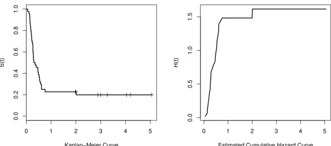
1.4.1 Leukemia

This data set relates to a study of recurrence of leukemia in patients who were submitted

to a certain kind of transplantation. Leukemia is a type of cancer that affects the white

blood cells produced by the bone marrow and can take several forms. The data set

has forty four observations with 20.45 percent censoring (nine in total). The maximum

observation time was approximately five years. For details of this data set, see Kersey

et al.(1987). Figure1.1 shows the Kaplan-Meier and the cumulative hazard curves. The

(29)

0 1 2 3 4 5

0.0

0.2

0.4

0.6

0.8

1.0

Kaplan−Meier Curve

S(t)

0 1 2 3 4 5

0.0

0.5

1.0

1.5

Estimated Cumulative Hazard Curve

H(t)

Figure 1.1: Kaplan-Meier and estimated cumulative hazard curves for the leukemia data set.

1.4.2 Melanoma

This data set collected in the period 1991-1998 is related to a clinical study in which

patients were observed for recurrence after a removal of a malignant melanoma. Melanoma

is a type of cancer that develops in melanocytes, responsible for skin pigmentation. It is a

potentially serious malignant tumor that may arise in the skin, mucous membranes, eyes

and central nervous system, with a great risk of producing metastases and high mortality

rates in the later stages. There are 417 observed times, of which 232 were censored (55.63

percent). For details of this data, seeIbrahim et al. (2001).

This data set has covariates information, which is used to illustrate regression models when

it is needed. One of the covariate taken represents the nodule category (n1 = 82, n2 =

87, n3 = 137, n4 = 111). Another covariate present is the age of the individuals. The

Kaplan-Meier estimates suggest that the survival rate increases with the nodule category.

(30)

0 1 2 3 4 5 6 7

0.0

0.2

0.4

0.6

0.8

1.0

S(t)

0 1 2 3 4 5 6 7

0.0

0.2

0.4

0.6

H(t)

Figure 1.2: Kaplan-Meier and estimated cumulative hazard curves for the melanoma data set.

1.4.3 Colon

This data set arises from one of the first successful trials of adjuvant chemotherapy for

colon cancer. The event of interest here is the recurrence or death for the individual under

the proposed treatment. The data set has 1858 observations and 50.58 percent censoring

(938 in total). The data set is available in R in the survival package. Details of this

data set can be found inLaurieet al.(1989). Figure1.3 shows the Kaplan-Meier and the

cumulative hazard curves.

1.4.4 Divorce

This data set collected in the USA describes married couples and the event of interest is

the divorce. Of course, that event may never occur, there is a high censoring in this data

set. The cure elements are those couples who will never divorce. There are 3371 observed

times, of which 2339 were censored (69.38 percent). The maximum observed time was

73.07 years and the average observed time was 18.41 years. For details of this data, see

Lillard & Panis (2000). The Kaplan-Meier curve for this data stabilizes at 0.5566. It

(31)

0 500 1000 1500 2000 2500 3000

0.0

0.2

0.4

0.6

0.8

1.0

S(t)

0 500 1000 1500 2000 2500 3000

0.0

0.2

0.4

0.6

H(t)

Figure 1.3: Kaplan-Meier and estimated cumulative hazard curves for the colon data set.

were observed in the second half of the period of study. So, we can expect a real cure

fraction quite close to the Kaplan-Meier estimate. Figure 1.4 shows the Kaplan-Meier

and the cumulative hazard curves.

1.4.5 Second Birth

This data set relates to the time of birth of a second child for a couple and is based on

medical records of births in Norway in 1997. The observed time is the gap between the

birth of the first child and the birth of the second child for the same couple. The data set

consists of 53543 women who had their first child between 1983 and 1997. The censoring

indicates whether the woman had a second child, the event of interest, or if she did not

before the end of the study. The data set was previously analyzed byAalen et al.(2008).

For illustrative purposes, we took a random sample accounting for 2 percent of the data

set, totalling 1071 observations with 69.74 percent censoring (747 in total). Figure 1.5

(32)

0 10 20 30 40 50 60 70

0.0

0.2

0.4

0.6

0.8

1.0

S(t)

0 20 40 60

0.0

0.1

0.2

0.3

0.4

0.5

0.6

H(t)

Figure 1.4: Kaplan-Meier and estimated cumulative hazard curves for the divorce data set.

0.0 0.2 0.4 0.6 0.8 1.0

0.0

0.2

0.4

0.6

0.8

1.0

S(t)

0.0 0.2 0.4 0.6 0.8 1.0

0.0

0.2

0.4

0.6

0.8

1.0

1.2

H(t)

(33)

1.5 Objectives and Overview

The defective models have the advantage of not need the assumption of the presence of

immune individuals in the data set. Because of that, it has one less parameter than the

same model in the mixture model approach. The literature provides only two

distribu-tions with the defective property. In order to use the defective distribudistribu-tions theory in a

competitive way, we need a larger variety of these distributions. Therefore, the main

ob-jectives of this work is to increase the number of defective distributions that can be used

in the cure rate modeling. We will investigate how to extend baseline models through

some family of distributions. In addition, we derive a property of the Marshall-Olkin

family of distributions that allows one to generate new defective models.

The overview of this work is as following. In Chapter2 we investigate the Gompertz and

inverse Gaussian distribution as basic defective models and how suitable they are in some

scenarios. In Chapter 3 we propose two new defective distributions using the

Marshall-Olkin family of distributions. We apply the proposed models in some real data sets in

order to reach a improved model in relation to the baseline distributions. In Chapter

4 we propose two more new defective distributions using the Kumaraswamy family of

distributions. We apply the proposed models in some real data sets in order to reach a

improved model in relation to the baseline distributions. In Chapter5we propose a general

result that allows one to extend an defective model using any family of distributions. We

use eight new families to generate sixteen more new defective distribution, as examples. In

Chapter6 we propose a property of the Marshall-Olkin family that allow one to generate

defective distributions without using the Gompertz or the inverse Gaussian as the baseline.

We exemplify the result by proposing ten new defective distributions. Finally, in Chapter7

we discuss the conclusions of this thesis and some proposals for future work. We published

the papersRocha et al.(2014), Rochaet al. (2015a), Rochaet al. (2015c) and submitted

Rocha et al. (2015b), which is based on the Chapters 2, 3, 4 and 6, respectively. The

(34)

Defective Cure Rate Models

2.1 Introduction

The aim of this chapter is to introduce the basic defective distributions found in the

literature: the Gompertz and inverse Gaussian. First, we properly define and discuss

the defective models. Then, we check the validity of the maximum likelihood estimates

through some simulation scenarios. In the application section, we use four different data

sets to exemplify the performance of the proposed models.

2.2 Methodology

Here we define what a defective model is and present the known defective distributions

present in the literature.

2.2.1 Defective Models

Definition 2.1. A distribution is called defective if the integral of its density function does not result in 1, but in a value p _∈ (0,1), when the domain of the parameters are

changed.

(35)

●

●●●●●●●●●●●●●●●●●●●●●●●●●●●●●●●●●●●●●●●●●●●●●●●●●●●●●●●●●●●●●●●●●●●●●●●●●●●●●●●●●●●●●●●●●●●●●●●●●●●●●●●●●●●●●●●●●●●●●●●●●●●●●●●●●●●●●●●●●●●●●●●●●●●●●●●●●●●●●●●●●●●●●●●●●●●●●●●●●●●●●●●●●●●●●●●●●●●●●●●●●●●●●●●●●●●●●●●●●●●●●●●●●●●●●●●●●●●●●●●●●●●●●●●●●●●●●●●●●●●●●●●●●●●●●●●●●●●●●●●●●●●●●●●●●●●●●●●●●●●●●●●●●●●●●●●●●●●●●●●●●●●●●●●●●●●●●●●●●●●●●●●●●●●●●●●●●●●●●●●●●●●●●●●●●●●●●●●●●●●●●●●●●●●●●●●●●●●●●●●●●●●●●●●●●●●●●●●●●●●●●●●●●●●●●●●●●●●●●●●●●●●●●●●●●●●●●●●●●●●●●●●●●●●●●●●●●●●●●●●●●●●●●●●●●●●●●●●●●●●●●●●●●●●●●●●●●●●●●●●●●●●●●●●●●●●●●●●●●●●●●●●●●●●●●●●●●●●●●●●●●●●●●●●●●●●●●●●●●●●●●●●●●●●●●●●●●●●●●●●●●●●●●●●●●●●●●●●●●●●●●●●●●●●●●●●●●●●●●●●●●●●●●●●●●●●●●●●●●●●●●●●●●●●●●●●●●●●●●●●●●●●●●●●●●●●●●●●●●●●●●●●●●●●●●●●●●●●●●●●●●●●●●●●●●●●●●●●●●●●●●●●●●●●●●●●●●●●●●●●●●●●●●●●●●●●●●●●●●●●●●●●●●●●●●●●●●●●●●●●●●●●●●●●●●●●●●●●●●●●●●●●●●●●●●●●●●●●●●●●●●●●●●●●●●●●●●●●●●●●●●●●●●●●●●●●●●●●●●●●●●●●●●●●●●●●●●●●●●●●●●●●●●●●●●●●●●●●●●●●●●●●●●●●●●●●●●●●●●●●●●●●●●●●●●●●●●●●●●●●●●●●●●●●●●●●●●●●●●●●●●●●●●●●●●●●●●●●●●●●●●●●●●●●●●●●●●●●●●●●●●●●●●●●●●●●●●●●●●●●●●●●●●●●●●●●●●●●●●●●●●●●●●●●●●●●●●●●●●●●●●●●●●●●●●●●●●●●●●●●●●●●●●●●●●●●●●●●●●●●●●●●●●●●●●●●●●●●●●●●●●●●●●●●●●●●●●●●●●●●●●●●●●●●●●●●●●●●●●●●●●●●●●●●●●●●●●●●●●●●●●●●●●●●●●●●●●●●●●●●●●●●●●●●●●●●●●●●●●●●●●●●●●●●●●●●●●●●●●●●●●●●●●●●●●●●●●●●●●●●●●●●●●●●●●●●●●●●●●●●●●●●●●●●●●●●●●●●●●●●●●●●●●●●●●●●●●●●●●●●●●●●●●●●●●●●●●●●●●●●●●●●●●●●●●●●●●●●●●●●●●●●●●●●●●●●●●●●●●●●●●●●●●●●●●●●●●●●●●●●●●●●●●●●●●●●●●●●●●●●●●●●●●●●●●●●●●●●●●●●●●●●●●●●●●●●●●●●●●●●●●●●●●●●●●●●●●●●●●●●●●●●●●●●●●●●●●●●●●●●●●●●●●●●●●●●●●●●●●●●●●●●●●●●●●●●●●●●●●●●●●●●●●●●●●●●●●●●●●●●●●●●●●●●●●●●●●●●●●●●●●●●●●●●●●●●●●●●●●●●●●●●●●●●●●●●●●●●●●●●●●●●●●●●●●●●●●●●●●●●●●●●●●●●●●●●●●●●●●●●●●●●●●●●●●●●●●●●●●●●●●●●●●●●●●●●●●●●●●●●●●●●●●●●●●●●●●●●●●●●●●●●●●●●●●●●●●●●●●●●●●●●●●●●●●●●●●●●●●●●●●●●●●●●●●●●●●●●●●●●●●●●●●●●●●●●●●●●●●●●●●●●●●●●●●●●●●●●●●●●●●●●●●●●●●●●●●●●●●●●●●●●●●●●●●●●●●●●●●●●●●●●●●●●●●●●●●●●●●●●●●●●●●●●●●●●●●●●●●●●●●●●●●●●●●●●●●●●●●●●●●●●●●●●●●●●●●●●●●●●●●●●●●●●●●●●●●●●●●●●●●●●●●●●●●●●●●●●●●●●●●●●●●●●●●●●●●●●●●●●●●●●●●●●●●●●●●●●●●●●●●●●●●●●●●●●●●●●●●●●●●●●●●●●●●●●●●●●●●●●●●●●●●●●●●●●●●●●●●●●●●●●●●●●●●●●●●●●●●●●●●●●●●●●●●●●●●●●●●●●●●●●●●●●●●●●●●●●●●●●●●●●●●●●●●●●●●●●●●●●●●●●●●●●●●●●●●●●●●●●●●●●●●●●●●●●●●●●●●●●●●●●●●●●●●●●●●●●●●●●●●●●●●●●●●●●●●●●●●●●●●●●●●●●●●●●●●●●●●●●●●●●●●●●●●●●●●●●●●●●●●●●●●●●●●●●●●●●●●●●●●●●●●●●●●●●●●●●●●●●●●●●●●●●●●●●●●●●●●●●●●●●●●●●●●●●●●●●●●●●●●●●●●●●●●●●●●●●●●●●●●●●●●●●●●●●●●●●●●●●●●●●●●●●●●●●●●●●●●●●●●●●●●●●●●●●●●●●●●●●●●●●●●●●●●●●●●●●●●●●●●●●●●●●●●●●●●●●●●●●●●●●●●●●●●●●●●●●●●●●●●●●●●●●●●●●●●●●●●●●●●●●●●●●●●●●●●●●●●●●●●●●●●●●●●●●●●●●●●●●●●●●●●●●●●●●●●●●●●●●●●●●●●●●●●●●●●●●●●●●●●●●●●●●●●●●●●●●●●●●●●●●●●●●●●●●●●●●●●●●●●●●●●●●●●●●●●●●●●●●●●●●●●●●●●●●●●●●●●●●●●●●●●●●●●●●●●●●●●●●●●●●●●●●●●●●●●●●●●●●●●●●●●●●●●●●●●●●●●●●●●●●●●●●●●●●●●●●●●●●●●●●●●●●●●●●●●●●●●●●●●●●●●●●●●●●●●●●●●●●●●●●●●●●●●●●●●●●●●●●●●●●●●●●●●●●●●●●●●●●●●●●●●●●●●●●●●●●●●●●●●●●●●●●●●●●●●●●●●●●●●●●●●●●●●●●●●●●●●●●●●●●●●●●●●●●●●●●●●●●●●●●●●●●●●●●●●●●●●●●●●●●●●●●●●●●●●●●●●●●●●●●●●●●●●●●●●●●●●●●●●●●●●●●●●●●●●●●●●●●●●●●●●●●●●●●●●●●●●●●●●●●●●●●●●●●●●●●●●●●●●●●●●●●●●●●●●●●●●●●●●●●●●●●●●●●●●●●●●●●●●●●●●●●●●●●●●●●●●●●●●●●●●●●●●●●●●●●●●●●●●●●●●●●●●●●●●●●●●●●●●●●●●●●●●●●●●●●●●●●●●●●●●●●●●●●●●●●●●●●●●●●●●●●●●●●●●●●●●●●●●●●●●●●●●●●●●●●●●●●●●●●●●●●●●●●●●●●●●●●●●●●●●●●●●●●●●●●●●●●●●●●●●●●●●●●●●●●●●●●●●●●●●●●●●●●●●●●●●●●●●●●●●●●●●●●●●●●●●●●●●●●●●●●●●●●●●●●●●●●●●●●●●●●●●●●●●●●●●●●●●●●●●●●●●●●●●●●●●●●●●●●●●●●●●●●●●●●●●●●●●●●●●●●●●●●●●●●●●●●●●●●●●●●●●●●●●●●●●●●●●●●●●●●●●●●●●●●●●●●●●●●●●●●●●●●●●●●●●●●●●●●●●●●●●●●●●●●●●●●●●●●●●●●●●●●●●●●●●●●●●●●●●●●●●●●●●●●●●●●●●●●●●●●●●●●●●●●●●●●●●●●●●●●●●●●●●●●●●●●●●●●●●●●●●●●●●●●●●●●●●●●●●●●●●●●●●●●●●●●●●●●●●●●●●●●●●●●●●●●●●●●●●●●●●●●●●●●●●●●●●●●●●●●●●●●●●●●●●●●●●●●●●●●●●●●●●●●●●●●●●●●●●●●●●●●●●●●●●●●●●●●●●●●●●●●●●●●●●●●●●●●●●●●●●●●●●●●●●●●●●●●●●●●●●●●●●●●●●●●●●●●●●●●●●●●●●●●●●●●●●●●●●●●●●●●●●●●●●●●●●●●●●●●●●●●●●●●●●●●●●●●●●●●●●●●●●●●●●●●●●●●●●●●●●●●●●●●●●●●●●●●●●●●●●●●●●●●●●●●●●●●●●●●●●●●●●●●●●●●●●●●●●●●●●●●●●●●●●●●●●●●●●●●●●●●●●●●●●●●●●●●●●●●●●●●●●●●●●●●●●●●●●●●●●●●●●●●●●●●●●●●●●●●●●●●●●●●●●●●●●●●●●●●●●●●●●●●●●●●●●●●●●●●●●●●●●●●●●●●●●●●●●●●●●●●●●●●●●●●●●●●●●●●●●●●●●●●●●●●●●●●●●●●●●●●●●●●●●●●●●●●●●●●●●●●●●●●●●●●●●●●●●●●●●●●●●●●●●●●●●●●●●●●●●●●●●●●●●●●●●●●●●●●●●●●●●●●●●●●●●●●●●●●●●●●●●●●●●●●●●●●●●●●●●●●●●●●●●●●●●●●●●●●●●●●●●●●●●●●●●●●●●●●●●●●●●●●●●●●●●●●●●●●●●●●●●●●●●●●●●●●●●●●●●●●●●●●●●●●●●●●●●●●●●●●●●●●●●●●●●●●●●●●●●●●●●●●●●●●●●●●●●●●●●●●●●●●●●●●●●●●●●●●●●●●●●●●●●●●●●●●●●●●●●●●●●●●●●●●●●●●●●●●●●●●●●●●●●●●●●●●●●●●●●●●●●●●●●●●●●●●●●●●●●●●●●●●●●●●●●●●●●●●●●●●●●●●●●●●●●●●●●●●●●●●●●●●●●●●●●●●●●●●●●●●●●●●●●●●●●●●●●●●●●●●●●●●●●●●●●●●●●●●●●●●●●●●●●●●●●●●●●●●●●●●●●●●●●●●●●●●●●●●●●●●●●●●●●●●●●●●●●●●●●●●●●●●●●●●●●●●●●●●●●●●●●●●●●●●●●●●●●●●●●●●●●●●●●●●●●●●●●●●●●●●●●●●●●●●●●●●●●●●●●●●●●●●●●●●●●●●●●●●●●●●●●●●●●●●●●●●●●●●●●●●●●●●●●●●●●●●●●●●●●●●●●●●●●●●●●●●●●●●●●●●●●●●●●●●●●●●●●●●●●●●●●●●●●●●●●●●●●●●●●●●●●●●●●●●●●●●●●●●●●●●●●●●●●●●●●●●●●●●●●●●●●●●●●●●●●●●●●●●●●●●●●●●●●●●●●●●●●●●●●●●●●●●●●●●●●●●●●●●●●●●●●●●●●●●●●●●●●●●●●●●●●●●●●●●●●●●●●●●●●●●●●●●●●●●●

0 1 2 3 4 5

0.0

0.2

0.4

0.6

0.8

1.0

t

Cum

ulativ

e function

Figure 2.1: Example of a cumulative function of a defective distribution.

A defective model is a model with a defective distribution. In a defective model, it

is possible to estimate a cure rate with the use of a naturally improper distribution.

Instead of estimating the proportionpdirectly as a mixture model, we use a distribution

by changing the domain of its parameters. And that leads to a model with long-term

duration.

In a defective distribution, the cumulative function no longer approaches to 1, but to

p and, therefore, the survival function approaches to 1− p. Figure 2.1 illustrates the

cumulative function of a defective distribution.

Obviously, the defective distribution is not proper. When used as a model for cure fraction,

the proportion of the population that is immune is obtained by calculating the limit of the

survival function using the estimated parameters. In the literature, there are two known

distributions that can be used for this purpose: the inverse Gaussian and Gompertz

distribution. Both distribution have two positive parameters. For negative values of the

shape parameter, the distribution becomes defective. The parameters that change their

(36)

A great advantage of these distributions is that the cured fraction is always estimated

using a model with one parameter less than the standard mixture model, which brings

plenty of benefits in terms of estimation. And it is easy to calculate because it is a simple

function of the estimated parameters.

Other great advantage is that it is not necessary to assume the existence of a cure fraction

in your model. Once you have a defective model, it will lead to a cure fraction when

the estimation procedure presents a value out of the usual range of parameters. The

significance can be tested based on the significance of the defective parameters.

One of the drawbacks is that the model may lose some of its flexibility when we have

less parameters. Also, since the cure fraction depends on others parameters, the interval

estimation of it is not directly, and need to be approximated using other techniques, for

example, the delta method.

In the next section we show the Gompertz and inverse Gaussian models in their defective

forms. In Section2.3 we have some simulation setups in order to verify the properties of

the maximum likelihood estimator. In Section2.4we show some applications in real data

sets.

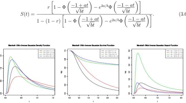
2.2.2 The Defective Gompertz Distribution

The Gompertz distribution is used for modeling survival data in various areas of knowledge

(Gieser et al., 1998), especially where there is a suspicion of exponential hazard. The

Gompertz density function is

f(t) =beate−ba(eat−1) (2.1)

for a > 0, b > 0 and t > 0. In this parameterization, a is the shape parameter and b is

the location parameter. The survival function is

S(t) =e−_ab(eat₋₁₎