A MODEL PREDICTIVE CONTROL FRAMEWORK FOR AUV FORMATION CONTROL
Rui Gomes∗,1Jo˜ao Borges de Sousa∗Fernando Lobo Pereira∗
∗Faculdade de Engenharia da Universidade do Porto, Rua Dr. Roberto
Frias s/n, 4200-465 Porto, Portugal
Abstract: This article concerns a Model Predictive Control (MPC) Framework for the control of AUV formations. The strict resource constraints - communications (which are acoustic), computation, and power - make the problem of decentralized control of AUV formations extremely difficult. Here, we present the first developments in the investigation of this problem. It involves the development of a simulation environment implementing a numerically efficient scheme based on a linear quadratic optimization problem. The next stage concerns the reformulation of this framework so that minimal information is exchanged.
Keywords: Model Predictive Control, Autonomous Underwater Vehicles, Formation Control
1. INTRODUCTION
Real world challenges that human kind perceives to-day, such as climate change, bio-diversity, environ-ment, natural resources manageenviron-ment, territory man-agement, security and surveillance, to name just a few, impose a number of increasingly sophisticated requirements for field studies data gathering. Spatial and temporal distribution, persistence, combination of wide area with local area data sampling, etc, are some general requirements calling for a concerted instrumentation of the earth which encompass net-worked fixed, mobile sensor platforms, and other de-vices. Moreover, one can easily devise many instances of missions involving, possibly heterogeneous, net-worked unmanned vehicles, say Autonomous Under-water Vehicles (AUVs), in which there is the need to distribute different sensors by different vehicles that should move in a certain formation defined to fulfill the needed data sampling requirements.
The underwater milieu poses tremendous challenges for the design of advanced data gathering systems. Onboard space and energy (required for the actua-tion, sensing, computaactua-tion, and communication) are at a premium and acoustic communications feature
1 The authors acknowledge the FP7 funding under the C4C
re-search project, and the FCT funding provided for the rere-search unit 147 - ISRP
very low data rates, are unreliable and power hun-gry. This makes the case for systems for which the overall management of onboard resources has to be carefully optimized. Moreover, hydrodynamic effects make precise models too complex from the computa-tional point of view and this implies that operacomputa-tional AUV models have necessarily to be approximated by simpler concentrated parameter models. The price to pay for this is that modeling becomes more difficult and uncertainty increases which is aggravated by the impact of typical pervasive underwater perturbations. In order to answer these challenges in the context of controlling a formation of AUVs tracking a given trajectory, a decentralized Model Predictive Control (MPC) framework is proposed.
Each vehicle runs an MPC algorithm that, by taking into account its own and its neighbors’ navigation data, generates a control strategy that balances a mini-mal quadratic error to the reference trajectory and de-viation from the pre-specified formation pattern with minimal employed control effort over time. Control and state constraints are also considered to reflect con-trol saturations as well as to avoid the collision with obstacles. The obtained control is applied for a short time interval, after which the state is sampled and in-formation is exchanged among the pertinent neighbor-ing vehicles via acoustic communication links. Then, the cycle is restarted with the new optimization carried
out over a shifted time horizon and with the most recent data.
The partiality of the information available to each AUV motivates a decentralized version of this prob-lem. However, this calls for a level of communication and of computation in each vehicle that strongly con-flicts with the available onboard resources. Thus, two main issues may arise in the networked MPC scheme. • acoustic communications may exhibit delays and
packets loss.
• computational complexity which, while taking into account the strict limitations of the AUV onboard resources, also has to meet real-time requirements.
A substantial amount of research work has been done on the control of formations of autonomous vehicles, (Franco et al., 2004; Franco et al., 2008; Keviczky et al., 2006; Keviczky et al., 2008; Fax and Mur-ray, 2004; Olfati-Saber and MurMur-ray, 2004; Semsar-Kazerooni and Khorasani, 2008; Goodwin et al., 2004; Fontes et al., 2009; Gruene et al., 2009; Allen et al., 2002; Liu et al., 2001). However, to the best of our knowledge, there are no satisfactory developments meeting the requirements of our applications.
This article is organized as follows: In the next section we discuss the various ingredients of the formation control problem and justify the options made. Then, in section 3, we present an overview of the state-of-the-art on MPC. In section 4, we discuss our decen-tralized MPC framework for the control of formations of AUVs and its implementation in a simulation envi-ronment. Finally, some brief conclusions are drawn.
2. AUV FORMATION CONTROL PROBLEM In this section, we formulate the AUV formation con-trol problem to concon-trol a set of vehicles that have to track a trajectory and, at the same time, keep a given formation pattern while satisfying state (safety re-quirements) and control (saturations) constraints. Typ-ically, modeling the AUV motion is difficult. Because of the hydrodynamic effects, AUVs are distributed parameter systems and, thus, represented by extremely complex models. For this reason, we use in our devel-opments the following model with coefficients based on results in (Prestero, 2001) and on our own field experiments. ˙η = u cos(ψ)− v sin(ψ) u sin(ψ) + v cos(ψ) r , (1) ˙ν = τu− (m − Yv˙)vr− Xu|u|u|u| m− Xu˙ (m− Xu˙)ur− Yv|v|v|v| m− Yv˙ τr− (Yv˙− Xu˙)uv− Nr|r|r|r| Izz− Nr˙ , (2)
whereη = [x, y, ψ]T (from here onwards, a “T ” in
upper script will denote transposed), ν = [u, v, r]T,
τ = [τu, τr], the coefficients Xu˙,Yv˙, Nr˙ represents
hydrodynamic added mass, Xu|u|, Yv|v|, Nr|r| the
hydrodynamic drag andm the vehicle mass.
From the above, we are interested in control strategies which, for each AUV i, i = 1, . . . , nv, minimize,
over a given time interval, a cost functional with two terms, one that penalizes the trajectory tracking error forcing vehicles to follow the desired path,ηi
ref, and
another that penalizes the control effort, thus saving the limited energy on board of vehicles, i.e.,
t+T Z t (ηi(s) − ηi ref(s)) TQ(ηi(s) − ηi ref(s)) +τiT(s)Rτi(s)ds, (3)
and, at the same time, satisfies the following:
(i) Kinematic and dynamic equations constraints (vehicle dynamics) given by (1) and (2); (ii) Endpoint state constraints,ηi(t + T )
∈ Ct+T;
(iii) Control constraints,τi(s)
∈ Ui;
(iv) State constraints,(ηi(s), νi(s))
∈ Si; (v) Communication constraints gc i,j(η i(s), ηj(s)) ∈ Cc i,j, ∀j ∈ G c(i); and
(vi) Formation constraints gfi,j(η
i(s), ηj(s))
∈ Cf
i,j, ∀j ∈ G f(i).
While the control constraints (iii) include, for exam-ple, saturations, the state constraints (iv) are specified to keep each vehicle in a specified set in order to satisfy safety or some other requirement. For example, to avoid collision with obstacles - known a priori or detected on the fly - or to prevent some variables to take on values that may damage components.
The satisfaction of the acoustic communication con-straints (v) ensure that the motion of the vehicles is such that the required connectivity is preserved. The fact that closer the vehicles are, the lower the power consumption and packets loss, makes a strong case for each AUV to communicate with its neighbors and, hence, for decentralized control structure. The com-munications structure may be described by the triple (gc, Cc,
Gc), where gc: Rn
× Rn
→ RM,Cc
∈ RM
(here,M ≤ n(nv−1)nv, beingn the dimension of the
state space component of interest of each vehicle), and Gca graph whoseithcomponent defines the vehicles
with which the ith vehicle communicates. We point
out that the communications graph is, in general, quite different from the formation or control graphs that we will introduce next.
Finally, the formation constraints (vi) specify the re-lations between data (typically, relative positions) of AUVs which have to be maintained with the help of appropriate control activity. These relative positions are specified in order to ensure the desired require-ments of the activity (e.g., data gathering) undertaken by the AUVs. The formation structure may be
de-scribed by triple(gf, Cf, Gf) where gf : Rn ×Rn → RM,Cf ∈ RM(here,M ≤ n(nv−1)nv, beingn the
dimension of the state space component of interest of each vehicle), andGf a graph whoseithcomponent
defines the vehicles with which theith vehicle has a
formation relation.
3. BRIEF STATE-OF-THE-ART ON MODEL PREDICTIVE CONTROL
There is an extremely vast body of literature on MPC -also designated by Receding Horizon Control (RHC) - that we cannot hope to include in this overview. See, for example, (Mayne et al., 2000). We will focus on the key results that are pertinent to our approach and focus on the class of systems addressed in this report -coordinated control of formations of vehicles. MPC is a control scheme in which the control action for the current time subinterval control horizon -is obtained, at each sampling time, by solving on-line an optimal control problem over a certain large time horizon - the prediction horizon - with the state variable initialized at the current best estimate updated with the latest sampled value. Once the optimization yields an optimal control sequence, this is applied to the plant during the control horizon. Then, once this time interval elapses, the process is re-iterated. The MPC scheme involves the following steps:
1. Initialization. Lett0be the current time, and set
up the initial parameters or conditions specifying x0, T , ∆, initial filter parameters (in case the
sampled data requires filtering, initial control for the recursive control optimization procedure, etc. 2. Sample the state variable at timet0.
3. Compute the optimal control strategy,u∗, in the
prediction optimal, i.e.,[t0, t0+ T ], by solving
the optimal control problem(P ).
4. Apply the obtained optimal control during the current control horizon,[t0, t0+ ∆].
5. Slide time by∆, i.e., t0 = t0 + ∆, and adapt
parameters and models as needed. 6. Go to step2.
wherex0is the initial state,T is the prediction horizon
for control optimization, and ∆ is the control hori-zon. A number of variants to this scheme have been considered by enriching some of steps with additional processing:
• For the networked systems implementation, the data obtained in step4. might be a composition of locally sampled data and data communicated from other vehicles or subsystems. For this class of systems, it might be of interest to replace data that failed to be transmitted by simulated data. • Filtering the sampled state variable is usually
required, being the Kalman filter widely used. • For situations in which models are significantly
uncertain or may vary over time, it might be of
interest to use the sampled data to identify or refine the value of model parameters.
• Likewise, if external perturbations act on the vehicles/systems are sensed or estimated, they can be used to improve the models entering in the optimization procedure, and to change the MPC parameters.
• Communication may introduce delays and data packets might fail to arrive with serious conse-quences to the controller performance. To ad-dress this, true data may be replaced by simu-lated data or MPC parameters may be adjusted. A typical general formulation of the optimal control problem(P ) may be as follows:
(P ) Minimize g(x(t0+ T )) + t0+T
Z
t0
f0(t, x(t), u(t))dt
subject to ˙x(t) = f (t, x(t), u(t)) L − a.e. u(t)∈ Ω L − a.e.
h(t, x(t))≤ 0 g(t, x(t), u(t))≤ 0 x(t0+ T )∈ Cf
where g is the endpoint cost functional, f0 is the
running cost integrand,f , h, and g represent, respec-tively, the vehicle dynamics, the state constraints, and the mixed constraints,C is a target that may also be specified in order to ensure stability. If one wants to take into account the uncertainty with respect to the initial state, then one may consider an initial state constraint, i.e., x(t0) ∈ Ci whereCi is an estimate
of the uncertainty set, being the minimization taken over the worst case of the initial state.
Now, we overview some of the typical basic issues and approaches for stability and robustness (Mayne et al., 2000; Langson et al., 2004; Mayne et al., 2009). Stability. Two major MPC approaches have been con-sidered to stability:
a) Direct method using the fixed horizon value function as a Lyapunov function; and
b) Indirect approach employing the monotonicity property of a sequence of value functions. Regardless of the approach, a number of formulations involving either a certain terminal state constraint set C, or terminal cost f0, or both, have been
consid-ered. In order to ensure the asymptotic stability of the obtained feedback control law, sayu = k(x), the required typical assumptions are:
• 0 ∈ C with C closed;
• k(x) ∈ Ω the control constraint set; • C is positively invariant under k(·); and • f0is locally a Lyapunov function.
Robustness. Robustness concerns the ability of the system in preserving a certain property - e.g., stability or performance - in the presence of uncertainties. For
stability, this can be checked by concluding that the Lyapunov function for the nominal closed-loop sys-tem keeps the descent property for sufficiently small disturbances. While this is not very difficult to show for unconstrained problems, the consideration of con-straints on states and controls raises substantial chal-lenges as it is required to ensure that the constraints remain satisfied. Inherent robustness, min-max open loop control and feedback control are the general contexts considered to investigate robustness of MPC schemes.
The versatility exhibited by optimal control problems has been exploited in order to formulate and solve problems of controlling formation of vehicles. These typically have a substantially complex structure and may be addressed by using MPC schemes in either a decentralized or a centralized context which may in-volve two stages: the planning phase - solved off-line to provide the formation reference trajectory -, and the execution phase - solved on-line with the help of locally formulated control problems. Let us overview a selected sample of some of these approaches. In (Franco et al., 2008), the problem of cooperative control of a team of distributed agents with decou-pled nonlinear discrete-time dynamics operating in a common environment and exchanging delayed infor-mation is considered. Each agent is assumed to evolve in discrete-time, based on locally computed control laws, which are computed by exchanging delayed state information with a subset of neighboring agents. The cooperative control problem is formulated in a receding-horizon framework, where the control laws depend on the local state variables (feedback action) and on delayed information gathered from cooperating neighboring agents (feedforward action). A rigorous stability analysis exploiting the input-to-state stability properties of the receding-horizon local control laws is carried out. The stability of the team of agents is then proved by utilizing small-gain theorem results. Building on the work reported in (Keviczky et al., 2006), a decentralized scheme for the coordinated control of formations of autonomous vehicles is pre-sented in (Keviczky et al., 2008). A high level reced-ing horizon control and coordination strategy is ob-tained for each vehicle by solving a LQ optimization problem featuring control saturation constraints, linear dynamics constraints, and formation constraints with neighboring vehicles defined by a graph. An appro-priate graph structure describes the underlying com-munication topology between the vehicles. On each vehicle, information about neighbors is used to pre-dict their behavior and plan conflict-free trajectories that maintain the coordination and achieve the team objectives. When feasibility of the decentralized con-trol is lost, collision avoidance is ensured by invoking emergency maneuvers that are computed via invariant set theory. A stabilization analysis is also discussed in (Keviczky et al., 2006).
Information exchange strategies that improve the for-mation stability and performance and, at the same time, are robust to changes in the communication topology are considered in (Fax and Murray, 2004) to address the problem of cooperative control of vehicle formations. The sensed and communicated informa-tion flow is modeled by a graph whose topology has implications in the control stability. By exploiting the interplay between communications and control, nec-essary and sufficient conditions for the stability of an interconnected system of identical vehicles can be derived. Stated in terms of the Popov criterium for net-worked control systems, these conditions involve the eigenvalues of the graph Laplacian and reveal how to shape the information flow in order to ensure stability and achieve high performance.
The problem of unreliable communication channel between the MPC controller output and the actuator input, has been addressed in, among others, (Gruene et al., 2009). Here, a mechanism for compensation of packet dropouts has been incorporated in the MPC scheme for discrete time problems. The basic idea consists in extending the control horizon until the next successful communication event happens and, in the meantime, use the best available control estimate, namely the one that has already been computed for the longer time interval. This article also includes some stability and sub-optimality analysis under an asymp-totic controllability assumption. In order to show sta-bility, the authors prove that, under the considered assumptions, the value function associated with the optimal control problem also exhibits properties of a Lyapunov function.
4. A DECENTRALIZED MPC FRAMEWORK FOR AUV FORMATIONS
In this section, we describe the implementation of a decentralized version of a discrete time MPC system to control a formation of AUVs in a simulation envi-ronment. The main features are:
• The decentralized character of the overall MPC controller is since each vehicle runs its own MPC scheme (which also encompasses the models of its neighboring AUVs) and communicates only with its neighbors;
• Computational efficiency is achieved by replac-ing the optimal control problem by a LQ opti-mization problem (for which an efficient MAT-LAB solver is used) and, for this, we consider (i) quadratic cost functionals, (ii) approximation of each AUV dynamics by a linear model, and (iii) state and control constraints (saturations) given by inequalities;
• Communication delays and packet dropouts can easily be incorporated; and
• Noise and disturbances can be easily considered in the vehicles simulated motion.
Now, we describe the optimization based control syn-thesis that will be performed in each AUV as part of the overall decentralized MPC scheme implemented in the simulation environment.
LetNp,nv, andT be, respectively, the prediction
hori-zon, the number of vehicles, and the sampling period. Then, according to the previous considerations, the discrete time linear model of vehiclei = 1, . . . , nv,
is, fork = 0, . . . , Np− 1, given by:
xi k+1= Φ i(T )xi k+ Ψ i(T )ui k, y i k = C ixi k (4) whereΦi(T ) = eAiT, Ψi(T ) = T Z 0 eAi(T −s)dsBi, andxi k ∈ R ns,u
k ∈ Rnc, andyk ∈ Rno are
respec-tively the system state, input and output variables, and ns,ncandnoare the associated space dimensions.
From the considerations of the formation control prob-lem formulation and assumed simplifications, it fol-lows that the underlying optimal control problem for AUV i, (LQPi), involves data from all its
neigh-boring vehicles as specified by the formation graph, consisting in minimizing the quadratic cost functional
Np X k=1 kyt+kref,i− y i t+kk 2 Qi+ Np−1 X k=0 kui t+kk 2 Ri + Np X k=1 X j∈G(i) kDij (yit+k− y j t+k)− d ij k2 Lij (5) subject to: xjt+k+1= Φ j(T )xj t+k+ Ψ j(T )uj t+k,(6) yjt+k= C j xjt+k (7) xjt+k∈ [xjLB,t, xjU B,t] (8) ujt+k∈ [u j LB, u j U B] (9) xjt = x j 0, (10)
where constraints hold for j ∈ {i} ∪ G(i), being, for each time k, G(i) the set of nodes of the graph specifying the vehicles linked to AUVi. Here, yi
t+k
andyref,it+k are, respectively, the vector of outputs of vehicle i and its reference, xj0 is the initial state of
vehiclej at the initial time t, Dijis a matrix reflecting
the formation relation between vehiclesi and j, dij
is a parameter vector specifying distances between vehicles i and j, xjLB,t, x j U B,t, u j LB, and u j U B are
bounds for state and control at timet, respectively. Now, we describe the implemented version of the MPC scheme for the control of a formation of AUVs. This scheme runs in each vehicle and will be the same for all AUVs. Thus, if there is no loss of information in the communication, then, all the vehicles have the same data and the control strategy generated for each vehicle is known to all of them. In the event of packet dropouts or communication delays, the missing sampled data is replaced by simulated data, and there will be some differences between the control strategies computed by the various vehicles for a given vehicle.
MPC Kalman Filter x ^ xref
Laboratório de Sistemas e Tecnologias Subaquáticas
Real Model (noise) Model Filter u x
Figure 3: Triangle formation simulation
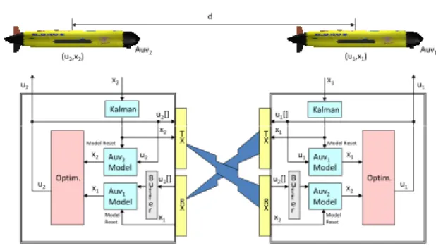
d Auv1 Auv2 (u2,x2) (u1,x1) u1[] x x1 u1 u2[] x x2 u2 Kalman Kalman Optim. Auv1 Model u1 x1 x2 Auv2 Model B u f f e r R X u2[] x2 T X x1 u1 Model Reset Model Reset Optim. Auv2 Model u2 x2 x1 Auv1 Model B u f f e r R X u1[] x1 T X x2 u2 Model Reset Model Reset
Figure 4: Triangle formation simulation
26
Fig. 1. Formation control scheme for 2 AUVs
The implemented MPC scheme in AUV i is as fol-lows:
1. Initialization: prediction and control horizons, other optimal control problem parameters that depend on specific mission requirements, such as, level of perturbations, existence of obstacles, relative importance of trajectory tracking and formation pattern errors.
2. Sample the state variable, compute its estimate, and communicate it to its neighbors via acoustic modem.
3. Obtain the state variable of its neighbors via acoustic modem.
(a) If data is available go to step4.
(b) Otherwise, generate estimates of the neigh-bors’ state by running their models. 4. Solve the linear quadratic optimization problem
(LQPi) at the current time t, and for the current
prediction horizon (of lengthNp) and the given
reference output trajectory. This yields an opti-mal control sequence for vehiclei.
5. Apply the control ui∗ for the current control
horizon.
6. Slide time for the optimization problem and ad-just parameters if needed.
7. Let time elapse until the end of the current con-trol horizon, and go to step2.
Simulation results were obtained with the developed simulation environment in which the MATLAB linear quadratic programming solver is used in the context of simple formation of two vehicles that have to travel side by side (see the diagram of figure 1).
This framework exhibits the following features: • Quadratic cost function weighting reference
tra-jectory tracking error, control effort, and forma-tion pattern error.
• Control systems with linear dynamics and sub-ject to Gaussian noise with “adjustable” mean and variance, added as an additional input in the vehicle dynamics. Once the vehicle state is sampled, a Kalman filter yields a state estimate which is fed in the optimization solver and com-municated to neighboring vehicles.
5.1: Com off 0 5.2: Com off 0.05
5.3: Com on 0.01 5.4: Com on 0.2
5.5: Com on 0.01 150 5.6: Com on 0.2 150
Figure 5: Simulations results
6.1: Com on 0.1 150m current=0.1 R=005 6.2: Com on 0.1 150m current=0.1 R=001
Figure 6: Current simulations results
7.1: Com on 0.1 obstacle avoidance, distance=0 7.2: Com on 0.1 obstacle avoidance, dis-tance=150m
Figure 7: Obstacle avoidance simulations results
Noise level Noise 0.00 0.01 0.05 0.10 0.2
COM M SOF F R = 0.01 T M etric F M etric Cost T M etricReal F M etricReal 6.48 0.31 106 6.48 0.31 6.46 0.32 106 5.82 1.01 6.29 0.34 108 8.14 1.55 6.30 0.35 110 9.74 1.62 6.33 0.34 112 10.7 1.69 COM M SON Distance = 0m R = 0.05 T M etric F M etric Cost T M etricReal F M etricReal 11.39 0.36 183 11.4 0.36 11.40 0.36 184 9.20 0.65 11.02 0.42 197 13.6 4.80 11.04 0.46 220 15.7 6.76 11.18 0.49 260 15.6 6.84 COM M SON Distance = 150m R = 0.05 T M etric F M etric Cost T M etricReal F M etricReal 11.4 0.36 183 11.4 0.36 11.4 0.36 184 9.85 0.80 11.20 0.41 191 22.6 7.02 11.22 0.45 201 28.5 11.4 11.30 0.46 215 25.0 10.3 28
Fig. 2. Formation of 2 AUVs with obstacle avoidance
Figure 8: Triangle formation simulation
Figure 9: Formation control of two vehicles in a side-by-side formation Noise level Noise 0.01
Distance = 150m R = 0.05 T metric F metric Cost 15.84 5.02 781 Distance = 150m R = 0.01 T metric F metric Cost 26.17 7.03 1214 Noise level Noise 0.01
Distance = 0m R = 0.05 T metric F metric Cost 35.70 0.50 531.54 Distance = 150m R = 0.05 T metric F metric Cost 46.4 0.49 648
??????????????????????????????????????????????? VER FIG The simulation result given all previous considerations are shown in picture 9.
Notes:
• red refers to vehicle 1, green refers to vehicle 2, + represents the reference, solid represents the feedback of the position where the vehicle thinks it is (model with noise/disturbances), o represents the real position when the control of the previous system is applied to this model. This model acts as a monitor of how far is the disturbed feedback system from reality. • the controller performance looks very good both in terms of trajectory tracking and formation • The same noise realization in all simulations for fair comparison
Control weights in 16 were tuned to achieve best performance. It is clear that more importance have been given to the formation keeping than to the trajectory tracking and the control. For instance if the equal weights were given, we would assist to a loss of performance in the formation keeping. The weight on the control allows us to be careful how energy is used.
several simulations as the next table shows.
29
Fig. 3. Formation of 3 AUVs with obstacle avoidance • Inequality state and output constraints. These en-able the incorporation of obstacles and the per-formance assessment the proposed MPC scheme with obstacle avoidance.
• Communication model. Communicated data is time stamped and may exhibit a time delay pro-portional to the distance between the vehicles ex-changing data. Gaussian random packet dropouts can also be considered. The MPC scheme was assessed in the presence of time delays. Each vehicle has a linear buffer enabling the reception of multiple data samples from other vehicles and whose implementation is described in the previ-ous section.
• Two performance metrics enabling to measure how far the AUVs are from the trajectory to be tracked and how far they are from the defined formation pattern, are used. These measures pro-vide a good assessment of the controller’s perfor-mance.
Figures 2 and 3 gives the reader an idea of the perfor-mance of the MPC controller in the considered cases.
5. CONCLUSIONS
Multiple simulations runs revealed that the proposed framework produced the intended control strategies according to the requirements. Many research chal-lenges remain in order to achieve the computational tractability for problems with more complex forma-tions and larger number of vehicles. This will require new ways of taking into account the decentralization character and are the subject of current research.
6. REFERENCES
Allen, M., J. Ryan, C. Hanson and J. Parle (2002). String stability of a linear formation flight control system. In: Procs 2002 AIAA Guidance, Naviga-tion and Control Conf., Monterey CA.
Fax, J. and M. Murray (2004). Information flow and cooperative control of vehicle formations. IEEE Trans. Automat. Control49, 1465–1476.
Fontes, F., D. Fontes and A. Caldeira (2009). Op-timization and Cooperative Control Strategies. Chap. Model Predictive Control of Vehicle For-mations, pp. 371–384. Springer Verlag.
Franco, E., L. Magni, T. Parisini, M. Polycarpou and D. Raimondo (2008). Cooperative constrained control of distributed agents with nonlinear dy-namics and delayed information exchange: A sta-bilizing receding-horizon approach. IEEE Trans. Automatic Control53, 324–338.
Franco, E., T. Parisini and M. Polycarpou (2004). Co-operative control of discrete-time agents with de-layed information exchange: A receding-horizon approach. In: 43rd Decision and Control Conf.. Vol. 4. pp. 4274–4279.
Goodwin, G., H. Haimovich, D. Quevedo and J. Welsh (2004). A moving horizon approach to networked control system design. IEEE Trans. Automatic Control49, 1427–1445.
Gruene, L., J. Pannek and K. Worthmann (2009). A networked constrained nonlinear mpc scheme. In: Procs European Control Conference, Bu-dapest, Hungary.
Keviczky, T., F. Borrelli and G. Balas (2006). De-centralized receding horizon control for large scale dynamically decoupled systems. Automat-ica42, 2105–2115.
Keviczky, T., F. Borrelli, K. Fregene, D. Godbole and G. Balas (2008). Decentralized receding horizon control and coordination of autonomous vehicle formations. IEEE Trans. Control Systems Tech-nology16, 19–33.
Langson, W., I. Chryssochoos, S. Rakovic and D. Mayne (2004). Robust model predictive con-trol using tubes. Automatica 40, 125–133. Liu, X., A. Goldsmith, S. Mahal and J. Hedrick
(2001). Effects of communication delay on string stability in vehicle platoons. In: Procs 2001 IEEE Intelligent Transportation Systems. Vol. 4. pp. 4274–4279.
Mayne, D., J. Rawlings, C. Rao and P. Scokaert (2000). Constrained model predictive control: Stability and optimality. Automatica 36, 789– 814.
Mayne, D., S. Rakovic, R. Findeisen and F. Allgower (2009). Robust output feedback model predictive control of constrained linear systems: Time vary-ing case. Automatica 45, 2082 – 2087.
Olfati-Saber, R. and R. Murray (2004). Consensus problems in networks of agents with switch-ing topology and time-delays. IEEE Trans. Au-tomatic Control49, 1520–1533.
Prestero, T. (2001). Verification of a six-degree of freedom simulation model for the remus au-tonomous underwater vehicle. Master’s thesis. MIT, WHOI. Cambridge, MA.
Semsar-Kazerooni, E. and K. Khorasani (2008). Opti-mal consensus algorithms for cooperative team of agents subject to partial information. Automatica 44, 2766–2777.