Optimal Definition of Ship Packs: a
Case Study in a Retailer Company
Paulo André Vilela Gonçalves Pereira
Master’s Dissertation
Supervisor: Manuel Augusto de Pina Marques
Mestrado Integrado em Engenharia Industrial e Gestão
Retailer companies work with Ship Packs representing the minimum quantity suppliers deliver to distribution centers and, thereafter, to stores. This parameter of the retailers affects several costs along the entire supply chain.
The current work was developed in a major retailer company and was branched in two main stages: the definition of Ship Packs through an optimization model, which entails the modeling of all the costs influenced by it, and the development of a Decision Support System to the retailer use whenever redefining Ship Packs with suppliers.
The project was conducted in the fresh and non food departments of the retailer and a model to optimize Ship Packs costs across the entire supply chain, including handling and safety stock at distribution centers and inventory, spoilage, markdown and extra handling at stores was developed. In addition, transportation and provision cost components were also included in the model.
Some products deal with sales patterns that have an intense period of sales within one year, which unbalances the needs of the supply chain by only having one Ship Pack for the entire period. In the present study, an automatic seasonality identification methodology was developed in order to study the implementation of a different Ship Pack within this period. Another drawn model was for the situation in which international suppliers deliver with cases and inners. Cases are big boxes containing inners inside it, which contains several units of the product. In order to take advantage of the bigger boxes, a methodology was established to send the case to stores with higher demand as well as in the seasonality periods.
The obtained results provided significant savings in both departments of the company. In the fresh department, a cost reduction of 9% was achieved as well as a 15% reduction in the non food department. The main savings were in the picking cost followed by spoilage and processing. In the non food department, the main savings were also at picking, but with an important reduction in the inventory cost. The seasonality model allowed, in products with seasonal sales’ patterns, a cost reduction of 3% for both departments when compared to the single optimization model. The case/inners analysis shows that international suppliers oversized Ship Packs and for the retailer an important cost reduction of 38% can be achieved for products dealing with these practices.
In order to translate the developed model into a business application, a Decision Support Sys-tem was developed as a web application. This tool is being used by the retailer company to redefine their Ship Packs whenever negotiating with suppliers.
The application was programmed to contain the developed optimization model in the back-ground, which is activated by the user using a web interface. Then, the application reads the database containing all the information from the products and executes the optimization model. Finally, the outcome is processed to allow an holistic view of the entire chain for each product by showing in which cost components did the most significant savings occurred as well as the recommended Ship Pack.
As empresas de retalho trabalham com quantidades mínimas que são transportadas pelos fornecedores até aos centros de distribuição e, destes, até às lojas. Esta quantidade mínima é designada por Ship Pack e é um parâmetro importante para os retalhistas por afetar vários custos ao longo de toda a cadeia de abastecimento.
O presente trabalho foi desenvolvido numa empresa de retalho e está dividido em duas etapas: a definição dos Ship Packs através de um modelo de otimização, que formula os vários custos da cadeia, e o desenvolvimento de um sistema de apoio à decisão para o retalhista usar sempre que definir os Ship Packs junto dos fornecedores.
O trabalho foi desenvolvido para o departamento de frescos e para o departamento não ali-mentar de um retalhista. Foram analisados vários custos ao longo de toda a cadeia de abasteci-mento, nomeadamente os custos de manuseamento e do inventário de segurança dos centros de distribuição e os custos de inventário, de quebra, de depreciação e de extra reposição nas lojas. Adicionalmente, foram também considerados os custos de transporte e de provisão.
Alguns produtos apresentam padrões de vendas que têm um forte período sazonal. Nestes casos, a existência de um único Ship Pack ao longo de todo o ano cria um desequilíbrio nas necessidades de toda a cadeia de abastecimento. Foi desenvolvida uma metodologia que permite a identificação de uma forma automática de períodos de vendas de maior volume com o objetivo de estudar a possibilidade de definir dois Ship Packs diferentes, um para o período sazonal e outro para o período regular de forma a reduzir os custos da cadeia. Uma outra particularidade do problema é que alguns fornecedores entregam os produtos em cases e inners, em que os cases são caixas maiores que contêm os inners dentro. De forma a tirar partido desta prática dos fornecedores, foi desenvolvida uma metodologia que envia os cases nos períodos sazonais e para as lojas com maior volume de vendas e os inners nas restantes situações.
Os resultados obtidos foram bastante significativos nos dois departamentos. No departamento de frescos foi obtida uma redução de custos de 9% e no departamento não alimentar de 15%. As maiores poupanças obtidas foram no custo de preparação no caso dos frescos. No caso do não alimentar, o custo de preparação voltou a ter um peso preponderante, juntamente com o custo de inventário nas lojas. O desenvolvimento de um modelo sazonal permitiu identificar poupanças de 3%, para produtos identificados como sazonais de ambos os departamentos, quando comparado com a utilização de apenas um Ship Pack ao longo do ano. Adicionalmente, o modelo de cases/in-nerspara fornecedores internacionais permitiu poupanças de 38% provando que nestes artigos a definição dos Ship Packs estava bastante desfasada das necessidades do retalhista.
De forma a traduzir o modelo numa aplicação de negócio, foi desenvolvido um sistema de apoio à decisão como uma aplicação web. Esta ferramenta está a ser usada pelo retalhista para ajudar no processo de definição dos Ship Packs junto dos fornecedores. A ferramenta foi desen-volvida usando uma interface gráfica que interage com o modelo de otimização. O utilizador final interage escolhendo os parâmetros e artigos a otimizar e o output é devolvido de forma a que os resultados possam ser analisados para uma futura negociação com os fornecedores.
First, I would like to thank my supervisor Professor Manuel Pina Marques for all the valuable insights during the development of this dissertation. The long conversations will be certainly saved as words of wisdom.
To Professor Pedro Amorim I am truly grateful for the given possibility to be part of this project. All the motivation, confidence and knowledge were crucial to this work. Above all, thank you for the friendship and for teaching me the real meaning of the word efficiency.
I am thankful to Paulo Sousa for the rigorous review of this work and for all the friendship during these last months. It was definitely funnier and interesting to work with you.
I am extremely overwhelmed for having met brilliant and inspiring minds at LTPlabs. They were a team responsible for part of my personal and work development. It is surely easier to work in a place like this.
Loads of memories have flourished in these last five years. This would have not been possible without my friends. Part of this thesis was developed with their support, guidance and friendship and, therefore, I would like to thank all of them for the greatest moments spent together.
To my little nephews for brighten my days with their guiltless joy. To my brothers for always caring about the youngest of the family and for being a continuous source of inspiration. To my parents for guiding my path and for always giving me the best.
Marta, without you all of this would have not been so shiny. Your continues care, support and friendship shaped the person I am today. Definitely the future looks brighter and worth to spend by your side.
Paulo G. Pereira
John Fitzgerald Kennedy
1 Introduction 1 1.1 Motivation . . . 1 1.2 The Project . . . 2 1.3 Dissertation Structure . . . 3 2 The Problem 5 2.1 Description . . . 5
2.2 The Proposed Approach . . . 10
3 Literature Review 13 3.1 Retail Supply Chains . . . 13
3.2 Warehousing . . . 14
3.3 Replenishment methods . . . 14
3.4 Bullwhip Effect . . . 15
3.5 Fresh Food on Retailing . . . 16
3.6 Ship Pack Optimization . . . 16
3.7 Seasonality and Stores Clustering . . . 19
4 Methodology 21 4.1 Model Formulation . . . 21
4.2 Seasonality Identification . . . 30
4.3 Stores Clustering . . . 32
4.4 Ship Pack Optimization . . . 33
5 A Case Study in a Retailer Company 37 5.1 Cost Modeling Results . . . 37
5.2 Ship Pack Optimization Results . . . 40
5.3 Global Results . . . 45
6 The Decision Support System 51 6.1 Requirements Definition . . . 51
6.2 DSS Architecture . . . 52 7 Conclusions and Future Work 57 A Store Inventory Demonstration 63 B Case/Inner Analysis 65
C DSS Interfaces 67
DC Distribution Center DSS Decision Support System PBL Picking by Line
PBS Picking by Store SKU Stock Keeping Unit
1.1 Project’s timeline . . . 3
2.1 Stakeholders impacted by the Ship Pack Definition . . . 5
2.2 PBL and PBS flows . . . 6
2.3 Processing Cost from the Fresh Department . . . 6
2.4 Processing Cost from the Non Food Department . . . 7
2.5 Costs affected by the Ship Pack in every stage of the Supply Chain . . . 9
4.1 Inventory Position and On-hand Stock . . . 22
4.2 Store Inventory Cost Modeling . . . 26
4.3 Shrinkage Parameters . . . 28
4.4 Sales patterns for different SKUs . . . 30
4.5 Seasonality identification for different SKUs . . . 32
4.6 Percentage of periods supplied by Cases . . . 33
4.7 Ship Pack optimization matrix . . . 33
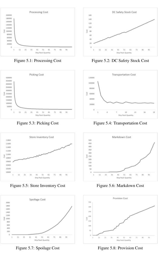
5.1 Processing Cost . . . 39
5.2 DC Safety Stock Cost . . . 39
5.3 Picking Cost . . . 39
5.4 Transportation Cost . . . 39
5.5 Store Inventory Cost . . . 39
5.6 Markdown Cost . . . 39
5.7 Spoilage Cost . . . 39
5.8 Provision Cost . . . 39
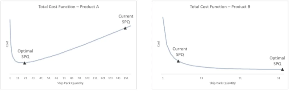
5.9 Total Cost Function 1 . . . 41
5.10 Total Cost Function 2 . . . 41
5.11 Product A - Optimization Result . . . 41
5.12 Product B - Optimization Result . . . 41
5.13 Seasonal product sales . . . 42
5.14 Seasonal Ship Pack Optimization . . . 42
5.15 Ship Pack Optimization - Cases/Inners . . . 43
5.16 Extra Handling Cost . . . 43
5.17 Extra Handling Cost Sensitivity . . . 44
5.18 Ship Pack for Boxes and Pallets . . . 44
5.19 SPQs variations in the Fresh Department . . . 47
5.20 SPQs variations in the Non Food Department . . . 47
5.21 Products’ ABC . . . 49
5.22 Suppliers’ ABC . . . 49
5.23 Unit’s deviation . . . 50 xiii
5.24 Period of sales deviation . . . 50
6.1 DSS Architecture . . . 53
6.2 Solver Architecture . . . 53
6.3 Homepage . . . 54
6.4 Solver Debug . . . 55
A.1 Inventory Position and on-hand stock . . . 63
B.1 Single optimization model vs Case/Inner . . . 65
C.1 Log In . . . 67
C.2 Homepage . . . 68
C.3 Cost components parameters . . . 69
C.4 Run Optimization . . . 70
C.5 Input of the Model . . . 71
C.6 Log from the Ship Packs Optimization . . . 71
C.7 Output of the Model . . . 72
C.8 Run Optimization Validation . . . 73
C.9 Pre-validation Seasonality . . . 74
C.10 Data Pre-validation . . . 75
C.11 Item-like for new Ship Packs Optimization . . . 76
C.12 Market’s structure for new Ship Packs Optimization . . . 76
C.13 Output for new Ship Packs Optimization . . . 77
C.14 File for new Ship Packs Optimization . . . 78
C.15 Input file for new Ship Packs Optimization . . . 78
C.16 Output file for new Ship Packs Optimization . . . 79
C.17 Supplier’s Ship Packs Optimization . . . 79
C.18 Input for Supplier’s Ship Packs Optimization . . . 80
2.1 Costs affecting each Commercial Department . . . 9
2.2 Proposed Approach . . . 11
4.1 Table of Notation . . . 23
5.1 Supplier Optimization . . . 45
5.2 Products from each Department . . . 46
5.3 Results from the Single Optimization Model . . . 46
5.4 Results from the Seasonality vs Single Optimization models . . . 48
5.5 Results from the Case/Inners Optimization . . . 49
Introduction
“ The system of people and things that are involved in getting a product from the place where it is made to the person who buys it”
Supply Chain Definition from Cambridge Dictionary
1.1
Motivation
Retailer companies face numerous challenges in supply chain management by balancing to-gether efficiency and flexibility toward a quick response to demand needs. Companies dealing with supply chains, with an holistic view of it, tend to diminish the chances of jeopardize their business activities through the creation of long term sustainability and market leadership. Thus, supply chains have become a key to secure a competitive advantage against other players in the market.
The amount of stakeholders retailers’ companies deal with has considerably grown up in the past years, turning retail business into a challenging tangled network burdensome to manage. Therefore, supply networks from major retailers are designed to integrate logistics operations into central warehouses, which consolidate and distribute goods to stores. Distribution centers (DCs) can be seen as an order fulfillment center allowing the stocking of goods for a period of time until the next order arrives followed by the consolidation of all the ordered goods, which are then delivered to stores.
These kind of networks entails troublesome challenges in combining production from suppli-ers with low inventory levels at the several echelon stages, distribution centsuppli-ers and stores, together with an enhancement in customers’ sales. This leads to a tenacious focus on the net margin by increasing sales and at the same time scale down costs through more flexible and efficient supply chains. The ultimate goal of a retailer is to strengthen sales by allocating the right product to the right place to the right customer at the right time together with an escalation in the net margin.
The distribution starts with suppliers packaging the produced goods in boxes/pallets containing several units of it. The same quantity is maintained until the end of the chain where the package
is finally opened at stores. This is called the Ship Pack and represents the minimum quantity suppliers deliver to distribution centers and, thereafter, to stores.
This parameter of the supply chain, in spite of not being deeply studied, affects several costs and stakeholders along the entire chain. It can be unbalanced with demand needs, leading to additional efforts of the chain and, as consequence, to a decrease in the closing margin.
In Van Zelst et al. (2009), the most important drivers of operational logistical costs are figured out. The costs included transportation, inventory and handling, both at warehouses and stores, and the results lead to the identification of Ship Packs as an important driver to these costs. Therefore, an appropriate definition of it leads to an increase in efficiency, in the retailer’s supply chain, by minimizing the costs across the entire chain.
Normally, the Ship Pack is negotiated with the supplier and until the next negotiation it keeps unchanged. Due to this hard constraint, its definition gains an utterly importance as it is challeng-ing to settle a different one with suppliers until the next round of negotiation occurs.
An appropriate Ship Pack definition can lead to an optimized cost chain for each product. On the assumption of a cost reduction for a significant portion of the overall products, its redefinition may lead to large-scales savings and, consequently, to an increase in the obtained margin.
1.2
The Project
The present study was developed as part of a consulting project in a national retailer company in order to determine the optimal quantity of the Ship Pack in the whole chain for several Stock Keeping Units (SKUs) the company deals with. The need of the project arose as the company was clueless with the impact Ship Packs have on its operations and wanted to have a model capable of indicating the optimal Ship Pack according to their needs in order to redefine it during negotiations with suppliers.
The key stakeholders of this project were the non food and fresh commercial departments of the company as they were the ones responsible to perform tactical decisions and negotiate with suppliers. However, as the project is transverse to the entire supply chain, several other teams were included in the project in order to model all the costs impacted by the Ship Pack definition.
In order to perform an holistic approach to this problem, the several stages of the retailer’s chain, such as DCs and stores, have to be included in the scope of this project. The retailer has several stores, all over the country, which are mostly daily supplied with goods from the DCs according with the type of product. The company has several distribution centers: three for non-food products, four for fish, meat, codfish and bread, which are also responsible to process products, and two dealing with most of the remaining food products. The scope of this work includes all the distribution centers and stores.
The final goal is to provide the company with an optimization-as-a-service by developing a Decision Support System (DSS) available as an online application including the developed opti-mization model.
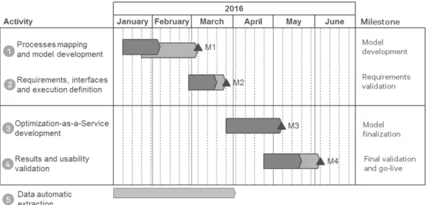
The project is branched in two main stages. The first step is the definition of Ship Packs through an optimization model as seen in figure 1.1, which entails the modeling of all the costs influenced by the Ship Pack. The second step involves the development of a Decision Support System for the retailer use whenever redefining Ship Packs with suppliers. This includes an ex-tensive requirements and interfaces validation followed by the tool development and, finally, by the end user validation of the results. This can bee seen in activities 2, 3 and 4 from the project’s timeline in figure 1.1.
As the DSS is supposed to automatically receive the necessary data from the company’s database, there was another project running indoors the company to create automatic data ex-traction procedures and maintain the tool live without using data manual inputs from the users. This can be seen in detail in the last activity of the project’s timeline.
Figure 1.1: Project’s timeline
1.3
Dissertation Structure
The dissertation is structured as follows. In Chapter 2, the impact of Ship Packs in the whole chain is tackled by analyzing all the stages affected by it as well as the proposed approach to cope with the stated problem. In Chapter 3, past works dealing with similar optimization problems were studied, as well as existing gaps in the current literature are presented. In Chapter 4, an optimization model is designed to minimize the costs related with Ship Packs considering the most imperative factors in the whole chain. Chapter 5 presents the results of the develop method in the particular case of the studied retailer company. In Chapter 6, the requirements, interfaces and usability of the DSS are described including the necessary tools to design and build it from scratch. In Chapter 7, the main conclusions are drawn and future enhancements to the work developed are discussed together with possible add-ins to the developed DSS.
The Problem
The definition of Ship Packs is a multiple variable problem leading with linear and non linear cost expressions, which affect differently each piece of the supply chain. Hence, in order to properly define the impact of its definition in the supply chain, all costs have to be considered and the optimal Ship Pack is achieved by minimizing the developed cost function. An holistic approach has to be followed in order to define the optimal quantity, which includes an analysis of the entire chain, starting with distribution centers, followed by transportation and stores as seen in figure 2.1. The Ship Pack definition also impacts the supplier in their production and distribution. However, the developed model will only focus on the internal costs of the retailer.
Figure 2.1: Stakeholders impacted by the Ship Pack Definition
2.1
Description
Distribution Centers
The distribution center is the warehouse where the retailer receives the goods from suppliers, which are then delivered to stores.
The warehouse is organized in two primary flow types: Picking by line (PBL) and Picking by Store (PBS) as seen in figure 2.2. PBL is a flow type dealing with zero stock in which goods arrive from suppliers and are placed in fixed positions representing each store. When all the goods are picked to the corresponding place, the order is shipped to the destination. This operation is related with suppliers who have high service levels and work with just-in-time operations as goods are usually shipped from the distribution centers in less than one day.
On the other hand, PBS - Picking by Store, is a flow type dealing with stock. The SKUs are located in fixed positions and the picking is done by collecting the SKUs from its position when an order is placed. The picker, person responsible to collect the SKU, moves around the racks and collects all the SKUs associated with the store’s order. The fixed position is associated with the SKU, contrary to the PBL operation in which stores’ position is fixed.
Figure 2.2: PBL and PBS flows
At the distribution center, the two main costs components are linked with handling costs, which can be split into processing and picking, and inventory costs. As this project was conducted in the fresh and non-food department of the retailer company, there were some differences in the cost process modeling for both departments.
Considering the fresh department, processing deals with the place of the received goods, which are gathered in big boxes, to small and standard boxes that will be the shipment unit for the remainder chain. This operation occurs mainly with fish, meat and bread products.
Figure 2.3: Processing Cost from the Fresh Department
In the case of the non-food department, some of the received goods arrive from international suppliers who send it in big boxes (Cases) containing small boxes (Inners) inside it. After arriving into the warehouse, the cases are opened and placed upon pallets to be stocked into the ware-house. This implies that, currently, only inners are sent to stores and cases are only used until the warehouse.
The processing cost for both departments is expected to decrease with larger Ship Pack as less boxes will be processed.
Figure 2.4: Processing Cost from the Non Food Department
Picking is another cost associated with distribution centers. In this situation, the cost is linked with the movements workers have to perform in order to collect the ordered SKU from its position in the warehouse. In both departments, picking movements are similar and the only difference is the picking cost, which changes according to the corresponding distribution center. Analogous to the processing cost, the picking cost is expected to decrease with larger Ship Packs.
As mentioned before, there is only stock of goods in the PBS flow type operations. Therefore, in the SKUs related with PBL operations, the Ship Pack definition does not influence the DC inventory cost. Moreover, in products leading with PBS operations, a larger Ship Pack will result in larger order quantities by the stores as orders will be less frequent. Hence, the DC is expected to have a larger safety stock in the situations where the Ship Pack increases. This happens because the DC has to maintain the same service level to stores in order to pay off the larger variance due to the bullwhip effect.
Transportation
There are some products in which the Ship Pack is a standard box meaning that all the mea-sures and maximum carried weight are known. This is contrary to the situation in which the sup-plier uses a box without standard measures and the information about the available boxes being used is not provided.
Whenever using standard boxes, there is a list of possible boxes and on these terms it is attain-able to indicate the most appropriate standard box to a better usage of it considering the product’s weight, dimensions and the Ship Pack quantity.
The driver of the transportation cost is the number of carried pallets. A balanced Ship Pack might lead to a better utilization of the transportation box and, therefore, less boxes are carried. Potentially, this means less carried pallets and a reduction in the transportation cost is expected.
This cost can only be derived if the transportation is done with standard boxes in which the number of boxes and pallets can be calculated. In the situations of non standard boxes, the trans-portation cost can not be calculated as there are non standard measures for the used boxes.
Stores
The final stage of the chain are stores where several costs components are influenced by the Ship Pack definition.
Analogous to the distribution center, there is also an inventory cost influenced by the Ship Pack as orders have to be multiples of it. This leads to situations in which expected demand is below the rounded up order pointing to an extra stock as a result of the residual units not being sold. Larger Ship Packs tend to less replenishments from stores as larger orders are made. Considering the stores’ replenishment methods to order goods from DCs, the average inventory, in each store, can be estimated by rounding up the order quantity to a multiple of the Ship Pack quantity.
Some inventory fluctuations are expected as sometimes the Ship Pack, even though being larger, might lead to a smaller order quantity because it can be an exact multiple of the Ship Pack and, consequently, less units are ordered. Therefore, the stores’ inventory cost is expected to have some fluctuations upon the Ship Pack quantity.
When an order arrives to the store, the product is fitted into the store’ shelves until these are completely full. There is a cost of shelf stocking, which according to Sternbeck (2015), includes the following procedures: picking up the Ship Pack, identify the SKU, opening the box, walking to the shelf and looking for the slot on the shelf. However, not all the units fit on the shelf and the remainder units of the product return to the backroom and await for the next shelf filling. This extra movement incurs into additional costs, which are dependent on the Ship Pack size. Small quantities of it lead to a better fit into the shelf and, consequently, larger Ship Packs are expected to increase the store extra handling cost.
Shrinkage costs according to Beck et al. (2002) can be due to product going out of date or under pricing. Spoilage is normally referred to losses due to expiration dates and markdowns to under pricing when the product is near expiration dates.
In the fresh department, most of the products are perishable with short expiration dates and as Ship Packs influence the inventory in stores, the spoilage cost is expected to increase with larger quantities of it. In addition, this issue was one of the motivations behind the current project as a myriad of SKUs were having spoilage costs due to an unbalanced Ship Pack definition.
In order to avoid shrinkage, some SKUs have a markdown when close to expiration dates. According to Ferguson et al. (2007), managers frequently utilize markdowns to stabilize demand as the product’s expiration date nears. This cost is also expected to be influenced by the Ship Pack in similar ways as the spoilage cost.
The utmost cost component is a very particular one related with the considered retailer and it is associated with a financial penalization of slow movers products having long standing stocks. This cost is called provision and it is only calculated with products from the non food department and it is expected to increase with larger Ship Packs.
In figure 2.5 all the costs are bond together and this will be the groundwork of the current project in the following chapters. It is important do denote that most of the products follow this supply chain, but a few of them are directly supplied to stores by suppliers. On these terms,
the distribution centers will be excluded from the analysis and only the costs upon it will be considered.
Figure 2.5: Costs affected by the Ship Pack in every stage of the Supply Chain
Table 2.1 summarizes how each cost affects respectively the studied departments and the par-ticularities of each one. These different characteristics between both departments will be consid-ered when modeling all the costs of each SKU. These idiosyncrasies can change the cost function or work as a binary value to whether or not consider the corresponding cost component in the total cost function.
Table 2.1: Costs affecting each Commercial Department
Cost Fresh Department Non Food Department Picking Includes both PBS and PBL flowtypes
Safety Stock Few PBS operations Mainly PBS operations Processing Changing products to another boxes Opening cases and palletizing Transportation Standard and supplier’s boxes Only supplier’s boxes Store Inventory Depends on the store’s replenishment method Extra Handling Depends on the store’s shelf space
Spoilage Short expiration dates Few expiration dates Markdown Includes markdowns No markdowns
Provision No penalization of stocks Penalization of longer stocks
Demand Variability Analysis
Together with the costs considered in the above stages, there are some other variables affecting the Ship Pack definition. The goal is to study and quantify how does these variables might deeply affect the cost of the entire chain and whether or not it is worth it to change the current situation.
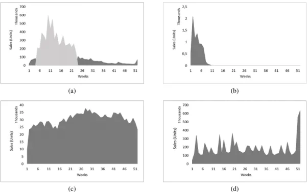
A product might not sell equally throughout the year. Some products might have strong de-mand peaks in which sales are strongly above average in comparison with regular periods. This does not mean punctual promotions, but long periods of strong sales such as school products that have a peak of sales occurring in the beginning of the school period. Therefore, the same Ship Pack during all year is unbalanced and the effort of having two Ship Packs for different periods
in time, which entails negotiating with the supplier, might be justified if there is a considerable cost reduction on this approach. The same happens with seasonal fruit products that sell through the entire year, but have an intensive demand period due to customer’s consumption (ex: Melon during summer) or to product’s production (ex: Strawberry).
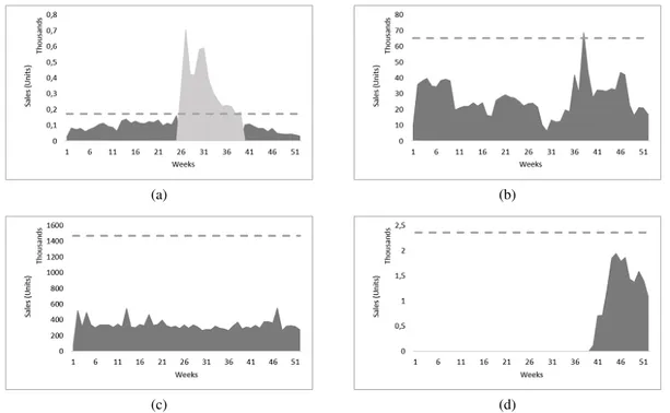
This leads to the precondition of identifying the seasonality period from a demand history anal-ysis and, consequently, introduce a different Ship Pack into the model for this period of time. The goal is to provide an outcome identifying the seasonal and regular periods and the corresponding Ship Packs.
In addition, as the retailer company encompasses several stores with different sales patterns, this different sales’ volume within stores might justify the implementation of two Ship Packs for different stores based on their sales history. However, having two Ship Packs references at the same time leads to the need of having two picking references at the warehouse and, in the current moment, the capacity of most of the distribution centers does not allow this kind of operation.
As mentioned before, some of the products are shipped using cases and inners and in order to take advantage of this obligation from the supplier, it was decided to study the implementation of sending the case in the situations of larger demands such as seasonality periods or to stores with higher sales.
Stores with higher sales will be identified through a demand history analysis and be associated in two groups. One of the groups will be supplied by inners and the other with cases.
Altogether, demand variability within stores and demand peaks through a period of time might justify the effort of having different Ship Packs to diminish the chain’s costs.
2.2
The Proposed Approach
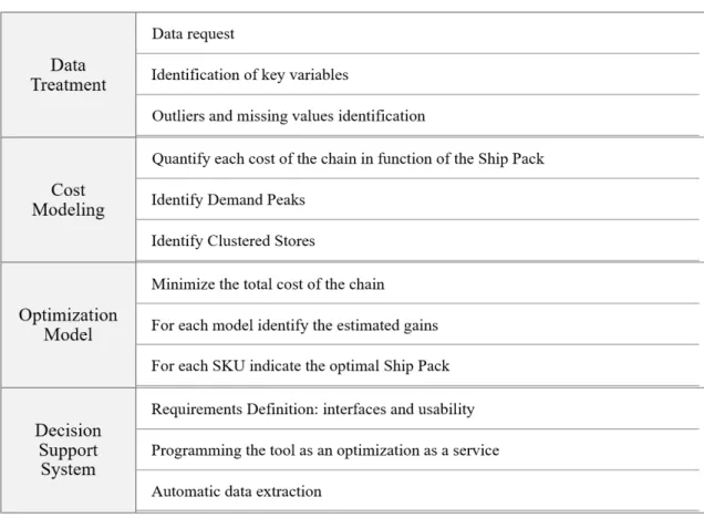
The proposed approach follows a four fold methodology as seen in table 2.2.
In the first step there will be a strong focus on the data treatment starting by an extensive data request to the company’s information technology department. Then, data identification and understanding will lead to a special treatment of outliers and missing values to keep the model coherent and rigorous.
The second step is the cost modeling for each of the mentioned cost in function of the Ship Pack quantity. In addition, with the sales history it will be possible to identify whether or not the product has significant demand peaks and if there is a strong demand variability among stores.
The third step is related with the optimization of the cost function and it proposes to indicate the optimal Ship Pack for each SKU of the company as well as the estimated gain for the developed model.
The final step proposes the development of a Decision Support System as an optimization as a service available online for each department of the retailer in order to indicate the best Ship Pack quantity for each SKU. It entails a requirements phase in which interfaces and usability need to be defined followed by the development of the tool, which is going to be fed by an autonomous data extraction maintaining data updated over time.
The current project will address mainly step two and three by giving a stronger emphasis to the cost modeling and, consequently, to the optimization model as these are the core components of the project. However, the data treatment played an important role as the project dealt with a huge amount of data and the DSS worked as way to transfer the developed knowledge into a business application.
Literature Review
The goal of this chapter is to induce the reader into the current state of the art in the Ship Pack optimization by covering all the stages of the supply chain and how the Ship Pack influences it. The literature review is organized as follows. In section 3.1, an introduction to retailers’ supply chain in a broad manner is made as an intent to contextualize the current problem into the supply chains current needs and challenges. In section 3.2, distribution strategies and picking policies are covered in order to detail how central distribution is currently organized. In section 3.3, the impact of shrinkage costs in fresh products are analyzed including spoilage and markdowns costs and how the perishable products have different particularities when compared with the remaining products. The bullwhip effect and its repercussions in the coordination of the chain are stated in section 3.4. The current replenishment methods are covered in section 3.5 followed by an explanation of the current practices in stock management. In section 3.6, the state of the art in the current Ship Pack optimization is addressed as well as possible gaps in the existing research. Finally, in section 3.7 some definitions about seasonality identification and clustering are addressed in a broad manner.
3.1
Retail Supply Chains
The importance of supply chains in the retail business is addressed in Fernie and Sparks (2014). From a customer perspective, it is often forgotten the effort retailers made in order to place the desired products on shelves. Handling with variability in demand, due to customer’s changes in beliefs and needs, is a challenging task as a bad prediction might lead to a disruption in stock or to an extra stock. Therefore, forecast needs to be balanced with sales and all of the logistical processes in order to guarantee the availability of the product when customers are buying it.
Fernie and Sparks (2014) also states that current retailers have been concerned to ensure dis-tribution channels are both anticipatory and reactive to demand’s changes. Although right product availability is the main goal of a retailer there are some issues contributing to the efficiency of the chain. Holding excessive stock, both at warehouses and stores, is a costly activity as stock might become obsolete or deteriorated due to expiration dates. In addition, there is also the cost of trans-porting goods from suppliers to warehouses and then to stores, which also needs to be balanced.
An efficient chain can lead to less costs and, potentially, the retailer might look more appealing to the customer’s perspective as prices may go down. Therefore, dealing together with demand and supply though excelled information systems can lead to a better service to customers as it can provide fresher and higher quality products minimizing the risk of stockouts.
3.2
Warehousing
There are two main distribution strategies: traditional warehousing and cross-docking. In the first one, retailers keep stock at Distribution Centers and when customers or stores request a product, the item is picked from the racks (Li et al., 2008). This works in an analogous way to the PBS flow type mentioned in the previous chapter.
On the other hand, cross-docking is a distribution strategy where distribution centers function as an inventory coordination point rather than an inventory storage point (Waller et al., 2006). This is compared to the PBL flow type because there is no safety stock at the distribution center. How-ever, the two operations are distinct because cross-docking implies the product transfer to another vehicle when the product arrives into the DC and the PBL flow type includes the reorganization of all the products by store before sending it to the store.
In Benrqya et al. (2014), the impact of product characteristics on distribution strategy selection is studied in several categories. The aim is to, according with the product, market and supply factors, choose the best distribution strategy either from traditional warehousing or cross-docking. This work is indirectly related with Ship Pack definition as some of the mentioned factors are dependent from the Ship Pack size, which may indirectly lead to the choice of the best distribution strategy making this as a pivotal consideration along the entire supply chain.
De Koster et al. (2007) defines order picking as the process of retrieving products from storage (or buffer areas) in response to a specific customer request. It is classified as the most labour inten-sive operation in warehouses. It also states the importance of warehouses to achieve transportation economies, consolidation of orders and deal with demand’s uncertainty among many other factors. Tompkins et al. (2010) describes the first step in the warehouse flows as the reception of the goods from suppliers followed by either it storage or shipping immediately, which makes the warehouse working as a cross-docking platform. The storage can be divided in two: reserve storage with pallet picking or case picking. After storage, an order is made and replenishment is made to the shipping area.
A comparison between picking, storage and routing policies is performed in Petersen and Aase (2004) and results show orders’ batching contribute significantly to the greatest savings, particularly when smaller order sizes are common.
3.3
Replenishment methods
In Wagner (2002), the evolution of inventory models is analyzed. The earliest publications date back almost one century ago and referred to Economic Order Quantity (EOQ), which is still
studied nowadays. Back to this time, the main difficulties were related with the attainment of historical demand data and empirically test stock models due to lack of computing power.
Brown (1959) targets inventory modeling in two main issues: the time to replenish inventory and what should be the order quantity. It states the order must occur when the current inventory does not reach the targeted service level and the quantity must be enough to cover the forecast demand until the next order arrives.
Wagner (2002) also focuses on why stock outs continue to occur, even though technology development lead to a better use of inventory models. Some of the problems stated are related with demand not being leveled across the year as well as when new SKUs are introduced there is not enough data to extrapolate solid conclusions and there is also laborious to differentiate stock outs due to bad stock management or suppliers’ failure.
The two most common stock management practices are are inventory continuous and periodic review. Continuous review indicates that inventory status is tracked in a continuous way and the order is made to a certain quantity designated as Q. On the other hand, periodic review indicates that inventory is tracked at regular periodic intervals known as R and a reorder is made during the review period to raise inventory to a predefined level (Chopra and Meindl, 2007).
3.4
Bullwhip Effect
According with Lee et al. (2004) when the retailer’s orders do not coincide with the current retail sales, a distortion in the demand information had occurred leading to a larger variance from orders than from sales. This lead to a demand amplification upstream the chain and in a multiple echelon stage, like a retailer’s supply chain, it is frequently quoted that the amplification can be more than the traditional 2:1 affecting several echelons and leading to extra stock costs to avoid stockouts and completely fulfill the expected demand.
The traditional and most common explanation to justify the bullwhip or whiplash effect is the lack of information between stages in the supply chain. Geary et al. (2006) did an extensive work to cover the ten principles leading to bullwhip reduction. One of those principles, in the interest of this study, is the order batching principle, which is influenced by Ship Pack definition as it leads to "lumpy" deliveries, and hence come back around the ordering loop.
In Yan et al. (2009), the effect of delivery pack size in the bullwhip effect was studied and found significantly correlated with larger pack sizes. It concludes that the increase of pack size forces the retailer to order less frequently but in larger quantities leading to the amplification of the demand at the distributor level. In addition, the average stock on hand rises significantly due to order-rounding rule particularly when the minimum order quantity is much larger than demand during the review period.
3.5
Fresh Food on Retailing
Fresh products account for a large part of retailer’s revenues and are also strong drivers of store’s traffic and customer loyalty. In Raphael Buck (2013), the most critical dimensions for successful fresh retailers are stated and it included supply chain and shrinkage reduction as two of the main factors. Shrinkage is defined as the cash value of products that a retailer has bought that are not sold due to expiration dates or to under pricing. Opportunities to reduce shrinkage can be found in every part of the supply chain including the inadequate shelf space or the replenishment process.
The shelf space is related with the quantity a product has allocated on a shelf and in most of the times there is no analytic rule to define the optimum quantity. This unbalanced allocation might lead to the deterioration of products that are not sold. The replenishment process may lead to an extra stock that is not required and, consequently, to an over cost due to shrinkage.
In Van Donselaar et al. (2006), a study was conducted in two Dutch supermarkets analyzing the difference between perishable and non-perishable products. Based on this, shelf life, average weekly sales, coefficient of variation for weekly sales, case pack size and average time between two replenishment orders were found to be clearly different for both sort of products. In the situation of the case pack size, the median was 6 and 10 for perishable and non perishable products, respectively. In the remainder of the paper, a different control of inventory to perishable products is formulated in order to compensate the differences between the two range of products.
In addition, most of the retailers tend to use markdowns to stabilize demand as expiration date nears. In Ferguson et al. (2007), most of the perishable products are stated to have two markdowns for each batch. The first one occurs at half of the product’s life time and is typically 10-50% of the product’s original price. The second markdown occurs at 75% of the product’s life time and is typically 25-75% of the original price. Retailers use this dynamic pricing technique to stabilize demand as consumers are expected to buy less products near expiration dates unless there is a reduction in the original price.
3.6
Ship Pack Optimization
The motivation to study the Ship Pack definition is well addressed in Van Zelst et al. (2009) as size pack definition is clearly demonstrated to be an important driver for stacking efficiency. In the presented study, costs are subdivided in inventory and handling, both at warehouses and stores, and transportation. Handling costs represent by far the biggest pie in the total cost (66%), followed by transportation (22%) and leaving inventory to only 12% of the total cost. It concludes there is a need to balance Ship Pack size with handling costs and inventory costs as both costs fluctuate differently with different Ship Packs dimensions.
Hellstrom and Saghir (2007) provides an overview between packaging and logistic processes in the retail supply chain. It states packaging can lead to benefits in the logistic activities such as re-duction of handling activities and picking times, inventory carrying cost and the warehouse layout
could also be improved. Many packaging dependent costs in the logistics system are frequently overlooked, which included several logistic activities such as transport, inventory, warehousing and communication. In transportation, packaging decreases handling costs and loading times. In inventory, it increases product availability (sales) and decreases carrying costs. In warehousing, decreases order filling time, labour costs and material handling costs. In communication, decreases communications to track down lost shipments.
Waller et al. (2008) studied if case pack quantity affects significantly firm market share by analyzing product rate-of-sale by a regression analysis. These findings lead to the result of case packs quantities affecting market share due to less stockouts. It states two opposite effects of case pack quantities: (1) larger quantities reduce replenishment’s frequency and, consequently, less stockouts and (2) increase the probability that some units might need to be stored in the backroom as they do not fit on the shelf and, consequently, the number of exposures to stock outs increase.
Wang (2010) says that outer and inner packs can be ordered by the DCS if the outer is opened at the DC. This has benefits because it provides flexibility to meet the store’s demand even with an additional cost. It develops several heuristics with different performances as some reach the optimum but not in a feasible time.
In Albán et al. (2015), the importance of packing is addressed as it is involved in several activi-ties such as storing, picking and transportation. An inadequate packaging shape, size and structure can lead to higher costs in the supply chain. It developed a methodology to define the optimal outer pack size based on branch and bound to optimize costs at several distribution channels as well as the least opening ratio in every step of the chain.
Ge (1996) addresses the issue of the impact of packaging in the cost of transportation as it allows a strength planning and a reduction of the logistics costs.
In Sternbeck (2015), it was developed a cost-minimization model including handling and in-ventory carrying costs to determine order packaging quantities (OPQ). The model developed is based on inventory management theory and on discrete probability distributions of consumer de-mand. A (R,s,nQ) policy was used in which the inventory is reviewed periodically and an order is performed if the inventory position is below the reorder level s and the order quantity is a multiple of the order packaging quantity. The goal was to minimize a total cost function considering stock-ing, inventory carrying and restocking costs. Having this formulation, the cost curves for each SKU were developed to derive a minimum cost and, consequently, the optimum OPQ. Inventory carrying costs increase with OPQ and initial stocking costs decrease. However, restocking costs start at zero because, in the beginning, every units can be put onto the shelf, but for a certain OPQ this does not verify and the cost starts to exist and increases with larger OPQ. By applying the minimal cost OPQ for all stores, the considered costs were reduced by 9.4 %.
Wen et al. (2012) is the current most complete work in the subject of Ship Pack cost modeling. In the presented study, the faced problem consisted in the choice of one Ship Pack that could be either an individual unit, an inner (6-8 units) or a case (a box of 24 units). It was developed a cost model containing DC handling costs, stores handling costs and inventory related costs. The obtained results lead to a cost reduction of 0.3-0.4%. It assumes that the maximum shelf capacity
is given as a function of the order up to level, the inventory position follows a uniform distribution between zero and the reorder point. Demand between weeks follows a constant rate, transportation cost is assumed to be constant and lead time to stores is null. An important formulation to calculate the distribution center safety stock is made allowing to estimate the effect Ship Pack quantity has on this cost. Extra handling cost is modeled as the cost of shelf-stacking the units that do not fit onto the shelf during regular shelf space stacking. In this study, it is only considered the cost of the extra units instead of all the stacking process as in Sternbeck (2015).
van Donselaar et al. (2005) states that Ship Pack optimization should not only include holding and fixed ordering cost, but also some operational constraints such as the maximum shelf capacity. In addition, the developed application should also offer insight to the decision marker on the economic trade-offs between important performance indicators such as the number of orders per year, the total handling time needed, the expected total number of refills needed, whether or not the pack size is too big to put on the shelf, the total inventory and the resulting service level to the customers. It also states that the personnel negotiating with suppliers tend to be more focused on getting the lowest price than in making an overall evaluation of the impact of the case pack size on all the performance indicators. On a store level, the planograms and reorder levels should be matched in order to diminish the number of leftovers sent to the backroom.
Sternbeck and Kuhn (2014) evaluates the impact of store delivery patterns in grocery retailing. When a delivery gets to the store, the pallets and boxes have to be unload and brought into the shop where shelf filling takes place. The delivery size must not exceed storage capacity in the store, especially if pallets are delivered during the night, or are stored before unpacking takes place.
Kuhn et al. (2015) developed a model to quantify instore logistics processes based in a precise discrete Markov chain. The replenishment in stores is also done by a periodic review reorder inventory policy (R,s,nQ). Several cost drivers were formulated such as the impact of the physical inventory as well as the backroom inventory and activity. It was also modeled if the display stock quantity is under the defined shelf’s quantity because it means a violation of the desired service level necessary to ensure an attractive appearance in the salesroom. The findings suggest a different case pack size with significant cost improvements based on the store and the SKU.
Eroglu et al. (2011) developed several hypotheses to study the effect of case pack quantity, consumer demand and shelf space on shelf stockouts. Discrete event simulation was used to test the developed hypotheses. The effect of shelf space on a SKU’s shelf stockout level is moderated by consumer demand as more filling has to be performed. The effect of shelf space on a SKU’s shelf stockout level, moderated by case pack quantity, was proven to have larger effects when the case pack quantity is higher, as more units have to be moved to the backroom. The last hypothesis shows an important moderator effect by the consumer demand on the shelf space and case pack quantity. It concludes that SKUs with higher demand and smaller case pack quantities need less shelf space in order to minimize stockouts. On the other hand, SKUs with lower demand and larger case pack quantities need larger shelf spaces.
Wan (2016) key finding in this study was the timing of the effects related to the pack size variety. It suggests important managerial implications related with pack size variety decisions.
Managers should pay more attention on the recent demand and enough attention to the cost per-formance over time in order to make proper pack size decisions. On the demand side, recent demand should be given more importance than old demand history in order to perform better pack size variety decisions.
Overall, there have been manifold researches including the modeling of several costs in the supply chain affected by the Ship Pack. However, each paper focus on a different cost compo-nents approach with no common methodologies among them to benchmark results and only a few present an holistic view of the entire supply chain. There is a gap in the current research in the consideration of lead time to stores, shrinkage costs as well as transportation and provision costs. In addition, in the mentioned works there is no differentiation among seasonal periods of sales and only one Ship Pack is considered for the entire year.
3.7
Seasonality and Stores Clustering
Hylleberg (1992) defines seasonality as a periodic and recurrent pattern that can be caused by many components such as weather, holidays or repeating promotions.
Classical decomposition remove seasonal variations using a seasonal adjustment method and then the models are estimated back using the estimated seasonal effects. It decomposes the time series into trend, seasonal, cyclical and irregular components. The seasonal influence is estimated and removed from the data before the other components’ estimation. The identified seasonality can be any given period and the most common technique to discover the seasonality period is to calculate an auto regression coefficient and choose the most significant (Makridakis et al., 2008).
Another method being used to identify trend and seasonality in time series is to use neural networks. Zhang and Qi (2005) states that neural networks can model any type of relationship in the data with high accuracy. However, it concludes that neural networks are not able to model seasonality directly without prior data processing.
The current work in the seasonality identification focus more on the identification of time series’ variations due to seasonality in order to include it in the forecasting model, instead of only identifying the periods that suffer a pull in sales for a significant time period. In addition, the several classified methodologies tend to use homologous periods of sales in order to properly identify seasonality. Furthermore, methodologies working with only one period of sales do not occur in the existing literature.
Berkhin (2006) defines clustering as the division of data into groups of similar objects. Each group, or cluster, consists in objects sharing similar particularities to one another and are also dis-similar to the other objects in the remaining groups. Clustering is a form of data modeling, which puts it in a historical perspective related with mathematics and statistics. When comparing with a machine learning point of view, clusters correspond to the discover of hidden patterns. There are several clustering techniques such as hierarchical clustering based on distance connectivity, k-means in which each cluster is represented by a single mean vector and other more complex such as fuzzy clustering in which values have a degree of membership to several clusters.
Methodology
The following chapter addresses the optimization of the Ship Packs quantity for each SKU. In section 4.1, the cost modeling is structured followed by the seasonality identification in section 4.2 and the store clustering in section 4.3. Finally, the methodology to optimize each Ship Pack is formulated in section 4.4.
4.1
Model Formulation
In Chapter 2 the problem definition is addressed and every cost is described in detail. Table 4.1 contains all the notation used to formulate the current problem.
The following methodology is a deeper addition to some of the work developed in Wen et al. (2012) as it formulates considerable new add-ins to the current state of the art in the Ship Pack optimization in a two echelon distribution system.
The current work considers processing costs at DCs, lead time to stores is not null and shrink-age costs (spoilshrink-age and markdown) are added as well as transportation and provision costs. It also develops a methodology to include different Ship Packs for seasonal periods and a case/inner analysis for situations where suppliers deliver like this.
The model includes all the realistic cost components supported by the retailer that are affected by the Ship Pack size through the entire supply chain.
The developed methodology for the Ship Pack definition is holistic and follows a bottom-up approach. It computes weekly costs for different Ship Packs for each SKU and for each store. The optimal Ship Pack for the SKU k is the one that minimizes the total cost function, given by the sum of the costs of all stores and all the DC’s for that SKU k incurred in a given period.
The stated problem deals with several distribution centers having each store being supplied by only one DC. The methodology incorporates different flows: PBL and PBS, and the number of weekly deliveries from DCs to each store i can be different from store to store. This is set down by the store together with distribution centers, having each store the delivery days within the week scheduled according with it.
The developed cost model to find the optimal Ship Pack quantity relies on the following as-sumptions:
1. Ship Pack can only change in the seasonal period, otherwise it remains the same for the entire year and is only different within stores when dealing with case/inner situations. 2. A store is only supplied by one DC.
3. Only one year of sales is considered and demand is aggregated in weeks and stores. 4. It was assumed that demand within each week occurs at a constant rate and the inventory
position when a store makes an order follows a uniform distribution. This assumption allows the estimation of the average inventory in stores.
5. Lead time is less or equal to the review time and overlapped orders are not considered. A fixed-time period with a reorder point system (R, ROP, OU T L) is applied by the retailer to all SKUs at every store. According to this system, the Inventory Position (IP), the on-hand plus the on-order stock inventory, of each SKU k at each store i is checked periodically (with period R), and an order is placed to the DC if the IP is less or equal to the reorder point (ROP). The order quantity is calculated as the amount of stock that would bring the IP at least up the Order Up to Level, OU T L.
ROPand OU T L values are set by the retailer on a weekly basis for all SKUs in each store. This weekly review is made because the retailer defines the ROP as a function of the weekly demand forecast and OU T L as a ROP function. Distribution centers deliver orders to stores on a regular weekly schedule, from one to six times a week on fixed days of the week. Thus, lead-times to stores (LT S) are different from store to store.
The Inventory Position IP and the on-hand stock of SKU k in store i over time are shown in the figure 4.1. The subscripts i and k are dropped for simplicity and IPt denotes the inventory position
before placing an order at time t. At time t an order of Qt units is placed to DC to at least the
OU T Las this a multiple of the Ship Pack quantity. This order will be delivered by DC to store at time t + LT S.
Table 4.1: Table of Notation Decision Variables:
SPQspi,k,t Ship Pack Quantity of SKU k in week t for store i for type of Ship Pack sp(units)
Variables:
nspi,k,t Number of Ship Packs sp ordered at store i of SKU k in week t (units of Ship Packs)
Qspi,k,t Order quantity at store i of SKU k in week t of Ship Pack sp (units) IPi,k,t Inventory Position of SKU k at store i in week t (units)
NrOi,k,t Number of orders of SKU k at store i in week t (units)
CDaysi,k,t Coverage days of the order quantity of SKU k at store i in week t (time)
NrEDi,k,t Number of units of SKU k in store i exceeding expiration date in week
t(units)
NrMDi,k,t Number of markdown units of SKU k in store i in week t (units)
Dsystem,k(t,t + Ldc,k) Random variable for demand at the Distribution Center dc over time
interval (t,t + Ldc,k)
Parameters:
di,k,t Demand Forecast of SKU k at store i in week t (units) Edatek Number of days until expiration date of SKU k (time)
Mdatek Maximum number of days (before expiration date) to markdown SKU k
(time)
Rdatek Minimum number of days (before expiration date) to remove SKU k
from shelf (time)
Ldc,k Replenishment lead time for the Distribution Center dc for SKU k (time)
LT Si,k Replenishment lead time for the Store i for SKU k (time)
Ri,k Replenishment review period for the Store i for SKU k (time)
PSi,k,t Presentation Stock on the shelf of SKU k for the Store i for week t (units)
ROPi,k,t Re-order point for SKU k for the Store i for week t (units)
OU T Li,k,t Order-up-to-level for SKU k for the Store i for week t (units)
Palletb Maximum number of boxes b in one pallet (units)
Nweeksk Number of weeks with sales from SKU k
Nstoresk Number of stores with sales from SKU k
Storesdc Set of stores supplied by distribution center dc
Model Costs:
K Fixed order cost (e per order)
pickdc Picking cost at Distribution Center dc (e per Ship Pack)
procdc,sp Processing cost at Distribution Center dc of a Ship Pack sp (e per Ship
Pack)
trans Transportation cost (e per pallet) extraHC Extra handling cost (e per unit)
ICCdc Inventory Carrying cost of Distribution Center dc (%)
ICCstore Inventory Carrying cost of stores (%)
Ck Unit cost of SKU k (e per SKU)
Pi,k Selling price of SKU k per store i (e per SKU)
zdc Service level factor used in Distribution Center dc
The order quantity Qspi,k,t can be obtained from ni,k,t, the number of Ship Packs per order in
week t, which is given by equation 4.1. The index sp means the nature of the Ship Pack being used and it can be a case, inner or the Ship Pack in the seasonal or regular period.
nspi,k,t= &
OU T Li,k,t− IPi,k,t
SPQspi,k,t '
, where d.e is the integer ceiling function operator (4.1)
The order quantity Qspi,k,t is therefore:
Qspi,k,t= nspi,k,t× SPQspi,k,t (4.2) The expected number of orders placed by store i to DC in week t will be:
NrOi,k,t=
di,k,t
Qspi,k,t (4.3)
Fixed Order Cost
The fixed order cost is given by the total number of orders multiplied by the cost of ordering as seen in equation 4.4. However, in the studied retailer this cost is not considered as orders do not incur into any cost.
Fixed Order Costk= K Nstores
∑
i=1 Nweeks∑
t=1 NrOi,k,t (4.4) DC Processing CostThe total processing cost of SKU k is given by the sum of all of the processing costs from the number of Ship Packs processed in store i and week t. The processing cost (procdc,sp) depends on
the distribution center (dc) and on the type of Ship Pack (sp) as the cost might fluctuate within DCs and the type of Ship Pack as seen in chapter 2. The processing cost is then multiplied by the total number of units processed by the DC as seen in equation 4.5.
Processing Costk= Nstores
∑
i=1 Nweeks∑
t=1procdc,sp× NrOi,k,t× ni,k,t (4.5)
DC Picking Cost
The total picking cost of SKU k is derived by the sum of every picking cost, which also changes according to the DC, multiplied by the number of ordered Ship Packs in week t considering all stores and weeks as seen in equation 4.6.
Picking Costk= Nstores
∑
i=1 Nweeks∑
t=1DC Safety Stock Inventory Cost
The necessary DC safety stock for a certain stock out probability is proportional to the standard deviation of the demand during lead time of the SKU k at the distribution center dc. The DC inventory cost is given in Wen et al. (2012). It models the safety stock needed by the DC as being proportional to the standard deviation of the demand during lead time multiplied by the desired service level. This formulation is given in equation 4.7.
zdc×
r
Var( DDc,k)(t,t +
Ldc,k
7 ) (4.7) Equation 4.7 allows the estimation of safety stock as an approach to mitigate the risk of stock outs from DCs due to uncertainty in supply and demand. In this situation, uncertainty in supply will not be contemplated as suppliers variation is considered to be null. This expression equals the demand seen by the DC plus any changes in the inventory positions from stores as demonstrated in Wen et al. (2012) as equation 4.8.
DC SS Inventory Costk= NDcs
∑
dc=1 ICCdc×Ck× zdc× s Var{Dsystem,k} + ∑i∈Storesdc∑ Nweeks t=1 Q sp2 i,k,t 6 (4.8) Var{Dsystem,k} is a random variable that denotes the variability of demand for the system (i.e.,across all stores) and is given by equation 4.9.
Var{Dsystem,k} =
Ldc,k
7 × σ
2
Demand (4.9)
σDemand2 represents the variance of the weekly demand of SKU k. It was assumed that the standard deviation of the lead time is null and only the variance in the demand is contemplated. As the lead time from the supplier (Ldc,k) is given in days, it is necessary to divided it by the
number of days in one week as demand is in weeks.
Transportation Cost
The transportation cost can only be calculated when the product uses standard boxes. In these situations there is a list of boxes that can be used and according to the Ship Pack, the best suitable box is chosen in order to better accommodate the product. This optimal box will be denoted as OptBox. The quantity carried by a single pallet can be deducted by multiplying the Ship Pack quantity by the maximum number of boxes in one pallet considering the optimal box. This pa-rameter is given by the supplier and will be denoted as PalletOptBox. Thus, the number of carried
pallets is given by the total ordered quantity divided by the number of units carried in a single pallet as seen in equation 4.10.
Transportation Costk= trans × Nstores
∑
i=1 Nweeks∑
t=1 NrOi,k,t× Qspi,k,tSPQspi,k,t× PalletOptBox
(4.10)
Store Inventory Cost
The Inventory position value in every cycle is given by the inventory position in the previous cycle plus the ordered quantity and minus the demand during the considered period. The demand is assumed to occur at a constant rate and its daily value is simply figured as di,k,t
7 . Therefore, IPt+1
is deducted by considering IP in period t plus the ordered quantity Qt minus the demand during
the review period R as seen in equation 4.11. Demand during the review period is given by the daily demand from the corresponding week times the number of revision days.
IPi,k,t+1= IPi,k,t+ Q sp
i,k,t− Di(t,t + R) (4.11)
In order to initialize the cycle, the assumption that IP is a random variable following a uniform distribution between [0, ROP] was performed. Hence, the expected value of IP in time t = 1 is given by the expected value of the uniform distribution as E(IPi,k,t) =
ROPi,k,t
2 .
Figure 4.2: Store Inventory Cost Modeling
The expected inventory during the review period is given by the shadow areas in figure 4.2 and corresponds to the weighted sum of the average inventory in region 1 and 2 as shown in equation 4.12. This way both periods average inventory are weighted according to their length in the full inventory period.
E(Store Inventoryi,k,t) = 1 R× (
Z
Region1 +
Z
Using equation 4.12, the expected on-hand inventory at store can be computed as seen in equation 4.13 (see the appendix A for the full demonstration). In situations of review period equals to the lead time, the store expected inventory is equal to the initial inventory position minus half the demand during lead time (or review time as they are coincident).
E(Store Inventoryi,k,t) = IPi,k,t+
R− LT S R · (Q sp i,k,t− Dt,t+R 2 ) − Dt,t+LT S 2 (4.13) The total inventory cost can be computed as the sum of the average inventory per store i, fig-ured out in equation 4.13, for all of the considered stores. This is then multiplied by the inventory carrying cost and the unit cost of SKU k in the given period of Nweeks as seen in equation 4.14.
Store Inventory Costk= ICCstores×Ck× Nstores
∑
i=1
∑Nweekst=1 E(Store Inventoryi,k,t)
Nweeks (4.14) As the inventory position formula is expressed in function of terms from previous order, the methodology to compute the store inventory cost has to be made following a recursive approach, which means the calculation of each average inventory per store i and week t following the order of each period.
Extra Handling Cost
When an order of SKU k is received at the store i from the DC and the free space on the shelf for this SKU is not enough to fit all the received units, then an extra handling cost has incurred. This cost is associated with the process of storing the extra units in the backroom and, at a later time, with their retrieve and replacement onto the shelf.
Inventory position immediately after lead time from stores is given by IPi,k,t+LT S and
repre-sents the inventory position after the order of Qi,k,t units is received at store i at time t + LT S.
Presentation stock is given by PSi,k,t and it exhibits the maximum number of units of SKU k that
the shelf space allocated for SKU k in store i in week t can hold. The expected extra units in week tis then disposed by the difference between the inventory position after receiving the order at store and the presentation stock as seen in equation 4.15.
E(ExtraUnitsi,k,t) = Max(0, IPi,k,t+LT S− PSi,k,t) × NrOi,k,t (4.15)
The total extra handling cost is given by the sum of all the extra units in the considered periods and stores multiplied by the unit extra handling cost as seen in equation 4.16.
E(Store Extra Handling Cost)k= extraHCsp× Nstores