Bayesian Analysis for the Comparison of Nonlinear Regression Model Parameters: an Application to the Growth of Japanese Quail

Quails / 019-026

http://dx.doi.org/10.1590/1806-9061-2015-0066

Regression Model Parameters: an Application to the

Growth of Japanese Quail

Author(s)

Firat MZI

Karaman EI

Başar EKI

Narinc DII

I _{Akdeniz University, Faculty of Agriculture,}

Department of Animal Science, Antalya, Turkey

II _{Namık Kemal University, Faculty of}

Veteri-nary Medicine, Department of Genetics, Tekirdag, Turkey

Mail Address

Corresponding author e-mail address Mehmet Ziya Firat

Akdeniz University, Faculty of Agriculture, Department of Animal Science 07058. Antalya, Turkey Phone: +90 242 310 24 43 Email: mzfirat@akdeniz.edu.tr

Keywords

Gompertz, Logistic, Richards, non-linear, Bayesian.

Submitted: June/2015 Approved: July/2015

ABSTRACT

This paper discusses the Bayesian approach as an alternative to the classical analysis of nonlinear models for growth curve data in Japanese quail. A Bayesian nonlinear modeling method is introduced and compared with the classical nonlinear least squares (NLS) method using three non-linear models that are widely used in modeling the growth data of poultry. The Gompertz, Richards and Logistic models were fitted to 499 Japanese quail weekly averaged body weight data. Normal prior was assumed for all growth curve parameters of the models with assuming Jeffreys’ non-informative prior for residual variances. Models were compared based on the Bayesian measure of fit, deviance information criterion (DIC), and our results indicated the better fit of Gompertz and Richards models than the Logistic model to our data. Moreover, the parameter estimates of the models fitted by both approaches showed only small differences.

INTRODUCTION

While a large number of linear functions are adequately used to model a wide variety of relationships between variables, many biological phenomena require non-linear functions, in which the response varies as a function of time. Time-related changes of a phenomenon are of particular importance in a wide range of disciplines such as biology, agriculture, economics, medicine, crop science, etc. Growth curves illustrating these changes allow the data to be summarized by a few number of parameters known as growth curve parameters.

There has been a great deal of interest in modeling the growth of poultry. Most studies have successfully fitted the Gompertz, Richards, and Logistic functions to Japanese quail data (Marks, 1978; Anthony

et al., 1991; Narinc et al., 2009, 2010). On the other hand, several

other studies have modeled the growth of other species of poultry (Tzeng & Becker, 1981; Emmans, 1995;Akbas & Oguz, 1998; Aggrey, 2002;Ahmadi & Golian, 2008).

In the Bayesian approach, as an alternative to the frequentist or classical approach, the assumption of normality of the data set is not a necessary condition, and the inferences on the model parameters are based on their posterior distribution. In general, they produce more accurate estimates, with greater representativeness of the statistical models and have been shown to be easy to apply and understand. It is a tool with great potential, as it can consider the uncertainty of all the parameters in a model. Bayesian methods also provide a natural and principled way to incorporate prior information about unknown parameters with the data in hand, which can improve the accuracy of the results or predictions. The key point of the Bayesian approach is that it treats parameters as random variables, whereas they are fixed constants in the classical approach. Therefore, Bayesian approach may be an alternative to the frequentist methodology for fitting nonlinear models to the growth data of Japanese quail. Although the Bayesian approach is powerful and can be used in a variety of analytic models, the difficulties of programming and computational demands have discouraged many researchers from using it (Zhang et al., 2007). However, the use of the Markov Chain Monte Carlo (MCMC) methods have allowed the researchers to numerically obtain the solution of complex posterior density integration and made the Bayesian methods popular among the researchers from different disciplines.

Although Bayesian methods have become well established in the animal science literature and have been successfully applied to linear models (Theobald et al., 1997; Firat et al., 1997a; Firat et al., 1997b; Firat, 2001), to our knowledge, none of the studies employed Bayesian methods to estimate the growth curve parameters of Japanese quail in nonlinear models. This study aimed at fitting three commonly used nonlinear models (Gompertz, Richards and Logistic models) to describe the growth curves of Japanese quail. Growth curve parameters were estimated using the classical (NLS) approach, as well as the Bayesian method, allowing estimating the joint posterior distribution of growth curve parameters. Models were compared using the deviance information criterion (DIC) that permits the comparison of the overall predictive ability.

MATERIAL AND METHODS

Animals

The data set, which was first published in Narinc et al. (2010), were formed the basis of this study. The study

was conducted at the Poultry Breeding Unit, Animal Science Department, Faculty of Agriculture, Akdeniz University, Turkey. Averages of weekly recorded body weight measurements belonging to 499 Japanese quail were used in model fitting.

Models’ Formulation

A growth model for a single experimental unit was assumed as:

ε

(

)

= θ +

yj f t ,j j j=1 2, ,…,n

where yj is the observed weight, n is total number

of observations; θ is a vector of unknown parameters,

t_j is the time of which the jth _{observation was taken,}

(

)

ε ~ N 0,σ

j

2

is independent random error of y_j, and

(

θ

)

f t ,j is one of the different types of growth curves.

For the analysis of our data set, the following three nonlinear functions, which are frequently used for the description of growth curves of Japanese quail, were considered:

Gompertz model:

θ β β β

( )

= _−

(

−

)

_

f t ,1 j 1 0exp 1exp 2tj

where θ' =

(

β β β, ,

)

1 0 1 2

Richards model:

θ β

(

β β

)

(

)

= +

(

−

)

β

f t , 1 exp t

j 2 j

2 0 1 2

1 3

where θ'2=

(

β β β β0, ,1 2, 3

)

Logistic model:

θ β

(

β β

)

(

)

= +

(

−

)

f t , 1 exp t

j 3 j

3 0 1 2

where θ'3=

(

β β β0, ,1 2

)

In the above models, β₀ stands for the asymptotic weight, β₁ is a constant without biological meaning,

β_{2 is the maturity index as an expression of the}

growth rate relative to mature weight, and β₃ is the shape parameter defining the position of the point of inflection (Aggrey, 2002; Kizilkaya et al., 2006).

Then, f t ,l

(

j θl

)

l=1, 2, 3 were substituted in the

growth model and denoted y =

{

y , j=1 2, ,,n

}

j and



{

}

= t , j = , , ,n

t 1 2

j ,their likelihood functions were

∑

θ σ

σ σ

{

(

θ

)

}

(

)

( )

= − −      =

L | , ,

π

exp y f t ,

y t 1

2

1

2

l n

n _j j l j l

n 2 2 2 2 1

where f t ,l

₍

j θl

₎

=Eθl

_{( )}

yj , l=1, 2, 3.

Bayesian Inference

The following distributions of the three growth model priors ar proposed:

Gompertz model:

 

β0~ N

(

µ_β ,σ_β

)

2

0 0 , β1~ N

(

µβ ,σβ

)

2

1 1 and β2~ N

(

µβ ,σβ

)

2

2 2 .

Then θ1=

(

µβ ,σβ ,µβ ,σβ ,µβ ,σβ

)

2 2 2

0 0 1 1 2 2 .

Hence, the prior distribution is

          θ θ

σ σ σ

β µ σ β µ σ β µ σ

(

) (

) (

)

(

)

∝ − − + − + −                

β β β

β β β β β β

h | 1 exp 1

2 1 1 0 2 2 1 2 2 2 2 2

0 1 2

0 0 1 1 2 2 Richards model:  

β0~ N

(

µβ ,σβ

)

2

0 0 ,β1~ N

(

µβ ,σβ

)

2

1 1 , β2~ N

(

µβ ,σβ

)

2

2 2 and

 

β3~ N

(

µβ ,σβ

)

2

3 3 , where β0, β1, β2 and β3 are independent,

the vector θ2=

(

µβ ,σβ ,µβ ,σβ ,µβ ,σβ ,µβ ,σβ

)

2 2 2 2

0 0 1 1 2 2 3 3 .

Hence, the prior distribution is:

             θ θ

σ σ σ σ

β µ σ β µ σ β µ σ β µ σ

(

)

(

)

(

) (

)

(

)

∝ − − + − + − + −                

β β β β

β β β β β β β β

h | 1 exp 1

2 2 2 0 2 2 1 2 2 2 2 2 3 2 2

0 1 2 3

0 0 1 1 2 2 3 3 Logistic model:   β0~ N

(

µβ ,σβ

)

2

0 0 , β1~ N

(

µβ ,σβ

)

2

1 1 and β2~ N

(

µβ ,σβ

)

2

2 2

where β₀, β₁ and β₂ are independent, the vector

 _{     }

θ3=

(

µβ ,σβ ,µβ ,σβ ,µβ ,σβ

)

2 2 2

0 0 1 1 2 2 .

Hence, the prior distribution is:

          θ θ

σ σ σ

β µ σ β µ σ β µ σ

(

) (

) (

)

(

)

∝ − − + − + −                

β β β

β β β β β β

h | 1 exp 1

2 3 3 0 2 2 1 2 2 2 2 2

0 1 2

0 0 1 1 2 2

The prior distribution for the error variances are assigned a scaled inverted chi-square distribution with

hyper-parameters υ and s2

(

_σ2_~χ−2

(

_{υ υ, s}2

)

)

σ υ σ υ

σ

(

)

∝

( )

_−     υ ( ) − +

f , s exp s

2

2 2 2

1

2 2

2

2

,

where υ is the degree of belief and s2 _{is the scaling}

factor of the inverted chi-square distribution.

In practice, the specification of hyper-parameters may be difficult, and therefore we can choose the values of hyper parameters to obtain non-informative priors. For example, setting υ and s2 _{to zero will yield}

Jeffreys’ prior for σ2 _{and thus we will have density}

σ σ

( )

∝

p 2 1 2

.

The joint posterior distributions of all the unknown parameters for a single experimental unit i are as follows: Gompertz model:       , | , exp

y f t , s

y t 1 2 n j j j n 1 1 2 2 1 2 2 1 1 2 2 1 2 0 2 2 1 2 2 2 2 2 0 0 1 1 2 2 ∑

π θ σ σ

θ ν σ β µ σ β µ σ β µ σ

{

( )

}

₍

₎

₍

_{) (}

₎

( ) ( )∝ × − − + + − + − + −                           ν β β β β β β ( ) − + + = (1) Richards model:         , | , exp

y f t , s

y t 1 2 n j j j n 2 2 2 2 1 2 2 2 2 2 2 1 2 0 2 2 1 2 2 2 2 2 3 2 2 0 0 1 1 2 2 3 3 ∑

π θ σ σ

θ ν σ β µ σ β µ σ β µ σ β µ σ

{

( )

}

_{( ) ( ) ( ) ( )} ( ) ( )∝ × − − + + − + − + − + −                           ν β β β β β β β β ( ) − + + = (2) Logistic model:       , | , exp

y f t , s

y t 1 2 n j j j n 3 3 2 2 1 2 2 3 3 2 2 1 2 0 2 2 1 2 2 2 2 2 0 0 1 1 2 2 ∑

π θ σ σ

θ ν σ β µ σ β µ σ β µ σ

{

( )

}

₍

₎

₍

_{) (}

₎

( ) ( )∝ × − − + + − + − + −                           ν β β β β β β ( ) − + + = (3)

The joint posterior distributions described in (1)-(3) are complex, and the implementation of the Bayesian procedure requires MCMC sampling techniques, and in particular, the Gibbs sampling and Metropolis–Hastings (MH) algorithm. The Gibbs sampler generates posterior samples using the conditional densities of the model parameters. The full conditional posterior distributions of each model parameter and error variance for running the Gibbs sampler and Metropolis-Hastings are needed to derive. These full conditional distributions can be obtained from algebraic and matrix manipulations of the joint posterior distributions in equations (1)-(3). The full conditional distribution of error variance, σ2_,

was proportional to inverted χ2 _{distribution,}

∑

σ β β β β χ  +ν

{

−

( )

θ

}

+ν



 

−

=

| , , , , ~y n , y_j f t ,_j s

j n

2

0 1 2 3

2 2 2 2 1 2 (4)

Suppose we take the Richards model as an example. The full conditionals for the unknown parameters

, , ,

2 0 1 2 3

 

π | , , , , exp

y f t ,

y 1

2

j j

j n

2 0 1 2 3

2 2 2 2 1 2 0 2 2 0 0

∑

β β β β σ

θ σ β µ σ

{

( )

}

₍

₎

(

)

∝ − − + −                           β β = (5)  

π | , , , , exp

y f t ,

y 1

2

j j

j n

2 1 0 2 3

2 2 2 2 1 2 1 2 2 1 1

∑

β β β β σ

θ σ β µ σ

{

_{( ) (}

}

₎

(

)

∝ − − + −                           β β = (6)  

π | , , , , exp

y f t ,

y 1

2

j j

j n

2 2 0 1 3

2 2 2 2 1 2 2 2 2 2 2

∑

β β β β σ

θ σ β µ σ

{

_{( ) (}

}

₎

(

)

∝ − − + −                           β β = (7)  

π | , , , , exp

y f t ,

y 1

2

j j

j n

2 3 0 1 2

2 2 2 2 1 2 3 2 2 3 3

∑

β β β β σ

θ σ β µ σ

{

( )

}

₍

₎

(

)

∝ − − + −                           β β = (8)

Conditional posterior distributions of the growth curve parameters (β_0, β_1, β_2, β₃) of models in equations (5)-(8) do not have a closed form. Therefore, these parameters require implementation of a Metropolis algorithm, which is used to sample from the appropriate conditional posterior densities given in (5)-(8). However, the error variance, σ2_{, has a scaled}

inverse Chi-square conditional posterior distribution in equation (4) and Gibbs sampling can be used to draw samples from this recognizable conditional distribution. Metropolis steps can be embedded in the Gibbs scheme in order to draw samples from the non-standard statistical distributions.

Goodness of Fit

There exist a variety of methodologies to compare several competing models for a given data set and to select the one that best fits the data. In this study, models were compared using the Bayesian measure of fit, the deviance information criterion (DIC), which is a tool that is used for model assessment and provides a Bayesian alternative to Akaike’s information criterion (AIC) and the Bayesian information criterion (BIC). This statistic takes into account the number of unknown parameters in the model and is intended as a generalization of the AIC. Let _θi be the parameters of the i’th model, the DIC is computed as follows (Forni

et al., 2009):

DIC 2D D

i

θ

( )

= −

where,

D 2 log p y p y d

i i i

∫

( ) ( )

θ θ θ

= − _{ }

and

D 2log p y ˆ

i i

θ

( )

θ

( )

= − 

 

In model comparison, the smaller the DIC model fits better to the data set (Spiegelhalter et al., 2002; Forni et al., 2009). In practical applications of DIC, Spiegelhalter et al. (2003) stated that just reporting the model with the lowest DIC could be misleading if the difference in DIC is small, for example less than 5, and the models make very different inferences. DIC gives a clear conclusion to support the null hypothesis or the alternative hypothesis similar to the Bayes factor, BIC, and AIC.

Statistical Analysis

Parameter estimates of the three non-linear models were obtained by two methods:

i) Frequentist or classical: A non-linear least square (NLS) problem is an unconstrained minimization problem, where the objective function is non-linear in terms of model parameters. Unlike the linear least square estimation, closed form solutions to the k normal equations cannot be obtained, and therefore, iterative methods such as Gauss-Newton are required to minimize the sum of squares. Therefore, for estimating the parameters of growth functions, the Gauss-Newton algorithm was utilized and the NLIN procedure of SAS 9.2 software (SAS Ins., 2009) was used.

next 450,000 samples to reduce the auto-correlation and in total 2,000 samples were used to estimate the features of marginal distributions.

RESULTS AND DISCUSSION

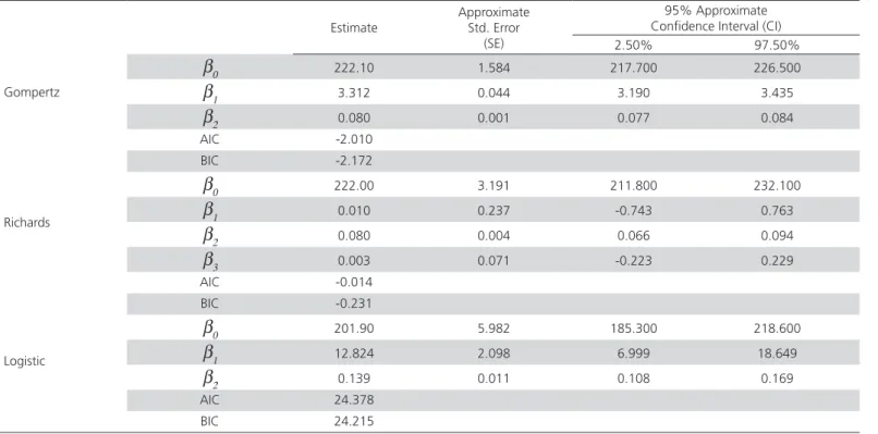
Parameter estimates, their approximate standard errors and 95% confidence intervals obtained from the classical approach (NLS) for the three growth functions are given in Table 1 for completeness. Also, Table 2 provides the summary statistics of Bayesian analysis for the fitted functions.

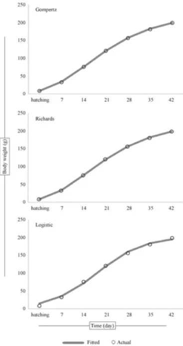
Gompertz function has the best fit to the data in terms of model selection criteria, AIC and BIC, followed by Richards and Logistic functions using classical approach, NLS. On the other hand, Figure 1 depicts the fit of three growth functions to the actual values within Bayesian context. From the figure, it can clearly be seen that all models are accurate in prediction of the actual body weights. The DIC statistics of the aforementioned models indicated that both the Gompertz and Richards functions fits the data exactly the same and also are better than the logistic function (Table 2). Comparing the goodness of fit of various growth functions to quail data, numerous studies have shown that Gompertz and Richards functions reflect the age-weight relationship of Japanese quails well (Tzeng & Becker, 1981; Anthony et al., 1991; Akbas & Oguz, 1998; Mignon-Grasteau et al., 1999; Sezer &Tarhan, 2005; Alkan et al., 2009; Narinc et al., 2010).

Similar parameter estimates were obtained when classical and Bayesian approaches were considered (Tables 1 and 2). The standard deviations (SD) of the posterior distribution are analogous to the approximate standard error (SE) estimates of the parameters which can be produced by default in any statistical package. In this respect, SDs (Table 2) were used as equivalent estimates of the SEs (Table1). For the Gompertz function, the Bayesian analysis resulted higher SDs of the parameter estimates than their corresponding SEs. The Bayesian estimation of the Richards function produced smaller SDs for all the parameters. While the posterior SD of β₀ is higher than its SE in NLS estimation, smaller SEs are obtained for β₁ and β₂ when fitting the logistic function. In the Bayesian context, the classical confidence intervals (CI) are replaced by the Bayesian credible intervals (BCI). Both CI and BCI for the Gompertz function parameters were similar, while BCIs are narrower than CIs for Logistic and Richards function parameters (Tables 1 and 2). On the other hand, CIs of both β₁ and β₃ parameters of

Richards function include zero, and are considered to be statistically insignificant. Non-significance of any of the estimated parameters of a growth function might have several reasons (Fekedulegn et al., 1999): 1) one or more parameters in the function may not be useful, or model can be reparameterized to involve less parameters; 2) the growth data are not adequate to estimate all parameters in the function; or 3) the assumptions of the function do not conform with the biological system being modeled. Moreover, it was reported that convergence problems may occur in fitting Richards function (Darmani Kuhi et al., 2003; Karkach, 2006). Although Logistic function led to statistically significant parameter estimates using NLS approach,

as can be seen by a better fit of Richards function than the Logistic function, significant parameter estimates do not always guarantee a good fit to the data, and therefore this should not be the only criterion to select

the best fitting model for the data in hand (Darmani Kuhi et al., 2003). Contrary to NLS method, BCIs of the parameters in Richards function do not include zero. This is due to the power of Bayesian approach

Table 2 – Posterior summary statistics for the three growth functions

Median Mean SD MCError 95% Credible Interval (BCI)

2.50% 97.50%

Gompertz

β₀ 222.10 222.14 2.14 0.080 217.80 226.60

β₁ 3.312 3.312 0.057 0.002 3.195 3.429

β₂ 0.080 0.080 0.002 0.000 0.077 0.083

σ2 _{0.653 1.031 1.871 0.044 0.198 4.059}

DIC 22.3

Richards

β₀ 221.80 221.86 2.19 0.071 217.70 226.31

β₁ 0.014 0.015 0.003 0.000 0.012 0.021

β₂ 0.080 0.080 0.002 0.000 0.077 0.084

β₃ 0.004 0.005 0.001 0.000 0.004 0.007

σ2 _{0.646 1.077 1.772 0.047 0.200 4.766}

DIC 22.3

Logistic

β₀ 202.00 202.58 7.26 0.254 189.70 217.30

β₁ 12.630 12.586 1.341 0.186 9.491 14.940

β₂ 0.138 0.138 0.009 0.001 0.117 0.156

σ2 _{23.870 34.076 34.914 1.238 8.060 117.805}

DIC 46.9

SD: Standard deviation; MCError: Monte Carlo Error; DIC: Deviance information criterion Table 1 – NLS estimation results for the three growth functions

Estimate

Approximate Std. Error

(SE)

95% Approximate Confidence Interval (CI)

2.50% 97.50%

Gompertz

β₀ 222.10 1.584 217.700 226.500

β₁ 3.312 0.044 3.190 3.435

β₂ 0.080 0.001 0.077 0.084

AIC -2.010

BIC -2.172

Richards

β₀ 222.00 3.191 211.800 232.100

β₁ 0.010 0.237 -0.743 0.763

β₂ 0.080 0.004 0.066 0.094

β₃ 0.003 0.071 -0.223 0.229

AIC -0.014

BIC -0.231

Logistic

β₀ 201.90 5.982 185.300 218.600

β₁ 12.824 2.098 6.999 18.649

β₂ 0.139 0.011 0.108 0.169

AIC 24.378

BIC 24.215

in estimating the parameters of complex functions, particularly with small data sets.

Although the parameters of the functions are represented with the same letters, they do not have the same biological meaning, except the asymptotic weight parameter, β₀, and comparison of the parameter estimates across the models is not reasonable. The asymptotic weight parameter estimates obtained from fitting Gompertz, Richards and Logistic functions are 222.10, 221.80 and 202.00, respectively. These values of β₀ parameter are higher than Anthony et al. (1991) have reported. Similar results have been reported by Akbas & Oguz (1998), Kizilkaya et al. (2005) and Alkan et al. (2009). The differences in the parameter estimates of growth functions may occur among different studies as a result of having different genotype and environmental conditions.

Gompertz and Logistic functions have a priori

defined growth shapes with inflection point at 37% and 50% of the asymptote, respectively (Grimm & Ram, 2009). In the Richards function, an additional parameter, β₃, allows the flexibility in the inflection point. Moreover, the Gompertz and Logistic growth functions can be derived from the Richards function. When the β₃ parameter in Richards function approaches 0, Gompertz function is approximated, where as if

β₃ parameter approaches 1, the Logistic function is obtained (Sezer & Tarhan, 2005;Kizilkaya et al., 2006). When choosing an appropriate function to model growth in biological systems, researchers need to pick a model that is flexible with the least complexity among the available functions. For instance, the Gompertz and Logistic functions are simple and were shown to fit well to short time series such as growth data of animal species (Darmani Kuhi et al., 2010). Compared to Gompertz and Logistic functions, Richards function is more complex, has an additional parameter and can fit well to the complex patterns but it is difficult to fit and requires a long time series (Karkach, 2006).

CONCLUSIONS

In this paper, we considered the estimation of the growth curve parameters for nonlinear models using classical and Bayesian methods. Both classical and Bayesian methods of estimation are well established and it is not necessary to justify why one or the other is preferred (Blasco, 2001). The Bayesian methodology can be applied without restriction to the growth functions used in this study. However, Bayesian analyses are sensitive to the choice of priors and different priors

may result in different posterior expectations of the parameters. Since the parameters of the normal priors (hyper parameters) were chosen so as to yield nearly a flat distribution, classical and Bayesian estimates did not differ much for the nonlinear curve parameters. Further study may be carried out to examine the effects of different prior specifications in nonlinear functions and to estimate their parameters in Bayesian context. However, the Bayesian method consistently predicts narrower credible intervals and gives more accurate results than those from the classical approach. When using the Bayesian methodology, it is possible to proceed to the comparisons among these parameters without having to resort to asymptotic procedures and incoherent results through frequentist theories. It is also important to note that use of these procedures need not be confined to any specific class of models. Rather, they can be applied to a wide range of model determination problems.

ACKNOWLEDGEMENT

We would like to express our gratitude to Dr. Tulin Aksoy (Akdeniz University, Faculty of Agriculture, Department of Animal Science, Antalya-TURKEY) for supplying the data, which was collected as part of a research project supported by Akdeniz University Scientific Research Projects Management Unit (project number: 2005.02.0121.005).

REFERENCES

Aggrey SE. Comparison of three nonlinear and spline regression models for describing chicken growth curves. Poultry Science 2002;81:1782-1788.

Ahmadi H, Golian A. Non-linear hyperbolastic growth models for describing growth curve in classical strain of broiler chicken. Research Journal of Biological Sciences 2008;3(11):1300-1304.

Akbas Y, Oguz I. Growth curve parameters of lines of Japanese quail (Coturnix coturnix japonica), unselected and selected for four-week body weight. Archiv Fur Geflugelkunde 1998;62(3):104-109.

Alkan S, Mendes M, Karabag K, Balcioglu MS. Effect of short-term divergent selection for 5-week body weight on growth characteristics of Japanese quail. Archiv Fur Geflugelkunde 2009;73(2):124-131. Anthony NB, Emmerson DA, Nestor KE, Bacon WL. Comparison of growth

curves of weight selected populations of turkeys, quail and chickens. Poultry Science 1991;70:13-19.

Blasco A, Piles M, Varona L. A Bayesian analysis of the effect of selection for growth rate on growth curves in rabbits. Genetics Selection Evolution 2003;35:21-41.

Darmani Kuhi H, Kebreab E, Lopez S, France J. An evaluation for different growth functions for describing the profile of live weight with time (age) in meat and egg strains of chicken. Poultry Science 2003;82:1536-1543.

Darmani Kuhi H, Porter T, Lopez S, Kebreab E, Strathe AB, Dumas A, et al. A review of mathematical functions for the analysis of growth in poultry. World’s Poultry Science Journal 2010;66:227-239.

Emmans GC. Problems in modeling the growth of poultry. World’s Poultry Science Journal 1995;51:77-89.

Fekedulegn D, Mac Siurtain MP, Colbert JJ. Parameter Estimation of nonlinear growth models in forestry. Silva Fennica 1999;33(4):327-336. Firat MZ, Theobald CM, Thompson R. Multivariate analysis of test day milk

yields of British Holstein Friesian heifers using Gibbs sampling. Acta Agriculturae Scandinavica, Section A 1997b;47:221-229.

Firat MZ, Theobald CM, Thompson R. Univariate analysis of test day milk yields of British Holstein Friesian heifers using Gibbs sampling. Acta Agriculturae Scandinavica, Section A 1997a;47:213-220.

Firat MZ. Bayesian analysis of test day milk yields in an unbalanced mixed model assuming random herd-year-month effects. Turkish Journal of Veterinary and Animal Sciences 2001;25:327-333.

Forni S, Piles M, Blasco A, Varona L, Oliveira HN, Lobo RB, et al. Comparison of different non-linear functions to describe the Nelore cattle growth. Journal of Animal Science 2009;87:496-506.

Grimm KJ, Ram N. Nonlinear growth models in Mplus and SAS. Structural Equation Modeling 2009;16(4):676-701.

Karkach AS. Trajectories and models of individual growth. Demographic Research 2006;15:347-400.

Kizilkaya K, Balcioglu MS, Yolcu HI, Karabag K, Genc IH. Growth curve analysis using nonlinear mixed model in divergently selected Japanese quails. Archiv Fur Geflugelkunde 2006;70(4):181-186.

Kizilkaya K, Balcioglu MS, Yolcu HI, Karabag K. The application of exponential method in the analysis of growth curve for Japanese quail. Archiv Fur Geflugelkunde 2005;69(5):193-198.

Lunn D, Thomas A, Best N, Spiegelhalter DJ. Win BUGS - a Bayesian modeling framework: concepts, structure, and extensibility. Statistics and Computing 2000;10:325-337.

Marks HL. Growth curve changes associate with long term selection for body weight Japanese quail. Growth 1978;42:129-140.

Mignon-Grasteau S, Beaumont C, Rochambeau H, Poivey JP, Ricard FH. Genetic parameters of growth curve parameters in male and female chickens. British Poultry Science 1999;40:44-51.

Narinc D, Aksoy T, Karaman E, Karabag K. Effect of selection applied in the direction of high live weight on growth parameters in Japanese quails. Akdeniz Üniversitesi Ziraat Fakültesi Dergisi 2009;22(2):149-156. Narinc D, Karaman E, Firat MZ, Aksoy T. Comparison of non-linear growth

models to describe the growth in Japanese quail. Journal of Animal and Veterinary Advances 2010;9(14):1961-1966.

R Development Core Team. R: a language and environment for statistical computing, reference index version 2.12.1. Vienna; R Foundation for Statistical; 2010.

SAS Institute. SAS/STAT user’s guide. Version 9.2. Cary; 2009.

Sezer M, Tarhan S. Model parameters of growth curves of three meat-type lines of Japanese quail. Czech Journal of Animal Science 2005;50(1):22-30.

Spiegelhalter DJ, Best NG, Carlin BP, Van Der Linde A. Bayesian measures of model complexity and fit. Journal of the Royal Statistical Society, Series B 2002;64:583-640.

Spiegelhalter DJ, Thomas A, Best NG, Lunn D. WinBUGS user manual: Version 1.4. MRC Biostatistics Unit. Cambridge; 2003.

Theobald CM, Firat MZ, Thompson R. Gibbs sampling, adaptive rejection sampling and robustness to prior specification for a mixed linear model. Genetics Selection Evolution 1997;29:57-72.

Tzeng RY, Becker WA. Growth patterns body and abdominal fat weights in male broiler chickens. Poultry Science 1981;60:1101-1106.

Vuori K, Stranden I, Sevon-Aimonen ML, Mantysaari EA. Estimation of non-linear growth models by linearization: a simulation study using a Gompertz function. Genetics Selection Evolution 2006;38:343-358. Zhang Z, Hamagami F, Wang L, Nesselroade JR, Grimm KJ. Bayesian analysis