Methods to verify parameter equality in nonlinear
regression models
Lídia Raquel de Carvalho; Sheila Zambello de Pinho*; Martha Maria Mischan
UNESP/IB - Depto. de Bioestatística, C.P. 510 – 18618-970 – Botucatu, SP - Brasil. *Corresponding author <[email protected]>
ABSTRACT: In biologic experiments, in which growth curves are adjusted to sample data, treatments applied to the experimental material can affect the parameter estimates. In these cases the interest is to compare the growth functions, in order to distinguish treatments. Three methods that verify the equality of parameters in nonlinear regression models were compared: (i) developed by Carvalho in 1996, performing ANOVA on estimates of parameters of individual fits; (ii) suggested by Regazzi in 2003, using the likelihood ratio method; and (iii) constructing a pooled variance from individual variances. The parametric tests, F and Tukey, were employed when the parameter estimators were near to present the properties of linear model estimators, that is, unbiasedness, normal distribution and minimum variance. The first and second methods presented similar results, but the third method is simpler in calculations and uses all information contained in the original data. Key words: logistic model, treatments comparison
Métodos de verificação de igualdade de parâmetros em modelos
de regressão não-linear
RESUMO: Em experimentos biológicos, em que curvas assintóticas de crescimento são ajustadas a resultados amostrais, o padrão de crescimento pode ser afetado por tratamentos aplicados ao material experimental. Nesses casos há interesse em comparar as diferentes funções de crescimento, com o objetivo de diferenciar os tratamentos. Compararam-se três métodos de verificação de igualdade de parâmetros em modelos de regressão não-linear: (i) desenvolvido por Carvalho em 1996, o qual realiza análises de variância com estimativas dos parâmetros resultantes de ajustamentos do modelo em cada unidade experimental; (ii) sugerido por Regazzi em 2003, utilizando o método da razão da máxima verossimilhança; e (iii) construindo uma variância conjunta a partir das variâncias individuais das estimativas dos parâmetros obtidas nos ajustamentos do modelo. Os testes F e Tukey foram empregados quando foi possível considerar os estimadores dos parâmetros com propriedades próximas às dos estimadores de modelos lineares, isto é, não-tendenciosidade, distribuição normal e variância mínima. Os dois primeiros métodos apresentaram resultados semelhantes quanto à discriminação dos tratamentos; o terceiro método diferiu dos anteriores, mas tem a vantagem de apresentar simplicidade nos cálculos, além de utilizar toda a informação contida nos dados originais.
Palavras-chave:modelo logístico, comparação de tratamentos
Introduction
In biologic studies growth curves have many impor-tant applications and the description and comparison among them by regression models is an efficient quan-titative method. Linear and nonlinear functions have been adjusted to data in many studies involving experi-ments comprising several treatexperi-ments. In these cases the objective is to verify differences among treatments ac-cording to the adjusted curves.
To make these comparisons parametric methods have been employed in which growth curves are adjusted to each experimental unit to obtain parameter estimates and conduct an analysis of variance. In relation to non-linear regression models, Carvalho (1996) worked with logistic and Gompertz functions, Whyte and Woollons (1990) with Gompertz, Santos et al. (1999) used the Weibull model and comparing two groups utilizing t-test; with respect to linear models, among others, there is the work of Meredith and Stehman (1991), adjusting
polynomial models and comparing treatments. Treat-ment comparisons may be made through the Tukey-test, as in Carvalho (1996), or t-test as in Santos et al. (1999), or using a regression analysis for treatments as levels of a quantitative factor (Meredith and Stehman, 1991).
The objective of the present study was to compare some methods that verify if a certain parameter of a nonlinear re-gression presents constant values in two or more treatments.
Material and Methods
The logistic regression model: y = α [1-β exp(-γ x)]–1, with α, β and γ as parameters, was adjusted to the data of each treatment. In order to compare the effects of a treatment on the parameter estimates, three methods de-scribed below were employed.
Method 1 (m1): Carvalho (1996) presented a method for comparison of logistic and Gompertz parameters using parametric tests. As described in Bates and Watts (1988) an important requirement to establish confidence inter-vals and regions of parameters in nonlinear models, us-ing linear approximation, is that the expected surface in the parametric space should be flat so that the tangent plane would give a precise approximation. There are nonlinear relative curvature measures (C) that can be uti-lized to indicate if the linear approximate in a particu-lar case is adequate. Curvatures are considered little when their measures are smaller than the circle 95% con-fidence, that is, if C ≤ 1 / F or if C F ≤ 1, where F = F(P, N - P; 0.05), with P = number of parameters of the model and N = number of data pairs. An expected sur-face with radius 1/C is considered, and the deviation of the surface from the tangent plane at a distance F from the tangent point is determined. This deviation is ex-pressed as a percentage of the confidence radius of the circle, and is 100( 1−C F)/C F. If C ≤ 1 / F= 0.1, then the deviation from the surface is 5%, if C ≤ 1 / F= 0.2, the deviation is 10%, and if C ≤ 1 / F= 0.3, is 15%. Consequently, the analysis is adequate if the curvature C F is ≤ 0.3.
In the present study the logistic function was adjusted to each experimental unit, and the Bates and Watts cur-vature measures, that is, the intrinsic nonlinearity and the parameter-effect nonlinearity, were calculated. When the measures were below 0.3, and the basic as-sumptions of the analysis of variance were satisfied, each model parameter was analyzed; afterwards the differ-ences between treatments were verified by the Tukey method. Because the logistic was adjusted to each experi-mental unit there were 16 fitted functions, each with ten pairs {x,y} and, therefore, seven degrees of freedom (df) for the mean square error. The analysis of variance of the resulting estimated parameters had therefore 16 val-ues classified as eight treatments and two replicates; here there were eight df for the mean square error.
Method 2 (m2): Regazzi (1993) considered the adjustment of H polynomial regression equations of degree k, em-ploying orthogonal polynomials techniques. He pre-sented, in detail, a method to test the following hypoth-eses: (a) H0: the H equations are identical; (b) H0: the H equations have a common regression constant; (c) H0: the H equations have one or more equal regression co-efficients. This author concluded by the generality of the method, and that it can be used in polynomial models of any degree, orthogonal or not, and also in multiple regression models. Regazzi (2003) considered the adjust-ment of g nonlinear regression equations (g groups), with the objective to present an adequate methodology to test
the following hypotheses, employing the likelihood ra-tio test: (a) H0: the g equations are identical, that is, a common equation can be used as an estimate of the g considered equations; and (b) H0: a determined subset of parameters is equal.
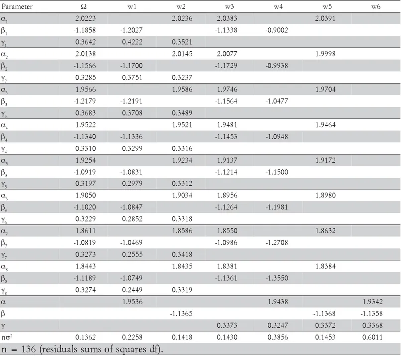
The following models were adjusted: Ω = unre-stricted model, where the three parameters are adjusted to each treatment; w1 = restricted model, where the α parameter is common to all treatments; this model is verified by the hypothesis H0(1); w2 = restricted model, where the β parameter is common to all treatments; this model is verified by the hypothesis H0(2); w3 = restricted model, where the γ parameter is common to all treat-ments; this model is verified by the hypothesis H0(3); w4 = restricted model, where the α and γ parameters are common to all treatments; this model is verified by the hypothesis H0(4); w5 = restricted model, where the β and γ parameters are common to all treatments; this model is verified by the hypothesis H0(5); w6 = restricted model, with all parameters common to all treatments; this model is verified by the hypothesis H0(6). These hy-potheses are mathematically described in Table 2.
Method 3 (m3): The nonlinear regression model was ad-justed to each treatment and the parameter estimates θi, i = 1,..., P, P = 3, their asymptotic variances and their direct measures of skewness of Hougaard (1985), g1i, were obtained. With ten time points and two replicates there were 20 pairs {x,y}, therefore with 17 df for the mean square error. As a result of the logistic fitting there were eight estimated parameters and corresponding estimated variances. The comparison between two α-estimates L =αˆi - αˆj , i, j = 1,...,8, i ≠ j, is then considered.
A description of the Hougaard method to obtain these measures of skewness can be found in Ratkowsky (1989); this author classified the measures as follows: if |g1i|< 0.1, the estimator θˆiof parameter θi has a very
close-to-linear behavior; if 0.1 < |g1i| < 0.25, the esti-mator is reasonably close-to-linear; if |g1i| ≥ 0.25, the skewness is very apparent; and if |g1i| >1 this indicates a considerable nonlinear behavior. This terminology, ‘close-to-linear’, according to Ratkowsky (1989), refers to nonlinear regression models with estimators near to present the properties of linear models estimators, that is, unbiasedness, normal distribution and minimum vari-ance. Consequently, considering the adjustments with low Hougaard measures, the parameter estimates were compared through the Tukey test, using the estimates of their variances.
Results and Discussion
Method 1 - The measures of intrinsic nonlinearity and
effects on α-estimates, with the value of 0.0421 as a test criterion (q = 5.596).
Method 2 - The results of the adjusted models are
pre-sented in Tables 1 to 3.
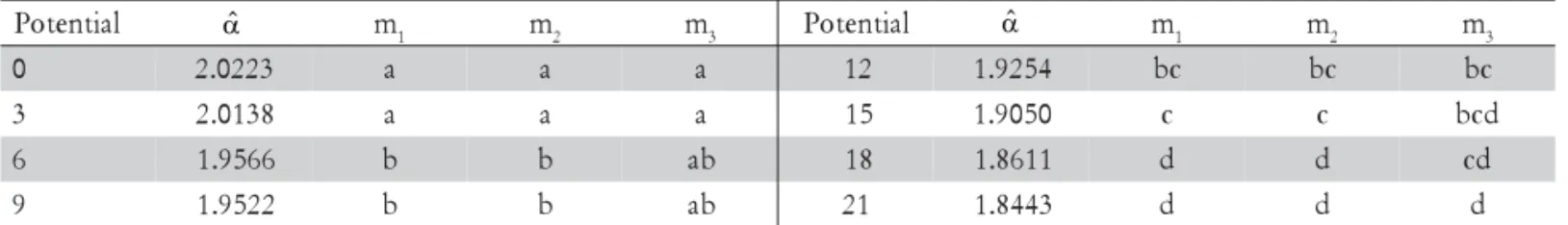
Method 3 - The logistic model adjusted to each
treat-ment data resulted in the estimates of the α parameter presented in Table 4. The g1 values are all near 0.1, there-fore the models were considered as close-to-linear mod-els. The eight variance estimates of α-estimates may be considered homogeneous in accordance to the Bartlett test, with χ2 = 2.75, 7 df, then an average variance was
r e t e m a r a
P Ω w1 w2 w3 w4 w5 w6
α1 2.0223 2.0236 2.0383 2.0391
β1 -1.1858 -1.2027 -1.1338 -0.9002
γ1 0.3642 0.4222 0.3521
α2 2.0138 2.0145 2.0077 1.9998
β2 -1.1566 -1.1700 -1.1729 -0.9938
γ2 0.3285 0.3751 0.3237
α3 1.9566 1.9586 1.9746 1.9704
β3 -1.2179 -1.2191 -1.1564 -1.0477
γ3 0.3683 0.3708 0.3489
α4 1.9522 1.9521 1.9481 1.9464
β4 -1.1340 -1.1336 -1.1453 -1.0948
γ4 0.3310 0.3299 0.3316
α5 1.9254 1.9234 1.9137 1.9172
β5 -1.0919 -1.0831 -1.1214 -1.1500
γ5 0.3197 0.2979 0.3312
α6 1.9050 1.9034 1.8956 1.8980
β6 -1.1020 -1.0847 -1.1264 -1.1981
γ6 0.3229 0.2852 0.3318
α7 1.8611 1.8586 1.8550 1.8632
β7 -1.0819 -1.0469 -1.0986 -1.2708
γ7 0.3273 0.2555 0.3418
α8 1.8443 1.8435 1.8381 1.8384
β8 -1.1189 -1.0749 -1.1361 -1.3550
γ8 0.3274 0.2449 0.3319
α 1.9536 1.9438 1.9342
β -1.1365 -1.1368 -1.1358
γ 0.3373 0.3247 0.3372 0.3368
nσ2 0.1362 0.2258 0.1418 0.1430 0.3856 0.1453 0.6011
.
)
f
d
s
e
r
a
u
q
s
f
o
s
m
u
s
s
l
a
u
d
i
s
e
r
(
6
3
1
=
n
Table 1 - Parameter estimates of the unrestricted model (Ω) and restricted models (w1 to w6), and the correspondent
residuals sums of squares.
Table 2 - Hypotheses under consideration.
H0(1):α1=α2=α3=α4=α5=α6=α7=α8=α
H0(2):β1=β2=β3=β4=β5=β6=β7=β8=β
H0(3):γ1=γ2=γ3=γ4=γ5=γ6=γ7=γ8=γ
H0(4):α1=α2=α3=α4=α5=α6=α7=α8=αandγ1=γ2=γ3=γ4=γ5=γ6=γ7=γ8=γ
H0(5):β1=β2=β3=β4=β5=β6=β7=β8=βandγ1=γ2=γ3=γ4=γ5=γ6=γ7=γ8=γ
calculated, s2 = 0.000297, with 136 df. This estimated variance can be used in tests, as Tukey test to compare different α-estimates; the calculated Tukey minimum significant difference was 0.0750 (q = 4.352). See Table 5 that includes also the results of the other two meth-ods.
The conclusions about differences among treatment effects were the same for methods 1 and 2. The differ-ent conclusions between methods 1 and 3 may be attrib-uted to different errors used as a base for the tests. With method 1 a regression analysis was performed on each experimental unit, then a data set of ten values was used, with seven df in error; from these analyses, 16 estimates of α-parameter are obtained, that were submitted to the analysis of variance with eight treatments and two rep-lications, and an error degree of freedom of 8 is obtained. These α-estimates, however, have already a variance with seven df for method 1 and 20-3 = 17 df for method 3, because the latter uses a data set with 20 pairs to per-form a single regression per treatment. This additional information is used by method 3 in order to obtain the average variance with 136 df.
The estimated average variance employed by method 3 is also a base to verify the significance of a simple lin-ear regression model relating the α-estimates and the po-tential (treatment) values; this is more appropriate than the Tukey test before performed, because the treatments are quantitative level factors. The estimated regression equation is
α
=2.0264–0.00869*po, with po = potential values, a 5% significant model, with determination
co-efficient R2 = 0.976. Figure 1 represents the regression model.
Conclusions
Method 1 (Carvalho, 1996) and method 2 (Regazzi, 2003) presented similar results; however method 3 had less significant differences. Nevertheless, method 3 is simpler in calculations and uses all information con-tained in the original data.
Acknowledgements
To the program “CAPES Pró-Equipamentos no 1, 01/ 2007” by the equipments provided.
l a i t n e t o
P m
1 m2 m3 Potential m1 m2 m3
0 2.0223 a a a 12 1.9254 bc bc bc
3 2.0138 a a a 15 1.9050 c c bcd
6 1.9566 b b ab 18 1.8611 d d cd
9 1.9522 b b ab 21 1.8443 d d d
Table 5 - Estimates of α-parameter obtained through the logistic function adjusted to data of the example. Comparisons
among the estimates by the Tukey test (5% level of significance), performed with the three methods (m1, m2,
m3).
αˆ αˆ
H0 χ2cal df p-value H0 χ2cal df p-value
1 80.88 1 2.39E-19 4 166.51 2 6.97E-37
2 6.45 1 0.011115 5 10.34 2 0.015827
3 7.80 1 0.005238 6 237.54 3 3.24E-51
Table 3 - Chi-square values (χ2 cal) with the associated degrees of freedom (df), and p-value of the test.
) o p ( l a i t n e t o
P var(17df) g1 Potential(po) var(17df) g1
0 2.0223 0.000390 0.12 12 1.9254 0.000316 0.14
3 2.0138 0.000273 0.12 15 1.9050 0.000386 0.15
6 1.9566 0.000265 0.10 18 1.8611 0.000198 0.11
9 1.9522 0.000267 0.12 21 1.8443 0.000283 0.13
Table 4 - Estimates of α-parameter, variances, and the Hougaard measures of skewness (g1).
αˆ αˆ
Figure 1 - Linear decreasing regression model between α -estimates (αˆ ) of the logistic function and potential values (po).
1.80 1.85 1.90 1.95 2.00 2.05
0 3 6 9 12 15 18 21
po
References
Bates, D.M.; Watts, D.G. 1988. Nonlinear regression analysis and its applications. John Wiley, New York, NY, USA. 365p. Carvalho, L.R. Métodos para comparação de curvas de crescimento.
1996. Dr. Thesis. UNESP/FCA, Botucatu, SP. Brazil. (In Portuguese, with Summary in English).
Hougaard, P. 1985. The Appropriateness of the asymptotic distribution in a nonlinear regression model in relation to curvature. Journal of the Royal Statistical Society, Serie B 47: 103-114.
Meredith, M.P.; Stehman, S.V. 1991. Repeated measures experiments in forestry: focus on analysis of response curves. Canadian Journal of Forest Research 21: 957-965
Ratkowsky, D.A. 1989. Handbook of Nonlinear Regression Models. Marcel Dekker, New York, NY, USA. 241p.
Regazzi, A.J. 1993. Teste para verificar a identidade de modelos de regressão e a igualdade de alguns parâmetros num modelo polinomial ortogonal. Revista Ceres 40: 176-195.
Regazzi, A.J. 2003. Teste para verificar a igualdade de parâmetros e a identidade de modelos de regressão não-linear. In: Reunião da RBRAS 48. Lavras, MG, Brazil.
Santos, S.A.; Souza, G.S.; Oliveira, M.R.; Sereno, J.R.B. 1999. Using nonlinear models to describe height growth curves in Pantaneiro horses. Pesquisa Agropecuária Brasileira 34: 1133-1138. Whyte, A.G.D.; Woollons, R.C. 1990. Modeling stand growth of
radiata pine thinned to varying densities. Canadian Journal of Forest Research 20: 1069-1076.