Experimental study of a similarity metric for retrieving pieces from structured plan cases: its role in the originality of plan case solutions

Experimental Study of a Similarity Metric for

Retrieving Pieces from Structured Plan Cases: its Role in

the Originality of Plan Case Solutions

) Instituto Superior de Engenharia de Coimbra, 3030 Coimbra, Portugal ([email protected])

(2

) CISUC - Centro de Informática e Sistemas da Universidade de Coimbra, Polo II, 3030 Coimbra, Portugal

([email protected], [email protected], [email protected])

A b s t r a c t . This paper describes a quantitative similarity metric and its

contribution to achieve original plan solutions. This similarity metric is used by an iterative process of piece retrieval from structured plan cases. Within our approach plan cases are tree-like networks of pieces (goals and actions). These case pieces are ill-related each other by links (explanations). These links may be classified as hierarchical or temporal, antecedent or consequent, and explicit or implicit. Besides links, each case piece has also information about its properties (the attributes-value pairs), its hierarchical and temporal position in the case (the address), and about its constraints in the relationship with others (the constraints). The similarity metric computes a similarity value between two case pieces taking into account similarities between these case piece’s information types. Each time a problem is proposed, different weights are given to some of those similarities, with the aim of solving it with an original solution. This similarity metric is used by the system INSPIRER (ImagiNation taking as Source Past and Imperfectly REalated Reasonings). We illustrate the role of the similarity metric in the creativity of solutions, focusing specially their originality, with the presentation of the experimental results obtained in the musical composition domain, which is considered by us as a planning domain.

1 Introduction

The power of a Case-Based Reasoning (CBR) System (Kolodner and Riesbeck, 1986) is greatly determined by its capability to retrieve the relevant cases for the solution of a new problem. A nearest neighbour algorithm for case retrieval (Duda and Hart, 1973) searches through every case in memory, applies a similarity metric and returns the case or k cases with the past problem more similar to the new one. This similarity metric counts the number of facts that the past and the new problem have in common. Knowledge-based retrieval systems (Koton, 1989) are a consequence of combining nearest neighbour and knowledge-guided techniques. These systems are characterised by the use of domain knowledge for the construction of explanations for why a problem had a particular solution in the past. Those explanations are necessary to similarity judgement (Barletta and Mark, 1989; Veloso, 1992; Bento and Costa, 1994): they are necessary to judge the relevance of the features comprising a past problem. In domains

where a strong theory is not available but past experience is accessible, case explanations are imperfect (Bento, Macedo and Costa, 1994). CBR is appropriate for this kind of domains.

Although many CBR systems select out cases that are most similar to the new problem, other selection criteria may prove more effective. E.g., Kolodner (1989) has considered that the most useful cases are those that can address the reasoner’s current goal, which means that they may not be the most similar ones. Particularly, this stands to reason when the goal is to achieve creative solutions, i.e., solutions required to be original but also appropriate (Macedo et al. 1996b, 1996c 1997a).

Considering cases as set of pieces (Barletta and Mark, 1988; Kolodner, 1988; Redmond, 1990; Sycara and Navinchandra, 1991; Veloso, 1992; Bento, Macedo and Costa, 1994) instead of monolithic entities, can improve the results of a CBR system in that solutions of problems may result from the contribution of multiple cases.

Moreover, structured representations of cases (Plaza, 1995) allow treating pieces of cases as full-fledged cases. This has two consequences: first, the similarity metric used by the nearest neighbour algorithm can be applied to them; second, the problems that appear when using parts of multiple monolithic cases are minimised, particularly, the lot of effort taken to find the useful parts in them.

A plan is a specific sequence of steps (or actions) with the aim of a goal achievement. Case-Based Planning (CBP) systems (Hammond, 1986; Veloso, 1992) reuse past sequences of actions from past plans to construct new ones. Some systems like CELIA (Redmond, 1990), JULIA (Kolodner, 1989), PRODIGY/ANALOGY (Veloso, 1992), etc., break up the goal into smaller sub-goals, enabling plan construction by composition of sub-plans. This leads to a hierarchical representation of plan cases (Macedo et al., 1996a). The case representation is similar to a tree where each node is a goal and its sons the sub-goals, or at the latest level, the actions of the plan. Each goal (or action) depends on other goals. This is particularly evident in structured domains.

In this paper we will focus on a similarity metric used by an iterative retrieval of case pieces from structured plan cases. This means that building a new plan case solution consists in an incremental association of case pieces, each one of these resulting from a retrieval process, which involves the application of a similarity metric to each candidate case piece present in memory. This means case pieces are treated as full-fledged cases. The similarity metric takes into account the address, context and attribute similarities between two case pieces. We propose a way to produce creative solutions, i.e., original but also appropriate solutions, based on applying the similarity metric giving different weights to its components, each time a problem is solved.

Our approach to case representation is presented in the next section. The retrieval and solution construction process are briefly presented in section 3. In section 4, we introduce the similarity metric. Section 5 focus the definition of creative solutions, and section 6 presents an application in the musical composition domain. The results obtained with our similarity metric function in this domain are presented in section 7. Finally, a conclusion about our work is made in section 8.

2 Case Representation

Within our approach a plan case is a set of goals and actions organised in a hierarchical way (Figure 1): a main goal (the main problem) is refined into sub-goals (the sub-problems), and so on, until reaching the actions (the leaf nodes of the tree) that satisfy the goals. It is worth noting that, although the actions are represented by the leaf nodes, some of their properties (attributes) are inherited from the attributes of their hierarchical ascendants.

Temporal Links g1 g22 g21 g13 g2 g3 g g11 g12 g31 g32 α λ β ψ π Hierarchical Links a112 a113

a111 a114 a211 a212

. . . .

. . .

. . . .

Figure 1 - Case structure. The g_i’s represent the goals and the a_i’s the actions.

In our model, each node of the hierarchical structure corresponds to a case piece. To complete the case structure, there are links between case pieces, representing causal justifications, or explanations. Some of these links maintain the hierarchical case structure, others reflect causal temporal relations between case pieces. Thus the existence of a case piece in a plan case is causally explained by several case pieces of the same plan case.

Considering the hierarchical links only (represented in Figure 1 by continuous arrows), the inherent meaning of the represented structure is: g, the main goal of the plan (or the main problem), is achieved by sequentially achieving sub-goals (sub-problems) g1, g2 and g3. Each one of these sub-goals is also broken up into other sub-goals. For example, g1 is broken up into g11, g12 and g13, and g2 into g21 and g22. To achieve the goal g11 the actions a111, a112, a113 and a114 must be sequentially executed by this temporal order.

Besides being explained by the goal-refinement process, through hierarchical links, a case piece may also be explained through temporal links (represented in Figure 1 by discontinuous arrows). For example, g21 (sub-goal of g2) is a consequence of case pieces g11 and g12, which is represented by the temporal links labelled α and _ , respectively.

A case piece has seven types of information describing its relevant aspects: a name that uniquely identifies the case piece, the name of the case to which the case piece belongs, the case piece address, the constraints, a set of attribute/value pairs, the antecedents and the consequents.

The address of a case piece in level n is represented by Nn:Nn-1:...:N0, where each

N_i  ⊄₀ (from now on we will call offsets to the Ni’s ). An offset L=Ni, 0 _ i < n,

means that the case piece with that address has a predecessor in level i of the tree which is the L-th son of its father (with the exception of the case piece in level 0, which has no ascendants and so its offset is always 0). The offset J=Nn means that

this case piece is the J-th son of its closer ascendant. Every case piece propagates its address to its descendants, that is, if the case piece’s address is Nn:...:N0, its M-th

son’s address will be M:Nn:...:N0. This representation embeds in its syntax,

explicitly, the position that a case piece and its ascendants occupy in the tree relatively to the others, and, implicitly, the hierarchical level that the case piece occupies in the tree.

Another information in a case piece is a set of attribute/value pairs describing several properties which characterise the case piece.

The constraints are also attribute/value pairs. The semantic of a set of constraints C = {a1 = vc1, a2 = vc2, ...,an = vcn} of a case piece p is: if p ascendants have any of the attributes a1,a2, ...,an, then its values must not be different from, respectively, vc1, vc2, ...,vcn; otherwise, p is incoherent with its ascendants. Thus constraints play the role of determining whether or not the case piece is a candidate to occupy a missing piece (see below) in a solution, depending on whether or not they are coherent with the attributes of the missing piece’s hierarchical ascendants.

Antecedents and consequents are causal links that follow, respectively, from and to other case pieces. Antecedent links show how a case piece is explained by the existence of other case pieces (e.g. in Figure 1, g21 is explained by g11 and g12 through the links labelled _ and _ , respectively, and by g2 through a father link). Consequent links show how a case piece explains the existence of other case pieces (e.g., in Figure 1, g21 partially explains g22 and g32 through links _ and _ , respectively, and a211 and a212 through father links).

Each antecedent or consequent link is classified into another two main kinds of links: hierarchical and temporal ones (described above).

Sometimes the type of relation between antecedent fact(s) and the consequent one may be unknown. This lack of a complete theory is common in CBR (Bento, Macedo and Costa, 1994). This idea leads to another classification of the links between case pieces: we say that a link between the case pieces a and b is explicit if we know it well and so we are able to represent it, and implicit if we can’t represent it because we do not know it well, although we know it exists. In Figure 1, g13 implicitly explains g21. There is not a concrete link between them, but it is coherent to assume that the existence of g21 is partially due to the previous occurrence of g13. We may also say that g implicitly explains g21, although there is not a well known relation between them.

We call the case piece context to the set of case pieces that surround it. We distinguish eight types of contexts according to the kind of link existing between the case piece considered and the surrounding ones. Thus, each one of these surrounding case pieces is included in one of the contexts of the set C = {antecedent-hierarchical-implicit context, antecedent-hierarchical-explicit context, antecedent-temporal-{antecedent-hierarchical-implicit context, antecedent-temporal-explicit context, consequent-hierarchical-implicit context, consequent-hierarchical-explicit context, consequent-temporal-implicit context or consequent-temporal-explicit context}. Notice that the name of the context reflects the classification of the link to the case piece. For example, in Figure 1, the contexts of g21 are: antecedent-hierarchical-implicit context = {g}; antecedent-hierarchical-explicit context = {g2}; implicit context = {g13};

antecedent-temporal-explicit context = {g11, g12}; consequent-hierarchical-implicit context = {}; consequent-hierarchical-explicit context = {a211, a212}; consequent-temporal-implicit context = {g31}; consequent-temporal-explicit context = {g22, g32}.

Since there is not any direct link between implicitly related case pieces, it is necessary to define a frontier to limit the number of case pieces of the implicit contexts. We assume that this frontier involves the nearest case pieces.

3 Overview of the Retrieval Process and Solution Construction

The construction of an entire solution is performed by an iterative retrieval of case pieces from memory to fill the missing ones in the tree-like partially complete solution. This process is made level by level starting at the highest hierarchical level and ending at the lowest hierarchical level, and in each level, starting from the leftmost to the rightmost case piece.

The process of retrieving a case piece from memory is the following. Consider that π is the structured solution currently being constructed, and π_{i a place on solution} π in which a case piece is missing. The retrieval of a case piece to be placed in π_i involves the following steps:

(i) construction of the set of candidate case pieces by selecting those which belong to the same level of π_i;

(ii) application of a constraint based filter to the case pieces selected in (i), eliminating those which constraints are incompatible with the attributes of the π_i’s ascendants. This step is performed as follows. Given a case piece p presented in memory, candidate to fill π_{i, and given the set of constraints Lc = {c1 = vc1, c2 =} vc2, ...,cn = vcn} of case piece p, and the union of the sets of attribute-value pairs La = {a1 = va1, a2 = va2, ...,am = vam} of the hierarchical ascendants of πi, then p is not filtered from the set of candidate case pieces to fill π_{i if and only if:} _ i _ {1,2,...,n}, ∀j _ {1,2,...,m}, _ _{aj= vaj} _ _La, _ _ _{ci= vci} _ _{Lc : ci = aj} _ _vci _ _vaj

(iii) application of a similarity metric (function CasePieceSim presented below) to each candidate case piece;

(iv) ranking of the candidates case pieces by their similarity metric value; (v) selection of the case piece with the highest similarity metric value;

(vi) validation of placing the selected case piece on π_{i. This step comprises the} verification of link incompatibilities between the selected case piece and the partially constructed solution for the given problem. Performing one of the following options solves these incompatibilities: (i) relaxing incompatibilities; (ii) selecting another case piece.

4 The Similarity Metric

The similarity metric computes similarities between two case pieces p and p’ and is described as follows:

CasePieceSim p p( , ' )= ↔AttrSim p p( , ' )+ ↔AddrSim p p( , ' )+ ↔ContSim p p( , ' ) + +

α φ λ

α φ λ

where ContSim, AttrSim and AddrSim are the functions that compute, respectively, the context, attribute and address similarities between p and p', as presented below, and α , _ and _ are the user assigned parameters that represent the weights given to

those similarities, respectively. AddrSim is the following:

AddrSim p p( , ') = ↔AbsASim p( ad, 'pad)+ ↔AdYOSim p( ad, 'pad)+ ↔AdSESim p( ad, 'pad)

+ +

φ φ φ

φ φ φ

1 2 3

1 2 3

where: AbsAdSim calculates the similarity between the addresses pad and p’ad,

respectively, of case piece p and p’; AdYOSim calculates the similarities between the component of the same addresses that contains the information about case pieces positions relatively to their old and young brothers; AdSESim calculates the similarities of the case pieces address relatively to the start and end of the case. The parameters _ 1, _ 2, and _ 3 represent the weights given to those similarities, respectively. These functions are presented as follows.

AbsAdSim is: AbsAdSim p p p p p p ad ad ad ad ad ad ( , ' ) ' ' = = ? 1 0 AdYOSim is: AdYOSim H R H R H NSons R H NSons R ( : , ' : ' ) ( ) ' ( ' ) = − − ↵ √ 1

This function compares the mappings into the interval (0,1) of the positions of each case piece relatively to its young and old brother. This mapping is done dividing the first offset of the case piece’s address (H or H’) by the number of sons of its father, whose value is given by the function NSons. Remember that the first offset H of the case piece’s address H:R tells us that the case piece is the Hth

son of its father, whose address is R. AdSESim is: AdSESim H R H R H Ha H R NPiecesLevel H R H Ha H R NPiecesLevel H R ( : , ' : ' ) ( : ) ( : ) ' ( ' : ' ) ( ' : ' ) = − + − + ↵ √ 1

This function is similar to the previous one. However, the mapping is done by first, summing the first offset of the case piece’s address and the number of case pieces of the same level that are younger than it (this value is computed by the function Ha), and then, dividing this sum value by the number of case pieces of the same level of that case piece (this value is given by the function NPiecesLevel).

AttrSim is defined as follows:

AttrSim p p Length p p Length p Length p a a a a ( , ' ) ( ' ) ( ) ( ' ) = ↔ + 2

where pa, p’a are the sets of attributes of, respectively, p and p’, and Length is the

function that computes the length of a set.

ContSim p p F p p i i i i i ( , ') ( , ') = ↔ = = λ λ 1 8 1 8

where each Fi is a function that computes similarities between two same types of

contexts of two case pieces, as described below. Each _ i is the weight given to each one of those similarities. The Fi functions is:

F p p

Length p p

Length p Length p SeqSim p p

i c c c c c c i i i i i i ( , ') ( ' ) ( ) ( ' ) ( , ' ) = ↔ + + 2 2 where ci is the i th

element of the set of contexts C (described above), and, pci and

p’ci are the ci contexts of p and p’, respectively. SeqSim is the function that computes

the similarity between sequences of elements in both lists.

5 Creative Solutions

Creative solutions are undoubtedly mainly characterised by two properties: appropriateness and originality.

An appropriate solution is one that fulfills the goal(s) of the problem, i.e., that is useful by satisfying a need. A solution, to be appropriate, should also be coherent, without incompatibilities between its components, and also able to be executed (Macedo et al., 1996b, 1996c, 1997a).

An original solution is one that is different from previous ones, i.e., is one that stands apart from the solutions that the individual or other people has already produced. It is singular, novel and somehow unpredictable.

Originality of solutions is measured comparing the solution with the past solutions stored in memory. This comparison is made piece by piece, computing the number of new relations that a case piece has in the new solution in comparison with the relations it has in old solutions. Appropriateness is measured by experts taking into account the coherence and usefulness of solutions.

6 Musical Composition Domain

Balaban (1992) and others, state that any music can be represented by a hierarchy of temporal objects (objects with an associated temporal duration), in such a way that each one has, as descendants, a sequence of sub-objects that starts and ends at the same start and ending point as the object’s. Figure 2 shows an example.

There are temporal causal relations in music (represented in Figure 2 by discontinuous arrows), since many musical objects may be causally explained, for instance, by transformations of some other object (e.g., repetition, variation, inversion, transposition, etc.). For example, in Figure 2, the temporal link between theme of Part1 and var1 of Part2 may represent a variation transformation which, when applied to theme originates var1. These temporal relations are represented in the antecedents and consequents informations fields of a case piece.

. . . . Part1 var2 var1 codetta Part2 Part3 Sonata

intro theme var2 codetta

ω τ τ ι theme ρ ρ D A E B E E α ρ α ρ

Figure 2 - A case in the music domain.

Each musical object has several properties which are represented in our approach by attribute/value pairs (e.g., {ton='I', meas=2/4} meaning that the tonality is 'I' and the measure is binary).

Additionally, each musical object has also a set of constraints, which are conditions that must be consistent with the attributes of its ascendants, when it is added to the new case (e.g., if a case piece has the set of constraints a = {meas=2/4, ton='II', etc} then it must not be a descendant of a case piece with tonality 'I', for instance). Thus the role of the constraints is to maintain the coherence of the new musical piece hierarchy, since they disallow the hierarchical association of case pieces with incompatible properties.

The goal of our application is to use analysis of music pieces from a seventeenth century composer as foundation for a restructuring process, providing a structured and constrained way of composing novel pieces, although keeping the essential traits of the composer’s style. We use analysis of music pieces with six hierarchical levels. Each music piece is considered as a plan, since it is a sequence of musical objects with the aim of achieving a musical goal (e.g., a sonata).

7 Experimental Tests

7.1 Description and Results

The main aim of the tests performed with the similarity metric of INSPIRER in the musical composition domain is to evaluate its contribution to achieve original solutions. However, appropriateness is also guaranteed to a certain extent by the similarity metric since it disallows totally new solutions which may be inappropriate. Besides this, the tests also allow the formulation of conclusions about the accuracy of the INSPIRER's similarity metric.

We have made four tests (labelled Test #1, Test #2, Test #3 and Test #4) (Figure 3). In each test the values 0 or 1 were assigned to each parameter in the similarity metric function. In Test #1 the similarity metric is complete: it takes into account the attribute, address and context similarities (their parameters are assigned to 1). Test #2, #3 and #4 are similar to Test #1, with the difference of not taking into account, respectively, the context, the address and the attribute similarities in the similarity metric.

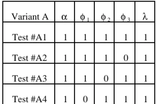
Test #1 has two variants: variant A (Figure 4) and variant B (Figure 5). Variant A corresponds to assigning different values (0 or 1) to the parameters of the sub-terms of

the similarity metric address term. Variant B is similar to variant A, but relatively to the sub-terms of the context term of the similarity metric.

Figure 5 - Test parameters for variant B of Test #1.

Each one of the Tests #2, #3, and #4, when compared with Test #1, allows to make conclusions about taking or not taking into account one term of the similarity metric. The same happen when comparing Tests #A2, #A3 and #A4 with Test #A1, and, Tests #B2, #B3,...,#B9 with Test #B1. This is based on the assumption that the best way to measure the relevance of xk to y, when y=f(x1,..., xk-1,, xk, xk+1,,..., xn), is

by comparing y1=f(x1,..., xk-1, xk+1,,..., xn) with y=f(x1,..., xk-1, xk, xk+1,,..., xn).

Some test conditions were kept constant in all the tests: we used just one past case solution in memory (a musical symphony), because we want to test the performance of INSPIRER's similarity metric in the worst conditions to achieve original solutions; the problem proposed was always the same: to produce a new symphony;

Variant A α φ1 φ2 φ3 λ Test #A1 1 1 1 1 1 Test #A2 1 1 1 0 1 Test #A3 1 1 0 1 1 Test #A4 1 0 1 1 1 α φ λ Test #1 1 1 1 Test #2 1 1 0 Test #3 1 0 1 Test #4 0 1 1

Figure 3 - Test parameters. Figure 4 - Test parameters for variant A of Test #1.

Variant B α φ λ1 λ2 λ3 λ4 λ5 λ6 λ7 λ8 Test #B1 1 1 1 1 1 1 1 1 1 1 Test #B2 1 1 1 1 1 1 1 1 1 0 Test #B3 1 1 1 1 1 1 1 1 0 1 Test #B4 1 1 1 1 1 1 1 0 1 1 Test #B5 1 1 1 1 1 1 0 1 1 1 Test #B6 1 1 1 1 1 0 1 1 1 1 Test #B7 1 1 1 1 0 1 1 1 1 1 Test #B8 1 1 1 0 1 1 1 1 1 1 Test #B9 1 1 0 1 1 1 1 1 1 1

each test produced a new case solution (a new symphony), which was evaluated by three musical composition teachers of the Coimbra School of Music, about its appropriateness and originality, taking as reference the original composer’s music piece, to which was given 100% of appropriateness.

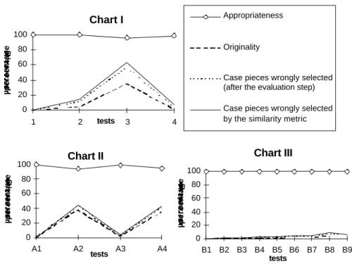
Chart I of Figure 6 summarises the results obtained with the four tests. Chart II shows the results of variant A of Test #1, and Chart III, the results of variant B of Test #1. Chart I 0 20 40 60 80 100 1 2 tests 3 4 percentage Appropriateness Originality

Case pieces wrongly selected (after the evaluation step) Case pieces wrongly selected by the similarity metric

Figure 6 - Test results. 7 . 2 A n a l y s i s o f R e s u l t s

From Chart I (Figure 6) we may conclude that the address term is the most important one to the accuracy of the similarity metric. Actually, Test #3 has the highest number of wrongly selected case pieces. We consider that a case piece is wrongly selected if it is different from the one that would be selected from the past case solution, if we applied the complete similarity metric. The context term is the second most important one (Test #2), and the attribute term the third (Test #4).

From Chart II it can be seen that Test #A2 has the highest number of wrongly selected case pieces. This means the sub-term AdSESim is the most important to the accuracy of the similarity metric, followed closely by the sub-term AbsAdSim (Test #A4). The sub-term AdYOSim is not very relevant to the same accuracy (Test #A3).

Chart III shows that the sub-terms of the context term are almost equally relevant to the accuracy of the similarity metric. However, the antecedent contexts (Tests #B6,

Chart II 0 20 40 60 80 100 A1 A2 A3 A4 tests percentage Chart III 0 20 40 60 80 100 B1 B2 B3 B4 B5 B6 B7 B8 B9 tests percentage

#B7, #B8 and #B9) are more important than consequent contexts (Tests #B2, #B3, #B4 and #B5). This happens because a missing case piece of the partially constructed solution does not have consequent contexts. The hierarchical contexts (Tests #B4, #B5, #B8 and #B9) are more important than temporal contexts (Tests #B2, #B3, #B5 and #B6). This happens because every case piece has hierarchical links, while some of them may not have temporal links. Relatively to implicit and explicit contexts no relevant differences are identified.

From all of the charts we may conclude that the percentage number of wrongly selected case pieces by the similarity metric is, generally, greater than the percentage number of wrongly selected case pieces after applying the evaluation step. This is because the evaluation step rejects the case pieces that are given the highest similarity metric value but that, actually, are not the most similar, since the similarity metric does not takes into account all the terms.

In all the tests the appropriateness of the solutions is function of the originality: the more original is the solution, the less appropriate it is. However, there is no directly correlation between these two properties. Actually there are solutions with high originality but with an appropriateness almost equal to 100% (e.g., Test #3).

8 Conclusions

We have presented a similarity metric for retrieval of pieces from structured plan cases. This similarity metric is part of a iterative retrieval process for the construction of new case plans, which consists in an incremental association of case pieces from past plan cases.

Each plan case is a tree-like network, in which pieces (goals and actions) are linked to each other. Three main classifications of links were reported: implicit/explicit links; temporal/hierarchical links; and antecedent/consequent links. These link classifications determine eight types of case piece contexts. Besides links, case pieces have also represented information about its properties (the attributes) and about its position in the case (the address).

The similarity metric is based on similarities between same types of case piece’s information. Creative solutions are achieved ignoring some of those similarities.

As shown, musical composition can be considered as a planning task and it is an appropriate domain to our approach. However, in this domain and other similar ones in which the solutions are required to be creative, we think it is important to assume that a useful case piece (or case) may not be the one with the highest similarity metric.

Acknowledgements

We would like to thank to Anabela Simões and António Andrade, teachers at the Coimbra School of Music for their valuable contribution.

References

Balaban, M., (1992). Musical Structures: Interleaving the Temporal and Hierarchical Aspects in Music. In Understanding Music with IA: Perspectives in Music Cognition, MIT Press.

Barletta, R., Mark, W., (1988). Breaking cases into pieces, in Proceedings of a Case-Based Reasoning Workshop, St. Paul, MN.

Barletta, R., Mark, W., (1989). Explanation-Based Indexing of Cases, in Proceedings of a Case-Based Reasoning Workshop, Morgan-Kaufmann.

Bento, C. and Costa, E., (1994). A Similarity Metric for Retrieval of Cases Imperfectly Explained, in First European Workshop on Case-Based Reasoning, Kaiserslautern. Bento, C., Macedo, L. and Costa, E., (1994). RECIDE - Reasoning with Cases Imperfectly

Described and Explained, in Second European Workshop on Case-Based Reasoning.. Duda, R., and Hart, P., (1973). Pattern Classification and Scene Analysis, New York:

Wiley.

Hammond, K., (1986). Case Based Planning: An Integrated Theory of Planning, Learning and Memory, PhD Dissertation, Yale University.

Kolodner, J., and Riesbeck, C., (1986). Experience, Memory, and Reasoning, Lawrence Erlbaum Associates, Hillsdale, NJ.

Kolodner, J., (1988). Retrieving events from a Case Memory: a parallel implementation, in Proceedings of a Case-Based Reasoning Workshop, San Mateo, CA, Morgan-Kaufmann.

Kolodner, J., (1989). Judging Which is the “Best” Case for a Case-Based Reasoner, in Case-Based Reasoning: Proceedings of a Workshop, Florida, Morgan-Kaufmann. Koton, P., (1989). Using Experience in Learning and Problem Solving, Massachusets

Institute of Technology, Laboratory of Computer Science (Ph D diss.), MIT/LCS/TR-441.

Macedo, L., Pereira, F., Grilo, C. and Cardoso, M., (1996a). Plan Cases as Structured Networks of Hierarchical and Temporal Related Case Pieces, Third European Workshop on Case-Based Reasoning, Lausanne.

Macedo, L., Pereira, F., Grilo, C. and Cardoso, M., (1996b). Solving Planning Problems that Require Creative Solutions using a Hierarchical Case-Based Planning Approach, International Conference on Knowledge Based Computer Systems, India.

Macedo, L., Pereira, F., Grilo, C. and Cardoso, M., (1996c). A Case-Based Computational Model for Creative Planning, Proceedings of the First European Workshop on Cognitive Modeling, Berlim.

Macedo, L., Pereira, F., Grilo, C. and Cardoso, M., (1997a). A Computational Model for the Creative Planning Faculties of Mind, in Mind Modelling - A Cognitive Science Approach to Reasoning, Learning and Discover, Schmith, U., Krems, J.F., and Wysotzki, F., (Editors).(forthcomming)

Plaza, E., (1995). Cases as terms: A feature term approach to the structured representation of cases, in Proceedings of the First International Conference on Case-Based Reasoning, Sesimbra, Portugal .

Redmond, M., (1990). Distributed Cases for Case-Based Reasoning; Facilitating Use of Multiple Cases, In Proceedings of AAAI.

Sycara, K., Navinchandra, D., (1991). Influences: A Thematic Abstraction for Creative Use of Multiple Cases, in Proceedings of a Case-Based Reasoning Workshop.

Veloso, M., (1992). Learning by Analogical Reasoning in General Problem Solving, Ph D thesis, School of Computer Science, Carnegie Mellon University, Pittsburgh, PA.