Published online in International Academic Press (www.IAPress.org)
Limit distributions for asymptotically linear statistics with spherical error
C´elia Nunes
1,∗, D´ario Ferreira
1, Sandra S. Ferreira
1, Jo˜ao T. Mexia
21Department of Mathematics and Center of Mathematics and Applications, University of Beira Interior, Covilh˜a, Portugal 2Center of Mathematics and its Applications, Faculty of Science and Technology, New University of Lisbon, Monte da Caparica, Portugal
Abstract The aim of this work is to obtain general results for the limit distributions of asymptotically linear statistics when the error is spherical, increasing non-centrality. These results apply directly to homoscedastic normal error thus to high precision measurements. We present a numerical example on cylinder volume to illustrate the usefulness of our approach. Keywords Asymptotic linearity, Limit distributions, Normal distribution, Spherical densities, Cylinder volume.
AMS 2010 subject classifications62H10, 62H15, 62J99 DOI:10.19139/soic.v6i3.580
1. Introduction
Letr(uuu)be the spectral radius of the hessian matrixg(uuu)ofg(uuu), then we take
ρd(uuu) = Sup{r(vvv) : ∥vvv − uuu∥ ≤ d}. (1) If, whateverd > 0, Sup { ρd(uuu) ∥g(uuu)∥; ∥uuu∥ ≥ ℓ } −→ℓ→∞ 0, (2)
withg(.)the gradient ofg(.), the functiong(.)will be asymptotically linear, see [6], [7] and [8]. In this paper we intend to obtain limit distributions for statistics
Y = g(aaa + eee)− g(aaa)
∥g(aaa)∥ , (3)
whereg(.)is asymptotically linear and the erroreeehas spherical density, when∥aaa∥ → ∞.
Numerical methods may be used to obtain a lower bound for∥aaa∥such that the distribution ofY is sufficiently near to the limit distribution for this to be used. Namely, this approach was applied in [6] and [8] leading to the establishing of applications domains for the limit distributions. We point out that those domains are defined from lower bounds for∥aaa∥and not from minimums sample sizes. Besides this, considering an observationX = µ + e with mean valueµand varianceσ2 will have non-centrality µ2
σ2 which decreases withσ2. In this way high
non-centrality will be associated to great precision. We thus may associate the application of these limit distributions to high precision observations.
∗Correspondence to: C´elia Nunes (Email: celian@ubi.pt). Department of Mathematics, University of Beira Interior, Avenida Marquˆes
d’ ´Avila e Bolama, 6200 Covilh˜a, Portugal.
In the next section we will present the required results on spherical densities. This will be followed by the presentation of the key result that the limit density will be the marginal density ofeee whose components have identical densities. The case in which eeeis normal is singled out in Section 4. Namely, we will show how to use additional information to overcomeeeewhich will have variance-covariance matrixσ2IIIk with unknownσ2. In
Section 5 we apply our results to a numerical study considering the cylinder volume. Finally we present some concluding remarks.
2. Spherical densities
Spherical densities,f (.), are such that
f (xxx) = h(∥xxx∥),
for any nonnegative functionh(.), see e. g. [1], [3] and [9]. So, we can establish the following proposition.
Proposition 1
Iff (xxx)is spherical
1. is invariant for orthogonal transformations; 2. its marginal densities,f (.), are identical;¨ 3. if it has a dispersion parameterγso that
f (xxx|γ) = 1 γkf (xxx),
wheref (xxx) = f (xxx|1), andaaa′XXX will have densityf (.¨ | ∥aaa∥γ), wheneverXXX has densityf (.|γ); 4. the marginal densities andf (.|γ)are symmetrical.
Proof
LetXXX have spherical densityf (.). Then, withPPPorthogonal, XXX•= PPP XXX will have density
f (xxx•) = h(∥xxx•∥),
since the jacobian of this transformation is equal to one, so 1. is established.
LetPPPi be the orthogonal matrix whose first row has all null elements, except the i-th which is equal to 1,
i = 1, ..., k. ThenXXX•i= PPPiXXX will have the same density thanXXX and its first marginal density will be the i-th
marginal off (.),i = 1, ..., k. Thus all marginal off (.)will be identical and 2. is established. Next, letP (aaa)be the orthogonal matrix whose first row vector is 1
∥aaa∥aaa. Thusaaa′eeewill be the product by∥aaa∥of
the first component ofP (aaa)eee. This first component has densityf (.¨ |γ), the marginal density off (.|γ). Sinceγis a dispersion parameter, the density ofaaa′XXX will bef (.¨ | ∥aaa∥γ).
The last part of the thesis follows from−IIIkbeing an orthogonal matrix.
3. Limit distributions We will take the statistics
Y = g(aaa + eee)− g(aaa) ∥g(aaa)∥ , and
Z = (g(aaa))
′eee
whatever the random vectoreee. WithFLthe distribution ofL, we have
FY −→u
∥aaa∥→∞ FZ, (4)
where−→u stands for uniform convergence, wheneverFZdoes not depend on
bbb = 1 ∥g(aaa)∥g(aaa) (as long as it has norm 1), see [6].
As we saw in the previous section, ifeeehas spherical density, the densityfZofZwill bef (.), which corresponds¨
to the marginal density off. If there is a dispersion parameter the density will bef (.¨ |γ). We thus establish the following theorem.
Theorem 1
Ifg(.) is asymptotically linear andeeehas spherical density the limit density of Y, when∥aaa∥ → ∞, will be the density of the components ofeee.
4. Normal case
Let us putKKK∼ N(ηηη, σ2VVV )to indicate thatKKKis normal with mean vectorηηηand variance-covariance matrixσ2VVV.
Ifeee∼ N(000, σ2III
k), its components will have distribution N (0, σ2) so, from Theorem1, we can conclude that,
N (0, σ2)will also be the limit distribution ofY, whatever the asymptotically linear functiong(.).
Let us consider an example. We will takeaaa = µµµ, assuming thatX = µXX µµ + eee∼ N(µµµ, σ2IIIk)and the asymptotically
linear function
g(uuu) =∥uuu∥2.
We obtain {
g(uuu) = 2uuu g(uuu) = 2IIIk ,
and, according to the Theorem1, the limit density of Y =∥µµµ + eee∥
2− ∥µµµ∥2
2∥µµµ∥ , (5)
when∥µµµ∥ → ∞, will be the density of the components ofeee. So, for large values of∥µµµ∥, Y = ∥XXX∥
2− ∥µµµ∥2
2∥µµµ∥ ∼
oN (0, σ2),
(6) where∼oindicates ”approximately distributed”.
Withya value taken byY and∥xxx∥2the value taken by∥XXX∥2we have an equation on∥µµµ∥where the solution is
∥eµµµ∥ = −y +√y2+∥xxx∥2. (7)
If we have additional information, for instance thatσ2= ¨σ2, we can generate samples
¨
Y1, ..., ¨Yniid∼ N(0, ¨σ2),
where iid indicates independent and identical distributed, and from these obtain the samples ∥eµµµ∥1, ...,∥eµµµ∥n.
According to the reverse Glivenko-Cantelli theorem, in whatever interval[q, 1− q], withq≤ p ≤ 1 − p, Sup{|un,p− up|} −→n→∞ 0,
whereun,p[up] is thep-th empirical [exact] quantile for∥µµµ∥, see [4] and [5].
Another interesting situation is when, instead of additional information, we haveXXXindependent ofS, whereS is the product byσ2of a central chi-square withrdegrees of freedom,S∼ σ2χ2r. Then, see [4], withsthe value
taken byS, theq-th quantile for the distribution induced bys/χ2rforσ2is
σ2q = s χr,1−q
, (8)
whereχr,1−qdenote the(1− q)-th quantile for the distribution ofχ2r.
Moreover, we can replace the expression for∥eµµµ∥by e δ1/2 = −y √ w s + √ y2w s +∥xxx∥ 2w s = √ w s ( −y +√y2+∥xxx∥2), (9)
wherewis a value taken by aχ2rand eδwill be a simulated value for the non-centrality parameter
δ = ∥µµµ∥
2
σ2 .
Theq-th quantile of eδ1/2will be given by
e δq1/2 = √(w s ) q ( −y +√y2+∥xxx∥2), (10) where(s w )
qdenotes theq-th quantile forσ
2. So we can conclude that eδ1/2
q decreases with ws.
We can also use the reverse Glivenko-Cantelli theorem to obtain confidence intervals forδ1/2 and δ. These
intervals can be used to test, through duality, the hypothesis H0: δ = δ0.
Namely we may be interested in certain applications for STATIS methodology, see e.g. [10], on testingH0against
H1: δ > δ0
since only whenH0is rejected we can be confident in certain model formulation applying.
5. Numerical example: Cylinder volume
In this section we will apply the proposed methodology to the cylinder volume, see [2] and [8]. Now, the asymptotically linear function involved is
g(uuu) = π 4u
2 1u2,
that corresponds to the volume of a cylinder with diameteru1and heightu2. So we have
g(uuu) = π 4 [ 2u1u2 u2 1 ]
and g(uuu) = π 2 [ u2 u1 u1 0 ] . Consideringeee∼ N(000, σ2III2)we obtain
X X
X = µµµ + eee∼ N(µµµ, σ2III2)
and, for large values of∥µµµ∥, Y = π 4X 2 1X2−π4µ21µ2 π 4 √ 4µ2 1µ 2 2+ µ 4 1 = X 2 1X2− µ21µ2 √ 4µ2 1µ 2 2+ µ 4 1 ∼oN (0, σ2), (11) whereX1, X2are the components ofXXX andµ1, µ2the components ofµµµ.
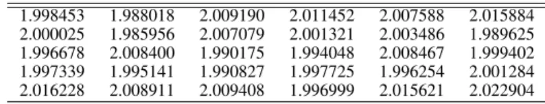
We will consider the data used in Nunes et al. [8]. In this research the authors generated samples with size 30 using R software, assuming the diameters and heights to be normal distributed with mean values 2 and 4, respectively, and standard deviation0.01. The results are presented in Tables1and2.The corresponding volumes are presented in Table3and the values ofY in Table 4.
Table 1. Values of diameters
1.998453 1.988018 2.009190 2.011452 2.007588 2.015884 2.000025 1.985956 2.007079 2.001321 2.003486 1.989625 1.996678 2.008400 1.990175 1.994048 2.008467 1.999402 1.997339 1.995141 1.990827 1.997725 1.996254 2.001284 2.016228 2.008911 2.009408 1.996999 2.015621 2.022904
Table 2. Values of heights
3.993445 4.002777 4.007956 3.992823 3.990726 3.998639 3.985255 3.997894 4.002110 4.009253 3.987402 3.989987 3.979206 4.015282 3.988615 4.010963 3.997377 3.994258 3.991256 3.993969 3.996335 3.996736 4.018685 3.996539 3.999213 3.987138 3.982822 3.982265 3.996033 3.998660
Table 3. Cylinders volumes
12.52638 12.42487 12.70734 12.68789 12.63255 12.76243 12.52036 12.38398 12.66216 12.61209 12.57050 12.40520 12.45956 12.72057 12.40780 12.52592 12.66469 12.54082 12.50555 12.48653 12.43995 12.52757 12.57782 12.57162 12.76861 12.63783 12.63040 12.47314 12.75078 12.85154 Table 4. Values ofY -0.003088 -0.010924 0.010883 0.009381 0.005109 0.015136 -0.003552 -0.014080 0.007395 0.003529 0.000319 -0.012443 -0.008247 0.011904 -0.012242 -0.003123 0.007590 -0.001972 -0.004695 -0.006164 -0.009759 -0.002996 0.000884 0.000406 0.015613 0.005517 0.004943 -0.007198 0.014237 0.022015
The p-value of the Kolmogorov-Smirnov test for normality, considering null mean value and varianceσ2= 0.012,
was 0.9052. So we don’t reject the hypothesis of normality ofY for the usual levels of significance. Taking the valuey = 0.022015ofY (randomly selected) we obtained
∥eµµµ∥ = 4.925884. In this case,S∼ χ2
58ands = 0.005.
The quantiles of eδ1/2, eδ1/2
q , are presented in Table 5.
Table 5. Quantiles of eδ1/2
Values ofq 0.9 0.95 0.99
e
δq1/2 645.8365 610.4035 591.7619
The high values obtained for these quantiles are due to the fact that we worked with small variance. So we can conclude that we are in a non-central situation in which the limit distributions, obtained through the asymptotic linearity, apply.
6. Final Remarks
With this research it was shown that the general results of the limit distributions apply when the error has spherical density, namely if it is normal. The numerical application on cylinder volume illustrates the usefulness of our approach. Moreover the approach presented for the normal case can be applied to Wishart matrices. Namely, we intend to publish results on limit distributions for these matrices, their trace and determinant. Others applications may be found in [2], [6] and [8].
Acknowledgement
This work was partially supported by national founds of FCT-Foundation for Science and Technology under UID/MAT/00212/2013 and UID/MAT/00297/2013.
REFERENCES
1. C. Fernandez, J. Osiewalski, M. Steel, Modelling&inference withν-spherical distributions. J. Amer. Statist. Assoc., vol. 90, no.
432, pp 1331 – 1340, 1995.
2. D. Ferreira, S.S Ferreira, C. Nunes, L. Ramos and J.T. Mexia, Approximate normality of low degree polynomials in normal
independent variables. Far East J. Math. Sci., vol. 68, no. 2, pp. 287 - 296, 2012.
3. D. Ferreira, S.S. Ferreira, C. Nunes and S. Incio, Inducing pivot variables and non-centrality parameters in elliptical distributions. 11th International Conference on Numerical Analysis and Applied Mathematics. AIP Conf. Proc., vol. 1558, pp. 833-836, 2013. 4. D. Ferreira, S.S. Ferreira, C. Nunes, M. Fonseca and J.T. Mexia, Chisquared and Related Inducing Pivot Variables: An Application
to Orthogonal Mixed Models. Communications in Statistics - Theory and Methods, 2013. doi:10.1080/03610926.2013.770532
5. M. Lo`eve, Probability Theory, 4th ed., New York, NY: Springer, 1977.
6. J.T. Mexia and M.M. Oliveira, Asymptotic linearity and limit distributions, approximations. J. Stat. Plan. Infer., vol. 140, no. 2, pp. 353-357, 2010.
7. J.T. Mexia, C. Nunes and M.M. Oliveira, Multivariate Application Domains for the Delta Method. In Proceedings of9th International Conference on Numerical Analysis and Applied Mathematics. AIP Conf. Proc. vol. 1389, pp. 1486-1489, 2011.
8. C. Nunes, M.M. Oliveira and J.T. Mexia, Application domains for the Delta method. Statistics, vol. 47, no. (2), pp. 317-328, 2013. 9. R.N. Rattihalli and P.Y. Patil, Generalizedυ-Spherical Densities. Communications in Statistics - Theory and Methods, vol. 39, no.
19, pp. 3568-3583, 2013.
10. M.M. Oliveira, Modelac¸˜ao de s´eries emparelhadas de estudos com estrutura comum. Unpublished PhD thesis, Universidade de ´Evora, 2002.