On the use of thermographic method to measure fatigue limits

(1)

Thematic Section: Solid Mechanics in Brazil 2017

On the use of thermographic method to measure fatigue limits

Abstract

Traditional fatigue limit measurements are expensive and time consuming, requiring a large number of specimens and a long time to be completed. An alternative approach is used in this work to obtain the fatigue limit of a cold drawn steel, in a rotating bending machine, by monitoring temperature variations induced by different load range levels in just a few specimens. Comparisons with Dixon’s traditional up-and-down method confirm that this thermographic approach is indeed a much more efficient, faster, and cheaper method to obtain fatigue limits.

Keywords

Fatigue, Fatigue limits, Thermographic method.

1 INTRODUCTION

The fatigue limit is a most important property for practical applications. It is widely used to avoid fatigue failures in long life structural designs, since it quantifies the stress amplitude below which macroscopic fatigue cracks should not initiate under alternated service loads. Since estimations of fatigue properties are intrinsically unreliable [1], experimental determination of fatigue limits is a must to warrant the reliability of engineering designs. Material fatigue limits S 'L can be measured by testing small polished specimens under constant amplitude alternated loads, while fatigue limits of structural components SL can be obtained by testing full size pieces [1]. Albeit traditional fatigue limit measurement techniques based on Dixon’s up-and-down sequential method may require fewer specimens than other approaches, they still need many specimens and very long testing times in universal servo-hydraulic or electromechanical testing machines, or even in dedicated rotating bending machines [2]. Even though, they still are the preferred method in practical applications to avoid coaxing, especially in ferrous alloys, which may induce fatigue strengthening under cyclic loading below but close to the fatigue limit. It may be a problem, for instance, when using Prot’s incremental method to measure fatigue limits [3-4].

Measurement techniques based on resonant ultrasonic tests, primarily used in very high cycle fatigue studies, can be used to speed up fatigue limit measurements by much increasing the test frequencies, but they are not widely applied in practice due to experimental difficulties [5-6]. Nevertheless, a recently proposed alternative thermographic method based on the measurement of temperature increments induced by various load amplitude levels can be a much more efficient, faster and cheaper way of assessing fatigue limits even without cracking the specimens. The main idea behind thermographic methods is that the transition from primarily elastic undamaging load events below the fatigue limit to cyclic elastoplastic damaging events above it is also associated with detectable temperature increments in the fatigue specimens.

De Finis et al. [7] investigated the fatigue behaviour of martensitic and precipitation hardening steels by means of the thermography technique. Their thermographic analyses take into account all heat sources involved in fatigue tests, with accurate measurement of temperature relative to dissipative phenomena and an automatable procedure proposition.

Carlos Filipe Cardoso Bandeiraa,b

Paulo Pedro Kenedib*

Jaime Tupiassú Pinho de Castroa

a_{Departamento de Engenharia Mecânica, Pontifícia}

Universidade Católica do Rio de Janeiro - PUC–Rio, Rio de Janeiro, RJ, Brasil. E-mail:

fillypebandeira@hotmail.com, jtcastro@puc-rj.br

b_{Programa de Pós-Graduação em Engenharia}

Mecânica e Tecnologia de Materiais, Centro Federal de Educação Tecnológica Celso Suckow da Fonseca - CEFET/RJ, Rio de Janeiro, RJ, Brasil. E-mail:

paulo.kenedi@cefet-rj.br *Corresponding author

http://dx.doi.org/10.1590/1679-78254331

Received: July 29, 2017

In Revised Form: February 06, 2018 Accepted: March 07, 2018

(2)

Fan et al. [8] showed that temperature evolution during the fatigue tests is closely correlated to internal microstructural changes. Good agreements were achieved between results predicted by thermographic techniques with traditional testing procedures.

Guo et al. [9] established an intrinsic energy dissipation model, based on the double exponential regression for one-dimensional distribution of specimen surface temperature variations. According to the authors, this energy method takes intrinsic dissipation as the fatigue damage indicator, eliminating the interference of internal friction on fatigue life evaluations. The analysis indicates that in high-cycle fatigue, processed under constant stress amplitude, the microstructure evolution is characterized by a stable intrinsic energy dissipation rate. They established that fatigue failure would occur after part of this intrinsic dissipation, due to microplastic deformation, has accumulated a threshold value, which would be a material constant independent of the loading history.

Huang et al. [10] proposed three new treatment methods to determine the fatigue limit, by relating the temperature response (caused by dissipated energy) with the applied stress amplitude, using a graphic method.

Palumbo and Galietti [11] proposed a new thermal method named thermoelastic phase analysis, which was used to evaluate the fatigue limit of martensitic steels. Their main idea was that the thermoelastic response of a material under fatigue loading is influenced by the presence of a heat source, which is related to a dissipative phenomenon associated to fatigue damage mechanism. Monitoring this thermoelastic parameter could provide the fatigue limit identification.

Wang et al. [12] explored the use of full-field temperature measurement by infrared thermography to identify the microplasticity evaluation in the very high cycle fatigue regime. An ultrasonic fatigue testing machine and an infrared image system were used to correlate the estimated plastic strain amplitude with the fatigue lives of the material through the Manson-Coffin law.

The main objective of this work is to compare the fatigue limit of a low carbon cold drawn steel measured by traditional techniques with the fatigue limit obtained by the thermographic methodology proposed by La Rosa and Risitano [13], to verify if this new technique can indeed be a viable option to obtain the material fatigue limit.

2 THEORY

Traditional and thermographic procedures to obtain fatigue limit measurements are briefly described next.

2.1 Dixon’s up-and-down method

The up-and-down method is an iterative statistical technique suitable to measure transition properties like the fatigue limit of materials. First, a specimen is tested under a stress amplitude level

 

_a ₁. If it breaks, the next specimen is tested under a stress amplitude

   

a ₂ a ₁ decreased by a constant value

σ



a, but if it doesn’t break after reaching a long and sufficiently high number of cycles N, the next specimen is loaded by a stress amplitude

   

a ₂ a ₁ increased by the same



σ

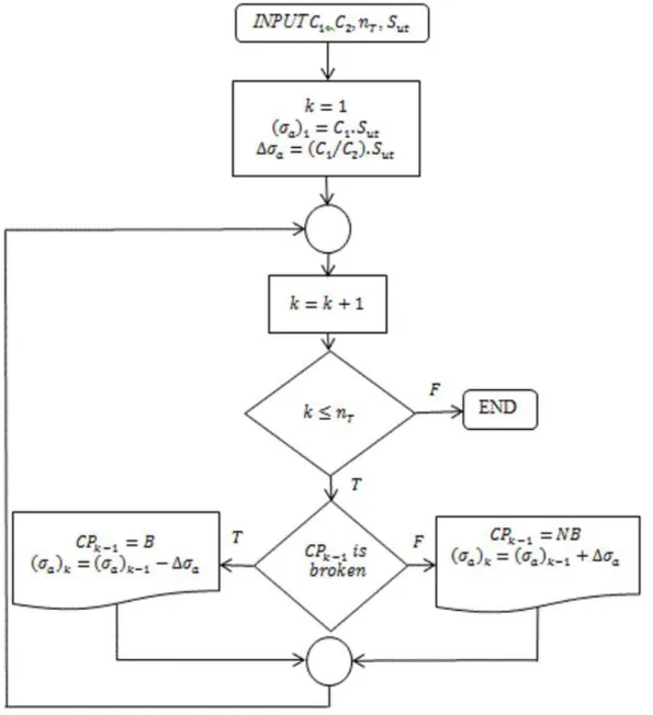
a [6]. This sequential process continues until a number of statistically representative number of specimens nT is tested [2].

Figure 1 shows a flowchart summarizing the up-and-down method, where 0 < C1< 1 is a constant that

multiplies the material tensile strength

S

ut to obtain the first stress amplitude level

 



a 1; C2 is another constant

(C2>1) used to generate the constant stress amplitude increment



σ

a; the integer counter

k

(1 k nT) is used to

define both the specimen’s number CPk and the stress amplitude level;

 



a _k; F and T represent a false and a

(3)

Carlos Filipe Cardoso Bandeira et al.

On the use of thermographic method to measure fatigue limits

Figure 1: Up-and-down method flowchart.

After testing all specimens, Dixon-Mood’s statistical analysis is used to estimate the fatigue limit following the flowchart presented in Figure 2, where:A,B,andCare constants calculated according to the equations defined in the flowchart.

When the less frequent event LFE is the survival, the number of stress amplitude levels tested on survived specimens is

q

max; then

m

q is the number of specimens that have survived at each stress amplitude level

q

. The

lowest stress amplitude level is always

 

a ₀, which is associated withq0.

However, if LFE is the failure, qmax represents the number of stress amplitude levels tested on failed

specimens; mq is the number of failed specimens at each stress amplitude level

q

. The lowest stress amplitude

level

 



a ₀ is also associated withq 0. The statistical analysis uses these parameters to determine the mean 

(4)

Figure 2: Dixon-Mood’s statistical analysis flowchart.

In this article, the up-and-down method is used as the reference method to measure the fatigue limit by means of standard rotating bending test procedures, as already done by other authors like Lipski [14], Curá et al. [15], La Rosa and Risitano [13] and Luong [16].

2.2 Thermographic method

It is well known that any material subjected to dynamic elastic loads slightly changes its temperature due to thermoelastic effects [17]. However, for loads above the fatigue limits these temperature variations are much more pronounced because fatigue damage necessarily involves dissipative cyclic plastic strains [13].

(5)

Figure 3: (a) Typical

T N



behaviour during cyclic loading; (b) Effect of the stress amplitude level.

Phases I, II and III in Fig. 3a represent the three thermal stages observed during a typical fatigue test. Phase I is characterized by a linear temperature increase from the test beginning until the change of its rate  T/ N_I to a lower value. It typically corresponds to about 10% of the number of cycles to failure for a specific load level [18]. Phase II is characterized by an increase rate  T/ NII smaller than the previous phase which could be zero for

some materials [16]. Finally, phase III is characterized by its abrupt temperature increase rate 𝜕𝑇/𝜕𝑁 >> 𝜕𝑇/ 𝜕𝑁 up to the final fracture.

Phase I can be associated to the fatigue starting process or to the crack nucleation stage, due to the formation of intrusions and extrusions primarily caused by the cyclic shear stresses parallel to the smallest crack surface. Phase II can be associated to the crack propagation stage, due to the dislocation movement inside plastic zones that is always ahead crack tips, which are primarily driven by the normal stresses perpendicular to crack surface. Phase III can be associated to fatigue instability condition, when the crack length approaches and reaches its critical length, causing sudden failure. Moreover, the curves T N, σ



a



reduces the temperature variation and increase the number of cycles to failure as the stress amplitude become closer to the fatigue limit '

L

(6)

adapted from [18]. On the other hand for

σ

a



S

L' the temperature does not change or changes very little, since

these low stress amplitudes do not start or propagate fatigue cracks [13, 18]. Note that apostrophe character used in fatigue limit symbol

S

L'

means that it is referred to the rotating-beam specimen.

Based on the typical T N behaviour of fatigue specimens, Risitano proposed to determine fatigue limits using phase I temperature variation TI or increase rate

 

T/ N

I for several stress amplitude levels, a task that

can be done using always the same specimen. To implement it, it was plotted

 

T σ

I a or   T/ N σI a, where

I 1 0

T T T

   is the temperature variation in the end of phase I, T1 is the maximum temperature in the end of phase

I and T0 is the specimen temperature when test begins. Risitano showed that  T σI a or   T/ N σI a have a

bilinear trend with very different slopes  

 

T / σI  a or   



T/ N / σI



 a, respectively. These two slopes can be

used to identify the transition from no fatigue damage below the fatigue limit to damage accumulation above it, and by consequence the fatigue limit of the tested specimen. According to Risitano, operationally the fatigue limit

' L

S can be determined by thermographic technique extending the straight line with highest slope until it across

σ

a

-axis. This approach will be used in this article.

3 MATERIAL AND METHODOLOGY

Basic material properties were obtained through chemical analysis, tensile tests and metallography. Fatigue tests were made in a rotating bending machine under load ratio R 1 and frequency f 8,500 Hz, enough to reach the proposed number of cycles to characterize an infinity life _N _{5 10}6

  cycles in about 10 hours, supposing as usual that the fatigue limit of steels is determined for lives less than _{1 10}_ 6_{cycles. In the thermography tests}

the specimen surface temperature was measured by an infrared camera. Temperature increase rate of first thermal phase was determined at several stress amplitude levels in order to plot   T/ N σI a and determine the

fatigue limit.

3.1 Material characterization

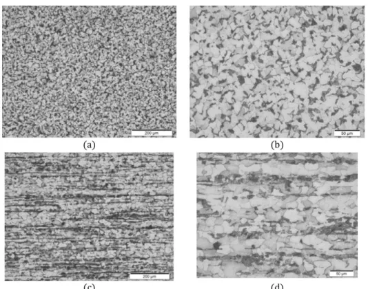
Table 1 lists the chemical composition of the low carbon steel used in this article. The mean value of its tensile properties obtained in 3 tests is presented in the Table 2, where S_y is the yield strength, Sut is the tensile strength and RA is the area reduction percentage.

Table 1: Chemical composition (%).

C Si Mn P S Cr Ni Mo Al Cu Ti Nb V

0.226 0.114 0.510 0.020 0.0028 0.024 0.011 0.003 0.017 0.026 <0.001 <0.003 0.001

Table 2: Tensile properties.

y

S

(MPa)

S

ut (MPa) (%) RA

576.6 666.6 50.1

(7)

Figure 4: Micrographies: transversal: (a) 200X; (b) 500X; longitudinal: (c) 200X; (d) 500X.

3.2 Specimen geometry

The specimens followed ASTM E466 standard [20], see Fig. 5a and 5b. All specimens were machined from the same raw material batch in a CNC lathe, using small cutting feeds. The mean surface roughness was measured

0.78



a

R µm, equivalent to a N6 ground finishing [21]. Figure 5c shows a specimen with its central part black painted to increase its emissivity in order to improve infrared camera performance in the thermographic tests. All specimens were dimensionally checked and stored in a humidity controlled environment.

(8)

3.3 Test equipment

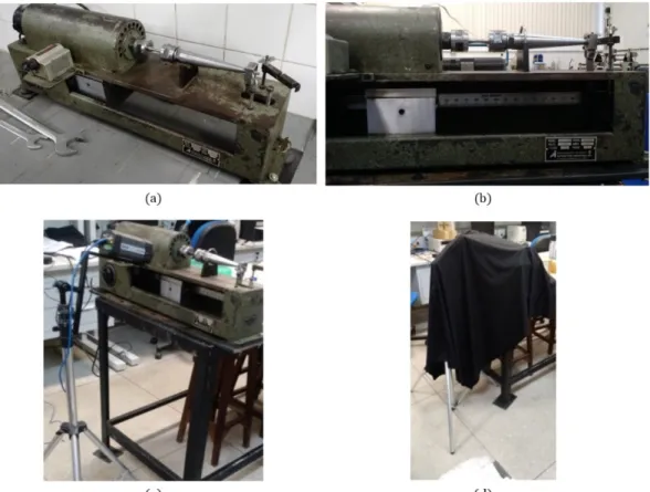
A rotating bending machine RBF 200 was used in all fatigue tests. It works by bending moment application on specimen by positioning a block with a constant mass on a ruler. Each position indicates the applied bending moment in the central cross section of specimen, the supposed critical region, in such a way that to increase or to decrease the specimen stress amplitude level it is only a matter of repositioning the mass. The great advantage of this machine is the load frequency, which can achieve up to 10,000 rpm. Figure 6 shows the RBF 200 used in this article.

Figure 6: RBF 200: (a) overview; (b) lateral view; Thermographic system: (c) infrared camera and (d) black cloth.

In the thermographic test, the specimen surface temperature was continuously measured by an infrared camera FLIR A320, with resolution 320 x 240 pixels, data acquisition frequency 30Hz and temperature sensibility 50mK. The temperature data was analyzed using the software ResearchIR from FLIR. The surface of all specimens was black painted to increase its emissivity, as shown by Fig. 5.c. In additon, a black cloth was used to cover the rotating bending machine and camera. Figure 6.c shows the thermographic system with the infrared camera and Fig. 6.d shows the black cloth.

3.4 Test method

For up-and-down method, the stress amplitude increment was set as  a 0.02 S ut. The number of cycles to

characterize an infinite life was set as _N _{5 10}6

  cycles. The first specimen was tested under

 



a ₁0.4Sut and

25

t

n  specimens were tested in total.

For thermographic method, initially the surface temperature of one specimen was continuously monitored until its failure under óa = 0.6·Sut, in order to study the material three thermal phases behaviour. To find the

fatigue limit, four specimens were tested under increasing stress amplitude steps

 

σa k/Sut = 0.35, 0.40, 0.44,

0.48, 0.50, 0.52, 0.54, and 0.6, each one lasting the number of cycles necessary to characterize the first thermal

phase 3

I

N 5 10  cycles, measured in the previous tests. After finding the various phase I temperature rates for each specimen, their 𝜕T/𝜕N1×óa/Sut curves were plotted to access the fatigue limit measured by thermographic technique '

(9)

4 RESULTS

The results obtained with up-and-down and thermographic methods are presented next.

4.1 Up-and-down method

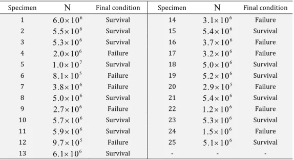
Figure 7 shows the results obtained for each tested specimen and Table 3 shows the number of cycles

N

that each specimen resisted with its associated final condition: failure or survival.

Figure 7: Up-and-down fatigue test results.

Table 3: Final condition for each tested specimen.

Specimen

N

Final condition Specimen

N

Final condition

1 6.0 10 6 Survival 14 3.1 10 6 Failure 2 5.5 10 6 Survival 15 5.4 10 6 Survival 3 _{5.3 10}_ 6 _Survival ₁₆ _{3.7 10}_ 6 _Failure 4 _{2.0 10}_ 6 _Failure ₁₇ _{3.2 10}_ 6 _Failure 5 _{1.0 10}_ 7 _Survival ₁₈ _{5.0 10}_ 6 _Survival 6 8.1 10 5 Failure 19 5.2 10 6 Survival 7 3.8 10 6 Failure 20 2.9 10 5 Failure 8 _{5.0 10}_ 6 _Survival ₂₁ _{5.4 10}_ 6 _Survival 9 _{2.7 10}_ 6 _Failure ₂₂ _{1.2 10}_ 6 _Failure 10 _{5.7 10}_ 6 _Survival ₂₃ _{5.3 10}_ 6 _Survival 11 5.9 10 6 Survival 24 1.5 10 6 Failure 12 9.7 10 5 Failure 25 5.1 10 6 Survival

(10)

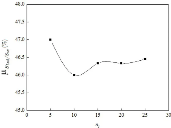
Note that the mean fatigue limit measured by the traditional up-and-down has a convergence tendency because it depends on the total number of tested specimens nT. Figure 8 shows that mean fatigue limit tended to

converge starting at 15 tested specimens. In this article it was used the mean value calculated for n 25T .

Figure 8: Mean fatigue limit convergence obtained by up-and-down procedure.

The up-and-down approach results were then used with Dixon-Mood’s statistical method to calculate the mean value and standard deviation of the fatigue limit, considering the less frequent event as the failure, as summarized in the Table 4.

Table 4: Fatigue limit obtained from traditional up-and-down method.

μ

(%)

φ

(%)

' _

L ud

S

(MPa)

46.3 1.1 308.9 ± 7.1

4.2 Thermographic method

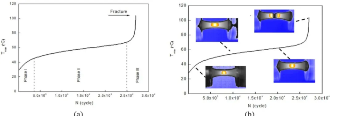
Figure 9a depicts the tesulting TmaxN curve for σ 0.6 Sa  ut. It shows that the phase I is characterized by a small number of cycles ( 3

I

N 5 10  ); the phase II includes most of the specimen life ( 4 II

N  2 10 ); the phase III is associated with a sudden temperature increase, where the specimen final fracture occurs in a small number of cycles (NIIINI). Figure 9b shows some pictures of the temperature distribution on the specimen surface for the three thermal phases and final rupture. They show that, as expected, the higher temperatures are localized around the smaller section of the specimen, where the final fracture occurred.

(11)

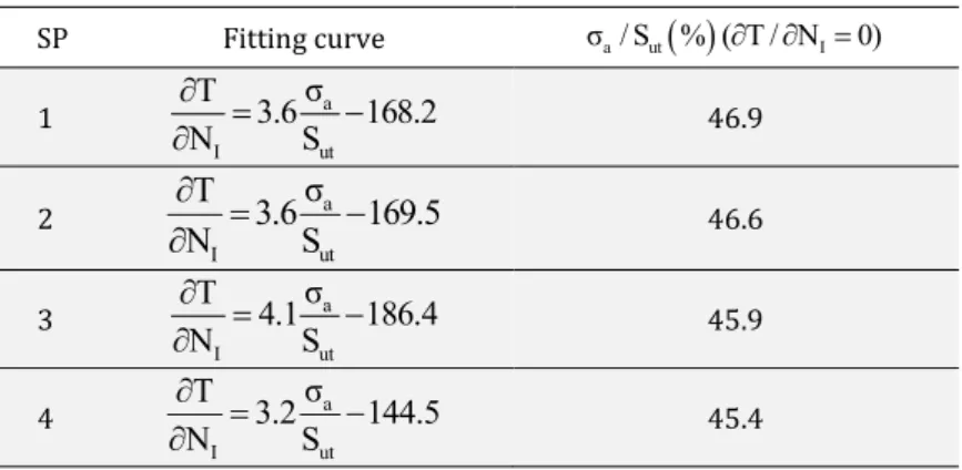
amplitude of each load step. Figure 12 show the relation between stress amplitude value and temperature increase rate of phase I. Figure 12 also presents the linear fitting using the least square method, done with the experimental points with 𝜕T/𝜕N1>0.1 T / N σ /S  I



a ut0.35



. The fitting curve equations and their associated

fatigue limit estimative (  T/ N 0I ) are described in Table 5.

Figure 9: Temperature distribution for

σ

a

 

0.6 S

ut: (a)

T

max



N

curve; (b) temperature evolution.

(12)

Figure 11: TmaxN under increasing load steps.

(13)

Table 5: Fitting curve equations.

SP Fitting curve σ / S % ( T / N 0)a ut

 

  I

1 a

I ut

σ

T 3.6 168.2

N S

 _ _

 46.9

2 a

I ut

σ

T 3.6 169.5

N S



 

 46.6

3 a

I ut

σ

T 4.1 186.4

N S

 _ _

 45.9

4 a

I ut

σ

T 3.2 144.5

N S

 _ _

 45.4

Using the results from Table 5, it is possible to determine the mean value and the standard deviation of the fatigue limit, as presented in Table 6.

Table 6: Fatigue limit by the thermographic approach.

μ

(%)

φ

(%)

 

'

_ /S ) %ut L th

S S'L th_

(MPa)

46.2 0.7 46.2 ± 0.7 307.2 ± 4.7

5 DISCUSION

The fatigue limit '

_ /S UT L ud

S = (46.3 ± 1.1)%, measured by traditional up-and-down procedures needed 25 specimens to achieve a stable value, with a relatively small dispersion. The fatigue limit determined by the thermographic method '

_ /SUT L th

S = (46.2 ± 0.7)% was surprisingly close to and slightly less disperse than the one obtained by the reference procedure, with the results obtained in a much faster way.

Indeed, the thermographic tests used 8 specimens, but could have used only 5 specimens (1 for establish the thermal phases and 4 to obtain the fatigue limit), a task that can be easily completed in only one day of work without even breaking them. Moreover, they yielded essentially the same fatigue limit measured by sequentially testing by up-and-down standard procedures 25 specimens up to failure, or else to run-out after at least _{5 10}_ 6

cycles (a much more laborious task that required about one month of work.)

It is interesting to note that such values are compatible with classic estimates for low-carbon steel components with ground surfaces, namely '

UT 0.45 S L

S   as defined in reference [1], a reassuring fact for structural designers.

Finally, although outside the scope of this work, it is necessary to mention that the fatigue limit is just part of the problem when designing for very long, or for hopefully “infinite” lives. While microstructural defects such as inclusions and voids are intrinsically included in SL, small scratches, corrosion pits, and similar incidental surface

defects, practically unavoidable in long service lives, may affect the crack initiation process. So, although not yet recognized by most designers or by codes, to avoid crack initiation in any structural component it must be able to resist the service loads in the presence of the most damaging (small) defect it may acquire during its operational life.

In other words, structural components that must last for very long fatigue lives should be designed to work under stresses below their fatigue limits and to be tolerant to undetectable short cracks. Indeed, continuous work under fatigue loads cannot be guaranteed if any of the flaws that they might have can somehow propagate during their service lives. However, despite self-evident, this prudent requirement is still not included in SN or åN fatigue design routines used in practice. Indeed, most long-life designs just intend to maintain the service stresses at the structural component’s critical point below its fatigue limit, Äó < ÄSLR/ϕF, where ϕF is a suitable safety factor for

fatigue applications. So, although such calculations can be quite complex (e.g. when analyzing fatigue crack initiation caused by random multiaxial non-proportional loads), their so-called safe-life philosophy is not that safe.

(14)

much tolerant” cannot be answered by SN or åN procedures alone. This potentially important problem can be dealt with by adding short crack concepts to their infinite life design criteria using Fracture Mechanics tools, see for instance [22-23] for further details.

6 CONCLUSION

Thermographic techniques originally proposed by Risitano proved to be really a much faster and easier way to obtain the fatigue limit of the tested low carbon steel. The utilization of a rotating bending machine to access the fatigue limit for both techniques, up-and-down and thermographic, with R = −1, produced similar results, yielding values directly comparable with the majority of the available fatigue limits. This new technique proved to have many advantages in relation to classical techniques to obtain fatigue limits, such as the utilization of fewer specimens and the access to the fatigue limit without the necessity of leading the specimens to final failure (complete rupture). Therefore, in the authors opinion, it is time to seriously consider a round-robin to evaluate the possibility of standardizing these thermographic procedures for use in practical applications.

7 REFERENCES

[1] Castro, JTP; Meggiolaro, MA., 2016, Fatigue Design Techniques, vol. 1: High-Cycle Fatigue.

[2] Pollak, R.; Palazotto, A.; Nicholas, T., 2006, “A simulation-based investigation of the staircase method for fatigue strength testing”, Mechanics of Material, 38, 1170-1181.

[3] Corten,HT; Dolan,TJ. 1953, An appraisal of the Prot method of fatigue testing, part II. Technical Report 35, ONR.

[4] Kerscher,E; Lang,KH; Vohringer,O; Lohe, D. 2008, ”Increasing the fatigue limit of a bearing steel by dynamic strain ageing”. International Journal of Fatigue 30:1838-1842.

[5] Bathias, C.; Paris, P. C., 2005, “Gigacycle fatigue in mechanical practice”, Marcel Dekker, New York.

[6] Nicholas, T., 2006, “High cycle fatigue – A mechanics of materials perspective”, chapter 3, Elsevier, Great Britain.

[7] De Finis, R.; Palumbo, D.; Ancona, F.; Galieti, U., 2015, “Fatigue limit evaluation of various martensitic stainless steels with new robust thermographic data analysis”, International Journal of Fatigue 74:88–96.

[8] Fan, J.; Guo, X.; Wu, C.; Crupi, V.; Guglielmino, E., 2013, “Influence of Heat Treatments on Mechanical Behavior of FV520B Steel”, Experimental Technics, 39:55-64.

[9] Guo, Q.; Guo, X.; Fan, J.; Syed, R; Wu, C., 2015, “An energy method for rapid evaluation of high-cycle fatigue parameters based on intrinsic dissipation”, International Journal of Fatigue, 80:136-144.

[10] Huang, J.; Pastor, M.; Garnier, C.; Gong, X., 2017, “Rapid evaluation of fatigue limit on thermographic data analysis”, International Journal of Fatigue, 104:293–301.

[11] Palumbo, B.; Galietti, U.; 2017, “Thermoelastic Phase Analysis (TPA): a new method for fatigue behaviour analysis of steels”, Fatigue & Fracture of Engineering Materials & Structures, 40:523-534.

[12] Wang, X. G.; Feng, E. S.; Jiang, C., 2017, “A microplasticity evaluation method in very high cycle fatigue”, International Journal of Fatigue, 94:6–15.

(15)

[14] Lipski, A., 2016, “Accelerated determination of the fatigue limit and the S-N curve by means of the thermographic method for X5CrNi18-10 steel”, Acta Mechanica et Automatica, vol. 10, 22-27.

[15] Curà, F.; Curti, G.; Sesana, R., 2005, “A new iteration method for the thermographic determination of fatigue limit of steels”, International Journal of Fatigue, vol. 27, 453-459.

[16] Luong, M. P., 1998, “Fatigue limit evaluation of metals using an infrared thermographic technique”, Mechanics of Materials, vol. 28, 155-163.

[17] Pitarresi, G.; Patterson, E.A., 2003. A review of the general theory of thermoelastic stress analysis. J Strain Analysis 38:405-417.

[18] Fargione, G.; Geraci, A.; La Rosa, G.; Risitano, A., 2002, “Rapid determination of the fatigue curve by the thermographic method”, International Journal of Fatigue, vol. 24, 11-19.

[19] Risitano, A.; Risitano, G., 2010, “Cumulative damage evaluation of steel using infrared thermography”, Theoretical and Applied Fracture Mechanics, vol. 54, 82-90.

[20] ASTM E466, 2015, “Standard practice for conducting force controlled constant amplitude axial fatigue tests of metallic materials”, chapter 5.

[21] Smith, Graham T., 2002, “Industrial Metrology – Surfaces and Roundness”, Springer.

[22] Castro, J.T.P.; Meggiolaro, M.A.; Miranda, A.C.O.; Wu, H.; Imad, A.; Nouredine, B., 2012, Prediction of fatigue crack initiation lives at elongated notch roots using short crack concepts. Int J Fatigue 42:172-182.