doi: 10.5540/tema.2018.019.01.0111
Arboreal Identification Supported by Fuzzy Modeling for
Trunk Texture Recognition
A. BRESSANE1*, F.H. FENGLER2, S.R.M.M. ROVEDA2, J.A.F. ROVEDA2and A.C.G. MARTINS2
Received on March 19, 2017 / Accepted on January 22, 2018
ABSTRACT. Due to the natural variability of the arboreal bark there are texture patterns in trunk images with values belonging to more than one species. Thus, the present study analyzed the usage of fuzzy mod-eling as an alternative to handle the uncertainty in the trunk texture recognition, in comparison with other machine learning algorithms. A total of 2160 samples, belonging to 20 tree species from the Brazilian native deciduous forest, were used in the experimental analyzes. After transforming the images from RGB to HSV, 70 texture patterns have been extracted based on first and second order statistics. Secondly, an exploratory factor analysis was performed for dealing with redundant information and optimizing the computational effort. Then, only the first dimensions with higher cumulative variability were selected as input variables in the predictive modeling. As a result, fuzzy modeling reached a generalization ability that outperformed some algorithms widely used in classification tasks. Therefore, the fuzzy modeling can be considered as a competitive approach, with reliable performance in arboreal trunk texture recognition.
Keywords: soft computing, image processing, pattern matching, bioinformatics.
1 INTRODUCTION
The usage of computational intelligence in the feature extraction and pattern recognition from biological data has been increasingly studied for supporting the arboreal identification. However, as the studies carried out have focused on the processing of leaf images, these techniques are not applicable when the leaf structure is not available, as occurs with deciduous species at certain times of the year.
As an alternative, the texture recognition in tree trunk images still has few outcomes reported in the literature, in which the predictive modeling has been performed using machine learning
*Corresponding author: Adriano Bressane – E-mail: [email protected].
1Faculdade de Engenharia de Sorocaba (Facens), Campus at Sorocaba city, S˜ao Paulo State, Rodovia Senador Jos´e Erm´ırio de Moraes, 1425, Brazil.
2Universidade Estadual Paulista (Unesp), Campus at Sorocaba city, 03 March Avenue, 511, Brazil.
algorithms based on k-Nearest Neighbors ([26], [30]), Artificial Neural Networks ([19]), Support Vector Machine ([6], [13], [18]), and Decision Tree ([10]).
By analyzing statistical properties in tree trunk images, [10] found that, due to the natural vari-ability of the arboreal bark, commonly its texture patterns have some values belonging to more than one species, i.e, there is an overlap between neighboring subspaces. As a consequence, this overlapping in the pattern matching can lead to an ambiguity during predictive modeling.
In these cases, there is some uncertainty with regard to what species the sample belongs to, un-dermining the texture analysis by means of predictor variables with a sharply defined boundary. Therefore, the present study aims to analyze the usage of fuzzy modeling as an approach to deal with the uncertainty in the trunk texture recognition, in comparison with other machine learning algorithms.
In the mid-1960s, the fuzzy set theory has been developed by [32] as an extension of the classical set theory to provide a mathematical treatment for complex phenomena, becoming it popular after 1980s ([33], [25]). For that, the fuzzy modeling is a soft-computing method capable of processing uncertain knowledge or data. Thus, by affording a convenient formalism for integrating different kinds of variables, by means of an user-friendly structure with transparency and interpretability, the usage of fuzzy modeling is becoming more and more common, with several applications in the environmental sciences over the years (e.g. [7], [8], [9], [22], [23], [21], [4], [2], [28]).
According to [20], the main applications of the fuzzy modeling used to be optimization and control problems. Nevertheless, nowadays many other areas can be highlighted, such as the de-velopment of intelligent systems for supporting the decision making, data mining, signal pro-cessing, diagnosis, forecasting, regression, and classification from numerical data using pattern recognition based on the graded membership ([29]). Thereby, the fuzzy modeling can achieve a competitive performance when compared to other machine learning algorithms in classifica-tion tasks involving uncertainty, vagueness, partial true, which demand predictors without hard boundaries ([3], [27]).
2 METHODS
2.1 Data collection and feature extraction
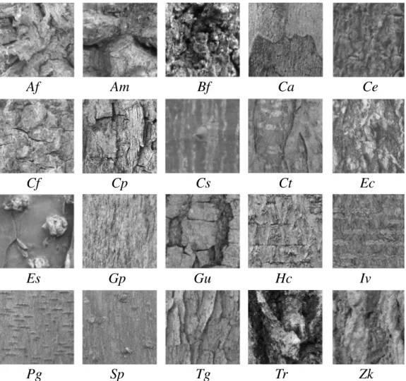
The data were collected using a digital camera for capturing outer bark images at different heights of the trunk, at a 50 mm distance around the trees. Due to the three-dimensional shape of arboreal trunk, only a central area was used for extracting features, in order to avoid the distortion at the image edge. Then, using a moving mask with 512 x 512 pixels, 2160 samples were obtained, being 108 of each of the 20 tree species from the Brazilian native deciduous forest, shown in Figure 1.
Af
Am
Bf
Ca
Ce
Cf
Cp
Cs
Ct
Ec
Es
Gp
Gu
Hc
Iv
Pg
Sp
Tg
Tr
Zk
Figure 1: Tree trunk images (512x512 pixels) from: Anadenanthera falcata (Af), Anadenan-thera macrocarpa(Am),Bauhinia forficate(Bf),Caesalpinia ferrea(Ca),Caesalpinia echinata (Ce),Cedrela fissilis(Cf),Caesalpinia peltophoroides(Cp),Ceiba speciosa(Cs),Centrolobium tomentosum(Ct),Enterolobium contortisiliquum(Ec),Erythrina speciosa(Es),Gochnatia poly-morpha (Gp),Guazuma ulmifolia(Gu),Hymenaea courbaril(Hc),Inga vera(Iv),Piptadenia gonoacantha(Pg),Schizolobiun parahyba(Sp),Tibouchina granulosa(Tg),Tabebuia roseoalba (Tr), andZanthoxylum kleinii(Zk).
tem to HSV (hue-saturation-value) space. Then, features based on first and second order statistics were extracted using the V channel from the grayscale images.
As a measure of the proximity of the gray levels, the uniformity (u) is given by:
u=
L−1
∑
i=0
p2(zi) (2.1)
whereLcorrespond to the number of gray levels in the image,ziis the intensity, andp(zi)is the
image histogram.
The first-order entropy (e) measures the randomness in the image, as in:
e=−
L−1
∑
i=0
p(zi)log2p(zi) (2.2)
The skewness is a measure of the asymmetry (µ3), and smoothness (s) takes in to account the
transition of gray shades, respectively obtained by:
µ3=
L−1
∑
i=0
(zi−µ1)2p(zi) (2.3)
and
s=1− 1
1+µ2 2
(2.4)
where (µ1) is the intensity that returns the gray level average, and (µ2) is the standard deviation,
calculated by:
µ1=
L−1
∑
i=0
zip(zi) (2.5)
and
µ2=
1 n−1
n
∑
i=1
(zi−µ1)2 (2.6)
wherenis the number of image pixels.
In turn, the second order statistics was composed of the contrast, correlation, energy, and homo-geneity, measured at 16 positions (φ), correspondent to distance between pixels equal to 1, 3, 5 and 7, in the rotation angles 0, 45, 90 and 135 degrees, producing 64 texture features. These descriptors are described below from [17] and [15].
Contrast (c) compares the intensity of neighboring pixels, being calculated by:
cφ=
k
∑
i=1
k
∑
j=1
(i−j)2p
i j (2.7)
wherekis the co-occurrence matrix dimension,pi jis probability of satisfyingφ.
The correlation (r) measures the probability of occurrence of specified pixel pairs, given by:
rφ =
k
∑
i=1
k
∑
j=1
(i−mrow)(j−mcol) σrow−σcol
Energy (ε) adds the squared elements in the co-occurrence matrix, and homogeneity (h) measures the closeness of gray levels in the spatial distribution over image, respectively obtained by:
εφ=
k
∑
i=1
k
∑
j=1
p2i j (2.9)
and
hφ=
k
∑
i=1
k
∑
j=1 pi j
1+|i−j| (2.10)
From the foregoing, the total number of measured variables amounted to 70 texture features. Then, taking into account that some features may be highly correlated, an Exploratory Factor Analysis (EFA) has been performed. As a multivariate analysis technique, the EFA finds a coor-dinate system that maximizes the variance shared among variables, enabling to reduce the data dimensionality and prevent the use of redundant information ([12]).
In the new m-dimensional space found by EFA, the standardized original variables (z) correspond to linear combinations of underlying factors (z′), given by ([31]):
zj=aj1z′1+aj2z′2+...+ajmz′m (2.11)
For that, the EFA was carried out using the Spearman’s coefficient, a non-parametric alternative regarded as robust for general distributions (non-normal data), the principal factors as extraction method, and the communalities (hi) based on the squared multiple correlations, as in:
hi= m
∑
j=1
li j2 (2.12)
whereli j is the correlation between the ith principal factor with jth original variable (texture
feature), previously standardized by means of:
zi=
xi−x¯
σ (2.13)
where xi is the measured original variable, ¯x and σ are respectively its mean and standard
deviation.
Thus, the features extracted from tree trunk images have been reduced to fewer latent variables (principal factors), which were used as predictors for generating fuzzy if-then rules in the texture pattern recognition.
2.2 Fuzzy modeling for the pattern recognition
For the predictive modeling in the present study, we used a fuzzy rule-based classification sys-tem, created and described by [27] as FRBCS.W algorithm, made available in R programming language by means of the ‘frbs’ package. The FRBCS.W algorithm has been developed based on the Ishibuchi’s method ([20]).
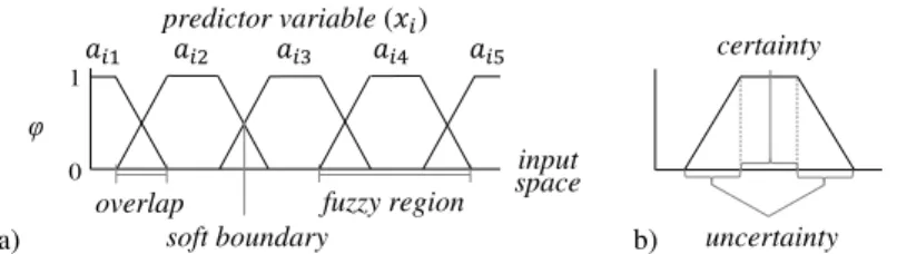
As aforementioned, the Ishibuchi’s method is a learning method from numerical data that consists of the fuzzy partitioning with certainty grades. In the learning process, the antecedent part of rules is determined by a grid-type fuzzy partition. This partitioning occurs by dividing the input space of the predictor variables (xi) into regular fuzzy regions, resulting in uniform and symmetrical
intervals correspondent to the antecedent terms (ai j), as can be seen in Figure 2.
φ
1
0
fuzzy region overlap
soft boundary
φ
soft boundary uncertainty
certainty
1
predictor variable ( )
input fuzzy region
overlapoverlap
a) b)
φ
uncertainty
b)
space
Figure 2: Grid-type fuzzy partition: (a) partitioning of the pre-dictor variable -xi; (b) intervals of certainty and uncertainty that
comprises the fuzzy region.
By using the grid-type fuzzy partition, the total number of rules (N) is determinate by amount of possible combinations of the antecedent terms. For that, rulebase is generated by pattern match-ing, calculating membership degrees (ϕ) of the training data in the antecedents terms (ai j) of
each predictor variable (xi). In turn, the consequent part is defined as the dominant categorical
variable (Cj) in the decision area formed by the fuzzy if-then rule ([20]):
RuleRj: IF x1isa1jAND...ANDxmisam j
THEN CjwithCFj, j=1,2, ...,N (2.14)
wherexis a m-dimensional vector of predictor variables (xi),CFj is the certainty grade of the
ruleRj, andCjis the dominant categorical variable, determined taking into account:
∑
p∈classCj
ϕj(xp) =max
(
∑
p∈class k
ϕj(xp):k=1,2, ...,c
)
(2.15)
wherexp= (xp1, ...,xpm)is a new pattern, and c is the number of output classes.
After generating the predictive model, the classification of new instances is based on a single winner rule, which is determined by ([20]):
ϕj(xp).CFj=max
whereϕj (xp) is the compatibility grade of the instance in the ruleRj, andCFj is the certainty
grade, a real number in the interval [0, 1] that works as the weight of rule, given by:
CFj=
βclassCj(Rj)−β¯
c
∑
k=1
βclass k(Rj)
(2.17)
where
¯
β=
∑
k6=Cj
βclass k(Rj)
(c−1) (2.18)
and
βclass k(Rj) =
∑
xp∈class kϕj(xp),k=1,2, ...,c (2.19)
2.3 Benchmarking experiment
From the database with 2160 samples, we used 70% of this total, randomly selected, for the ma-chine learning process. During this process a 5-fold cross-validation was carried out over learning dataset, in order to find the best control parameters setting. Then, a hold-out validation has been performed using the remaining 30% as testing dataset for assessing the generalization ability of the Fuzzy Rule-Based Classification System (FRBCS) in the trunk texture pattern recognition (Figure 3).
database
learning
testing training
checking
model
hold-out validation cross-validation
Figure 3: Split of database for the learning process and to assess the generalization ability based on testing dataset.
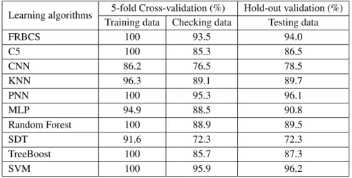
Furthermore, as a reference for assessing the performance from the fuzzy-based approach, a benchmarking experiment has been carried out using the same database for training, checking and testing other algorithms shown in Table 1.
Based on the testing results, the learning algorithms performance has been assessed according to the overall accuracy (θ), which measures the ratio of samples correctly classified by the total number of samples (nT), as in:
θ=n−T1
nsp
∑
i=1
T Pspi (2.20)
whereT Pspi is the total number of true positive samples, and nsp is the total number of tree
Table 1: Algorithms and setting of control parameters adjusted during the learning process, which provide the best results in the cross-validation over the checking dataset.
Learning algorithm Control parameters settings Available in Fuzzy-Based System frbcs.w, mf: gaussian, Package ‘frbs’
(FRBCS) t-norm: product, R language
antecedent terms: 23
Boosted Rule-Based subset: false, no global Package ‘C5.0’ Model (C5) pruning: false, CF: 0.25, R language
trials: 100
Cascade-Correlation kernel: sigmoid and Algorithm ‘CNN’ Neural Network (CNN) gaussian, neuron: 0-103, C language
candid. 102, epoch 103 prune to optimal size
k-Nearest Neighbors model: knn kernel, Pack ‘CORElearn’
(KNN) weighting: gaussian R language
kernel, type: probability
Probabilistic Neural sigma: each var., steps 20, Algorithm PNN Network (PNN) kernel: gaussian, prior prob.: C language
frequency distribution
Multilayer Perceptron layers: 3, overfitting control: Algorithm MLP Network (MLP) min. holdout val. error over C language
10% train, function: logistic
Random Dec. Forest importance: true, Pack ‘randomForest’ (Random Forest) proximity: true, R language
number of trees: 300
Single Decision Tree minimum node to split: 3, Algorithm SDT (SDT) maximum tree levels: 300, C language
prune to min cross-val error
Stochastic Gradient trees: 300, depth: 8, Algor. ‘TreeBoost’ Boosting (TreeBoost) min size node to split: 10, C language
prune series to min. err, minimum trees in series: 10
Support Vector type: bound-constraint, Package ‘kernlab’ Machine (SVM) kernel function: gaussian, R language
3 RESULTS AND DISCUSSION
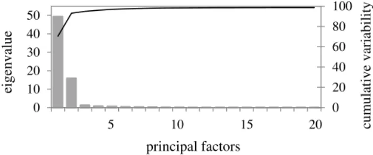
Regarding the requirements for data preprocessing using multivariate analysis, the Cronbach’s alpha equivalent to 0.9 indicated an excellent internal consistency, and the Kaiser-Meyer-Olkin equal to 0.97 confirmed a good sampling adequacy, verifying sufficient conditions to perform the Exploratory Factor Analysis (EFA), whose result is shown in Figure 4.
0 20 40 60 80 100
0 10 20 30 40 50
1 5 9 13 17 cum
ulat
ive
var
iabi
li
ty
eige
nvalue
principal factors
5 10 15 20
Figure 4: Eigenvalues and cumulative variability explained by the first 20 latent variables (principal factors) produced from the Exploratory Factor Analysis.
From the Figure 4, we find that the first 20 principal factors explain 99.0% of the cumulative variability. Therefore, the EFA was capable of reducing the data dimensionality and at the same time retaining almost all information available in the 70 original variables. Thus, these principal factors were used as predictor variables in the modeling process, affording the results shown in Table 2.
In general, each machine learning algorithm has properties which can provide better performance than others, depending on the characteristics of the case under analysis. Thus, the performance from the algorithms in the benchmarking experiment has been discussed taking into account such properties. In this sense, by analyzing Table 2 it is noted three performance groups according to the accuracy over testing dataset.
With accuracy less than 80%, in the first group are the Single Decision Tree (SDT) and Cascade-Correlation Neural Network (CNN). The CNN is a self-organizing network that determines its own size and topology, by adding neurons to the architecture. The SDT also grows adding nodes to its structure, both for reaching greater preciseness during the learning process. As a conse-quence, these algorithms can lead to an overfitting to the train data, losing some generalization ability. Then, we use an overfitting control pruning the models to minimum cross-validated error over checking dataset.
Table 2: Performance of the machine learning algorithms in the benchmarking experiment, using the first 20 principal factors as predictor variables.
Learning algorithms 5-fold Cross-validation (%) Hold-out validation (%) Training data Checking data Testing data
FRBCS 100 93.5 94.0
C5 100 85.3 86.5
CNN 86.2 76.5 78.5
KNN 96.3 89.1 89.7
PNN 100 95.3 96.1
MLP 94.9 88.5 90.8
Random Forest 100 88.9 89.5
SDT 91.6 72.3 72.3
TreeBoost 100 85.7 87.3
SVM 100 95.9 96.2
Capable of handling this issue better than the single tree-based model (SDT), the Decision Tree Forest (Random Forest), Stochastic Gradient Boosting (TreeBoost), and Boosted Rule-Based Model (C5.0) are in the second group of algorithms with medium-performance in the testing (from 80 to 90%), along withk-Nearest Neighbors (KNN).
The Random Forest and TreeBoost are ensembles based on different strategies of creating a collection of decision trees. The Random Forest uses the bagging (Bootstrap Aggregating) tech-nique for creating trees grown in parallel, which afforded a generalization ability of 89.5%. On the other hand, the TreeBoost uses a sequential training (boosting) that resulted in a series of trees with 87.3% accuracy. Similarly, C5.0 is a voting classification algorithm also based on a boosting technique to create a collection of rules that achieved 85.3% accuracy. The boosting usually provides more accuracy than bagging strategy, except when there is some noise in data, such as outliers ([5]). Therefore, as the Random Forest outperforms the boosting-based models in the present analysis, we can consider some influence of outliers. Notwithstanding, as the bark texture in the arboreal trunk is a biological feature subject to imperfections, these outliers has not been removed because they can be caused by a natural variability. In turn, the KNN is a non-parametric algorithm of instance-based learning, in which a pattern is recognized by ma-jority voting according to the similarity with theknearest neighbors. By using kernel functions to weight the vote of the neighbors, the KNN provides 89.7% accuracy, slightly higher than ensemble-based models.
The SVM operates by finding an n-dimensional hyperplane in order to optimize the separation of different data classes. Although similar to the artificial neural networks (ANN) in some aspects, the SVM is less prone to overfitting and has good adequacy for dealing with high dimensional spaces and outliers, because it selects the most suitable features and considers only the most relevant points. Besides that, the SVM has a solution global and unique whilst the ANN can suffer from multiple local minima. Thus, in our analysis the SVM provides a significant improvement in comparison with most of the learning algorithms, reaching 96.2% accuracy over testing dataset.
Among the artificial neural networks, the PNN performs the classification based on the estimation of probability density functions, capable of dealing with erroneous data and computing nonlinear decision boundaries as complex as necessary, in order to approach the Bayes optimal, i.e., to minimize the error in a probabilistic manner as much as possible. Thus, relatively insensitive to outliers, the PNN achieves virtually the same performance than SVM, with 96.1% accuracy over testing dataset. In turn, the MLP allows nonlinear mappings, using logistic activation functions and back-propagation algorithm for adjusting the neural network weights. To prevent overfitting, we use the MLP architecture with minimum validated error during the learning process, resulting in a substantial generalization ability correspondent to 90.8% accuracy, but still even lower than PNN one.
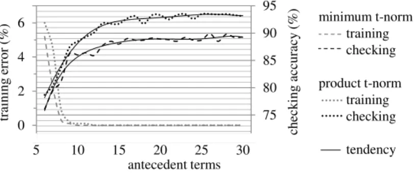
Regarding the FRBCS, to be the focus of the present study, in what follows we approach a more detailed description on the machine learning process, before presenting the accuracy over testing dataset. During the training we found that the gaussian curve membership function afforded a performance better than ones achieved with triangular and trapezoidal-shaped functions. Then, using gaussian functions for the fuzzy partitioning, variations of the number of antecedent terms have been assessed in combination with minimum and product t-norm (Figure 5).
70 75 80 85 90 95 -1 0 1 2 3 4 5 6 7
5 10 15 20 25 30
che ck ing ac cur ac y ( % ) tr ai ni ng er ror ( % ) antecedent terms minimum t-norm training checking product t-norm training checking tendency
Figure 5: Performance of different setings of the fuzzy rule-based classification model, from the variations of the number of antecedent terms in combination with minimum and product t-norm.
that regard, one of the main aspects to highlight is the difference of performance provided by minimum and product t-norm.
Both product and minimum t-norm allowed aggregating the predictor variables via fuzzy inter-sections, modeling the simultaneous occurrence of patterns that characterize the same arboreal species. However, the product t-norm operates multiplying all the membership values and, in con-trast, the minimum t-norm takes into account only the lowest membership during the aggregation process (Figure 6).
x1 x2 x3 x4
R1 φ
R2φ
1 0.64
0
1
0.36 0
1 0.68
0
1
0.32 0
1
0.25 0
1 0.75
0
1
0.30 0 1 0.70
0
p o
p o
X1 X2 X3 X4
min = 0.25; p o = 0.08; min = 0.30; p o = 0.03
Figure 6: Aggregation process of predictor variables (xi) in the
rules 1 (R1) and 2 (R2), using minimum and product t-norm.
In Figure 6 we have a case in which a given sample has features (pattern values) belonging to more than one arboreal species, i.e, a sample with pertinence in both consequent classes of the rules 1 and 2, but with different membership degrees. By using the minimum t-norm the most critical condition given by the lowest membership become decisive, and hence we have a more rigorous classifier, but which can be naive by disregarding the other predictor variables.
As a consequence, for the case in Figure 6 the minimum t-norm would result in the arboreal species identification supported by the rule 2 (ϕmin(R2)>ϕmin(R1)). However, the sample has
higher membership in the majority of the fuzzy regions correspondent to the consequent of the rule 1, as computed by the product t-norm (ϕprod(R1)>ϕprod(R2)). Thus, by taking account all
the predictors, the product t-norm seems to afford a more assertive predictive modeling, so that it provided better performance than minimum t-norm in all settings assessed (see Figure 5).
During the learning process we can note a tendency of accuracy improvement over checking dataset with the increase of the number of fuzzy regions, which was more significant up to about 15 antecedent terms. This improvement seems to occur due to the increase of the decision areas (Dj) formed by each fuzzy if-then rule, as can be seen in Figure 7.
x1 φ x2 x2 x2 φ x1 φ x1 φ Dj 1 0 1 0 1 0 1 0 1 0 1 0 φ φ
Figure 7: Increase in decision areas formed by the fuzzy if-then rules as a consequence of the increment of the number of antecedent terms.
4 CONCLUSIONS
In the present study we analyzed the enforceability of fuzzy-based pattern recognition for dealing with complexity related to the natural variability of texture in the arboreal trunk, which can cause uncertainties due to ambiguity in the pattern matching.
By providing a nonlinear and smooth discriminant function, with the differential of taking into account the graded membership of a given sample in different classes (arboreal species), the Fuzzy Rule-Based Classification System (FRBCS) afforded a high generalization ability, which outperformed the most of assessed learning algorithms, including ensembles with a lot of clas-sifiers and kernel-based models, such as some artificial neural networks, widely used in pattern recognition tasks. Therefore, the fuzzy modeling can be considered an alternative approach, with a competitive and reliable performance for arboreal trunk texture recognition, in order to support the tree species identification using computational intelligence.
ACKNOWLEDGMENTS
Supported by the Coordination for the Improvement of Higher Education Personnel (CAPES).
abor-dagem com desempenho competitivo e confi´avel no reconhecimento da textura em imagens do tronco arb´oreo.
Palavras-chave: computac¸˜ao n˜ao-r´ıgida, processamento de imagens, correspondˆencia de padr˜oes, bioinform´atica.
REFERENCES
[1] S. Abe & R. Thawonmas. A fuzzy classifier with ellipsoidal regions. IEEE Transactions on fuzzy systems,5(3) (1997), 358–368.
[2] V. Adriaenssens, B. De Baets, P.L. Goethals & N. De Pauw. Fuzzy rule-based models for decision support in ecosystem management.Science of the Total Environment,319(1) (2004), 1–12.
[3] C. Arunpriya & A.S. Thanamani. Fuzzy inference system algorithm of plant classification for tea leaf recognition.Indian Journal of Science and Technology,8(S7) (2015), 179–184.
[4] J. Ascough, H. Maier, J. Ravalico & M. Strudley. Future research challenges for incorporation of uncertainty in environmental and ecological decision-making. Ecological modelling,219(3) (2008), 383–399.
[5] E. Bauer & R. Kohavi. An empirical comparison of voting classification algorithms: Bagging, boosting, and variants.Machine learning,36(1-2) (1999), 105–139.
[6] J. Boman.Tree species classification using terrestrial photogrammetry. Master’s thesis, Department of Computing Science, Umea University, Umea (2013).
[7] A. Bressane, J.A. Bagatini, C.H. Biagolini, J.A.F. Roveda, S.R.M.M. Roveda, F.H. Fengler & R.M. Longo. Neuro-fuzzy modeling: a promising alternative for risk analysis in urban afforestation management.Brazilian Journal of Forest Science. IN PRESS.
[8] A. Bressane, C.H. Biagolini, P.S. Mochizuki, J.A.F. Roveda & R.W. Lourenc¸o. Fuzzy-based method-ological proposal for participatory diagnosis in the linear parks management.Ecological Indicators,
80(2017), 153–162.
[9] A. Bressane, P.S. Mochizuki, R.M. Caram & J.A.F. Roveda. A system for evaluating the impact of noise pollution on the population’s health.Reports in public health,32(5) (2016).
[10] A. Bressane, J.A.F. Roveda & A.C. Martins. Statistical analysis of texture in trunk images for biometric identification of tree species. Environmental monitoring and assessment,187(4) (2015), 212.
[11] Z. Chi, H. Yan & T. Pham. Fuzzy algorithms: with applications to image processing and pattern recognition, volume 10. World Scientific (1996).
[12] A.B. Costello & J.W. Osborne. Best practices in exploratory factor analysis: Four recommendations for getting the most from your analysis.Pan-Pacific Management Review,12(2) (2009), 131–146.
[14] R.C. Gonzales & R.E. Woods.Digital image processing, volume 3. Pearson Prentice Hall (2008).
[15] R.C. Gonzales, R.E. Woods & S.L. Eddins. Digital image processing using MATLAB, volume 2. Gatesmark Publishing (2009).
[16] A. Gonzblez & R. P´erez. SLAVE: A genetic learning system based on an iterative approach. IEEE Transactions on Fuzzy Systems,7(2) (1999), 176–191.
[17] R.M. Haralick, K. Shanmugam & I. Dinstein. Textural features for image classification. IEEE Transactions on systems, man, and cybernetics,3(6) (1973), 610–621.
[18] Z.K. Huang. Bark classification using RBPNN based on both color and texture feature.International Journal of Computer Science and Network Security,6(10) (2006), 100–103.
[19] Z.K. Huang, C.H. Zheng, J.X. Du & Y.y. Wan. Bark classification based on textural features using artificial neural networks. In International Symposium on Neural Networks, pp. 355–360. Springer (2006).
[20] H. Ishibuchi & T. Nakashima. Effect of rule weights in fuzzy rule-based classification systems.IEEE Transactions on Fuzzy Systems,9(4) (2001), 506–515.
[21] A. Lermontov, L. Yokoyama, M. Lermontov & M.A.S. Machado. River quality analysis using fuzzy water quality index: Ribeira do Iguape river watershed, Brazil. Ecological Indicators,9(6) (2009), 1188–1197.
[22] D. Liu & Z. Zou. Water quality evaluation based on improved fuzzy matter-element method.Journal of Environmental Sciences,24(7) (2012), 1210–1216.
[23] L. Liu, J. Zhou, X. An, Y. Zhang & L. Yang. Using fuzzy theory and information entropy for water quality assessment in Three Gorges region, China. Expert Systems with Applications,37(3) (2010), 2517–2521.
[24] D. Nauck & R. Kruse. A neuro-fuzzy method to learn fuzzy classification rules from data.Fuzzy sets and Systems,89(3) (1997), 277–288.
[25] W. Pedrycz & F. Gomide.Fuzzy systems engineering: toward human-centric computing. John Wiley & Sons (2007).
[26] A. Porebski, N. Vandenbroucke & L. Macaire. Iterative feature selection for color texture classifica-tion. In Image Processing, 2007. ICIP 2007. IEEE International Conference on, volume 3, pp. III–509. IEEE (2007).
[27] L.S. Riza, C.N. Bergmeir, F. Herrera & J.M. Ben´ıtez S´anchez. frbs: Fuzzy rule-based systems for classification and regression in R.Journal of Statistical Software,65(6) (2015), 1–30.
[28] W. Silvert. Fuzzy indices of environmental conditions. Ecological Modelling,130(1) (2000), 111– 119.
[30] Y.Y. Wan, J.X. Du, D.S. Huang, Z. Chi, Y.M. Cheung, X.F. Wang & G.J. Zhang. Bark texture fea-ture extraction based on statistical texfea-ture analysis. In Intelligent Multimedia, Video and Speech Processing, 2004. Proceedings of 2004 International Symposium on, pp. 482–485. IEEE (2004).
[31] A.G. Yong & S. Pearce. A beginner´s guide to factor analysis: Focusing on exploratory factor analysis.
Tutorials in Quantitative Methods for Psychology,9(2) (2013), 79–94.
[32] L.A. Zadeh. Fuzzy sets.Information and control,8(3) (1965), 338–353.