SOLVING IRREGULAR STRIP PACKING PROBLEMS WITH FREE ROTATIONS USING SEPARATION LINES

(1)

doi: 10.1590/0101-7438.2018.038.02.0195

SOLVING IRREGULAR STRIP PACKING PROBLEMS WITH FREE ROTATIONS USING SEPARATION LINES

Jeinny Peralta

1*

_{, Marina Andretta}

1

_{and Jos´e Fernando Oliveira}

2

Received June 29, 2017 / Accepted March 17, 2018

ABSTRACT.Solving nesting problems or irregular strip packing problems is to position polygons on a fixed width and unlimited length strip, obeying polygon integrity containment constraints and non-overlapping constraints, in order to minimize the used length of the strip. To ensure non-non-overlapping, we use separation lines, i.e., straight lines that separate polygons. We present a nonlinear programming model that considers free rotations of the polygons and of the separation lines. This model uses a considerable smaller number of variables than the few other approaches proposed in the literature. We use the nonlinear programming solver IPOPT (an algorithm of interior points type), which is part of COIN-OR. Computa-tional tests were run using established benchmark instances and the results were compared with the ones obtained with other methodologies in the literature that use free rotations.

Keywords: separation line, irregular packing problems, nonlinear optimization.

1 INTRODUCTION

Irregular strip packing problems have a great relevance in production processes, such as garment, manufacturing and furniture making. In irregular strip packing, smaller irregular pieces (in our case polygons) must be positioned into a big piece (in our case the strip), minimizing the used length of the strip. The main constraint in irregular strip packing problems is the non-overlapping between pieces, but it is very complex for a computational program to determine if two pieces are overlapping, touching or separated. In the literature there are tools for solving this issue (see [5]), among these the raster methods, direct trigonometry, no-fit polygon, and phi-function. In raster methods the strip is always divided into discrete areas and coding schemes are used. In the coding schemes used by Oliveira and Ferreira, and Segenreich and Braga in [22] and [25], respectively, the empty cells belonging to the division of the strip are encoded by zero and numbers equal to

*Corresponding author.

1Instituto de Ciências Matemáticas e de Computação, Universidade de São Paulo, Av.Trabalhador São-carlense, 400, 13566-590 São Carlos, SP, Brasil. E-mails: jeinnyp@icmc.usp.br; andretta@icmc.usp.br

(2)

or greater than one are used to encode a piece; so, to check the non-overlap in raster methods is only a matter of checking the grid cells. There are several tools that use trigonometry to deal with the non-overlapping. In [14] circles inscribed are used to relax the non-overlapping constraints, replacing them with non-overlapping constraints of circles inscribed. In the remaining tools that use trigonometry, the pieces are represented by polygons, thereby the non-intersection of the edges of polygons must be checked to verify the non-overlap. In phi-function, the pieces are represented by the union or intersection of primary objects, that is, circles, rectangles, regular polygons, convex polygons, and the complement of these forms. This tool was designed and implemented in [6, 26, 27, 29]. The phi-function is a mathematical expression that represents the relative position of two pieces. Specifically, the phi-function value is greater than zero if the pieces are separated; equal to zero if their borders are touching; and smaller than zero if overlapping each other. In this article, we use two tools to ensure non-overlapping of pieces, direct trigonometry and no-fit polygon. In the model, we represent the pieces by polygons and use separation lines, that is, we use trigonometry. A straight line is a separation line if given two polygons, all vertices of one of the polygons are on one side of the line or on the line, and all vertices of the other polygon are on the other side of the line or on the line. For the resolution of the modeled problem we need a starting solution; for the construction of this starting solution, we use the no-fit polygon. The no-fit polygon is a polygon resulting from the two polygons that are being compared. One of the advantages of this method is that the generation of these no-fit polygons is done only once, in a pre-processing phase, but a big disadvantage is that the no-fit polygons are dependent on the orientation of the polygons, and have to be generated for all their possible orientations; in all the instances, we use four predefined orientations of the polygons, 0◦,90◦,180◦and 270◦, which is usually done in the literature.

Several solving techniques for these problems that deal with irregular pieces have been devel-oped, based predominantly on heuristics and metaheuristics [1, 10, 13, 17, 20, 22]. The heuristics used for solving these problems can work with partial solutions, constructing the final layout piece by piece (constructive heuristics), or complete solutions, in which changes are done in or-der to find improvements. Exact algorithms based on mixed integer linear programming models that ensure finding the optimal solution were also developed [2, 12, 31]; however, in these algo-rithms, the runtime increases dramatically with the increase of the quantity of objects used in the problem. Few methods that combine exact and heuristic approaches have been developed [9], which allow the computation of high quality solutions in shorter computational times. In all these techniques and algorithms, free rotations are not allowed.

Additionally in the literature, we also find a visual system for packing problem of irregular pieces with free rotation into a rectangular board that aims to minimize the waste [16]. This algorithm is based on Physics, the rubber band physics movement.

(3)

2D and 3D objects of very general type. To solve the problem [8] applied a modification of the Zoutendijk method of feasible directions [34,35] combined with the concept ofǫ-active inequal-ities [28]. In [14] the pieces and the shapes can be arbitrary nonconvex polygons and to solve the problem [14] used three solvers: Branch&Reduce Optimization Navigator (BARON) [24, 30]; the LINDO global optimization procedure (GOP); and The Global Mixed-Integer Quadratic Optimizer (GloMIQO) [18]. In [23], like in [8], a model for an irregular strip packing prob-lem was presented. In this, the resolution of the probprob-lem is divided in two phases: big pieces are compacted in a first phase, while in a second phase, the remaining small pieces are placed between the big pieces. In their experiments, [23] used instances where the pieces are convex and nonconvex irregular polygons. The representation of these polygons was done by circle cov-ering, and they used the nonlinear solver ALGENCAN [3, 4]. In [15] a model for two cases of packing pieces was developed. In the first case, the objective is to pack the pieces in such a way as to minimize the area of the design rectangle. In the second case, the objective is to pack the pieces on stocked rectangles of known geometric dimensions. Separation lines are used to ensure non-overlapping. In their work the pieces are circles, rectangles, and convex polygons; and to solve the problem [15] used BARON [24, 30] and LindoGlobal; an experiment was performed with only two polygons and found a feasible solution for it, in which LindoGlobal proved global optimality in 40 min, but BARON did not increase the lower bound at all. With more than two polygons this technique has difficulty finding an optimal solution to the problem. In [29] it was provided a nonlinear programming model that employs ready-to-use phi-functions. In this paper, the pieces are bounded by circular arcs and/or line segments, and two types of container are con-sidered, rectangular and circular. To solve the problem, [29] developed a compaction algorithm to search for local optimal solutions, which is performed by IPOPT (an algorithm of interior points type, [32]), a component of COIN-OR.

In this paper we propose a nonlinear mathematical model for an irregular strip packing problem which deals only with polygons which may be convex or nonconvex, and that can rotate freely. In the model, to ensure non-overlapping, we use direct trigonometry, in particular separation lines, a similar technique to that used in [15], but with a significantly lower number of variables. The high number of variables in the model used in [15] comes from having all vertices of the polygon as variables. Also, it is due to the line vector equation used to model the separation lines, which in turn implies the employment of many variables such as footing point vector, direction vector, normal vector, vectors connecting the separation line with the vertices, and distance of the vertices to the separation line, among others. In our model only the reference point and the angle of rotation for each polygon and for each separation line are variables, allowing us to obtain good solutions for larger instances in reasonable execution times. Like the polygons, the separation lines also can rotate freely. We use a code for nonlinear programming to solve the problem, IPOPT [32], which depends substantially on a starting solution. We present a way of calculating starting solutions.

(4)

In Section 3, the parameters of the algorithm used for solving the problem are presented, as well as the numerical results obtained when performing tests with known benchmark instances. At the end of our paper we present some conclusions in Section 4.

2 A MODEL FOR AN IRREGULAR STRIP PACKING PROBLEM

The irregular strip packing problem studied in this paper consists of placingnirregular polygons, which can rotate freely, in a fixed width and unlimited length strip, obeying polygon integrity containment constraints and non-overlapping constraints, in order to minimize the used length of the strip. We propose a nonlinear mathematical model for this irregular strip packing problem.

We now explain how the polygons are represented in the model (Section 2.1), as well as the tool used to ensure non-overlapping of the polygons (Section 2.2), and then, introduce the model (Section 2.3).

2.1 Representation of polygons in the model

Here, we describe the representation of the polygons. If a polygon is convex, it is represented by their vertices, as follows:

Pi =(xi1,yi1), (xi2,yi2), . . . , (x

vi

i ,y

vi

i )

,

withvi the number of vertices of the polygonPi.

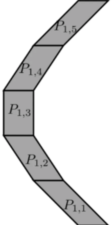
If a polygon is nonconvex, it can be partitioned in convex polygons, as follows:

Pi =Pi,1,Pi,2, . . . ,Pi,pi

,

with pi the number of convex polygons belonging to the partition of the nonconvex polygonPi, see Figure 1.

The partition of a nonconvex polygon influences the model and therefore the solution, because there is a directly proportional relationship between the number of convex polygons belonging to the partition and the number of separation lines. The number of variables and the computational effort will grow according to the number of polygons in the partition.

The coordinates of a vertex belonging to a partition of a nonconvex polygonPi are given by

(xl_i_,_j,y_il_,_j), with j =1, . . . ,pi and l =1, . . . , vi,j,

withvi,j the number of vertices of the convex polygonPi,j.

We can deal with the problem withnnonconvex polygons in the same way that we deal with the problem withNconvex polygons, withN =n

i=1pi. We just have to ensure that the translations and rotations are the same for all polygons belonging to the partition of a nonconvex polygon.

(5)

Figure 1–Partition of a nonconvex polygon.

2.1.1 Vertices of polygons in general form

Henceforth, we will use the following notation:(x_il,yl_i) are the coordinates of a vertex of a polygonPi in the original position, and(x¯li,y¯li)are the coordinates of a vertex of a polygonPi which has undergone translations and/or rotations.

In the representation of the polygons used in the model, we assume that(x_i1,y1_i)=(0,0)for all i. Thus, if we translate and rotate a polygonPiaround its reference point, the coordinates of any vertexlin general form are given by:

¯

x_il,y¯l_i=xl_icosθi −ylisinθi + ¯xi1,xilsinθi+ylicosθi + ¯yi1

,

withθithe angle of rotation of the polygonPi. We consider that positive angles represent rotation in the counterclockwise direction.

When we deal with nonconvex polygons, we make sure that the translations and rotations are the same for all polygons belonging to the partition of the nonconvex polygon.

2.2 Separation lines

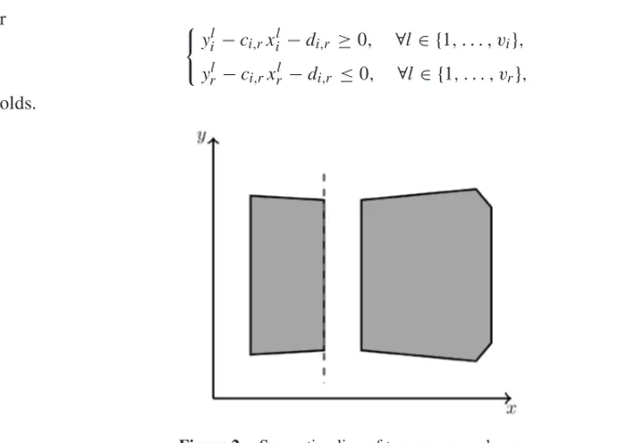
We use separation lines to ensure non-overlapping, see Figure 2. A straight line given by the equationy=ci,rx+di,r separates two polygonsPi andPr if either

yl_i−ci,rxli −di,r ≤0, ∀l∈ {1, . . . , vi}, y_rl −ci,rxrl −di,r ≥0, ∀l ∈ {1, . . . , vr},

(6)

or

y_il−ci,rxil−di,r ≥0, ∀l ∈ {1, . . . , vi}, y_rl −ci,rxrl −di,r ≤0, ∀l∈ {1, . . . , vr},

(2)

holds.

Figure 2–Separation line of two convex polygons.

When we are dealing with nonconvex polygons, we must have lines separating each pair of polygons Pi,j, Pr,s, belonging to the partition of polygons Pi, Pr, respectively, withi = r (that is, we do not have lines separating the polygons belonging to the partition of a nonconvex polygon), j ∈1, . . . ,pi, ands∈1, . . . ,pr.

A separation line does not necessarily pass over one side of one of the two polygons that it is separating; however, at the starting solution, all separation lines have a rotation of 0◦and pass over one side of one of the two polygons that it is separating. Next, we present the general form of a separation line passing through a side of one of the two polygons, that is, which passes through two vertices of a polygon (Pi,j orPr,s), let’s say(xk,yk)and(xk+1,yk+1):

(y−yk)(xk+1−xk)−(yk+1−yk)(x−xk)=0.

Like polygons, the separation lines can also rotate and translate, as long as they remain being sep-aration lines. When rotating and translating a sepsep-aration line, we rewrite the point(x¯k+1,y¯k+1)

as a function of(x¯k,y¯k), which we will call from now on reference point of the separation line; therefore

(x¯k+1,y¯k+1)=((xk+1−xk)cosαi,j,r,s+(yk−yk+1)sinαi,j,r,s + ¯xk, (xk+1−xk)sinαi,j,r,s+(yk+1−yk)cosαi,j,r,s + ¯yk), withαi,j,r,s the angle of rotation of the separation line of the polygonsPi,j andPr,s.

Next, we rewrite the separation line equation:

(7)

2.3 Model for an irregular strip packing problem withnpolygons considering free rotations

Because we want to positionn polygons in a fixed width and unlimited length strip in order to minimize the used length of the strip, the objective function is given by:

z=max{ ¯xil}, l =1,2, . . . , vi and i =1,2, . . . ,n, (3)

withvithe number of vertices of the polygonPi.

Without loss of generality, to ensure non-overlapping, we used in our model the set of con-straints (1), for each pair of polygonsPi,j andPr,s, with

ci,j,r,s =

(xk+1−xk)sinαi,j,r,s +(yk+1−yk)cosαi,j,r,s (xk+1−xk)cosαi,j,r,s +(yk−yk+1)sinαi,j,r,s

and

di,j,r,s = ¯yk−ci,j,r,sx¯k,

in which(xk,yk)and(xk+1,yk+1)are the two vertices of one of the polygons whereby passes

the separation line andαi,j,r,s is the rotation angle of the straight line that separates Pi,j from Pr,s. We use the notation(xk,yk)for the reference point of the separation line. Note that the coordinates of this reference point are also the values of the translations parameters, that from now on, we will write(x¯i,j,r,s,y¯i,j,r,s), for a straight line that is separatingPi,j from Pr,s.

Let (z,q1,q2, . . . ,qn,q¯1,q¯2, . . . ,q¯Q)be the vector of all variables in our model, with z the length of the strip defined in (3),qi the variables referring to the polygonPi,qi =(x¯_i1,y¯1_i, θi), i =1, . . . ,nandq¯ℓthe variables referring to the line that separates polygonPi,j from polygon Pr,s,q¯ℓ=(x¯i,j,r,s,y¯i,j,r,s, αi,j,r,s),ℓ=1, . . . ,QandQ=_in₌−₁1pi(kn=i+1pk)the number of separation lines. Letebe the width of the strip in which the polygons are to be placed. A general model for our problem is given by:

Minimizez

subject to 0≤ ¯yl_i_,_j ≤e, i =1, . . . ,n (4a)

j =1, . . . ,pi

l =1, . . . , vi,j

0≤ ¯xl_i_,_j ≤z, i =1, . . . ,n (4b)

j =1, . . . ,pi

l =1, . . . , vi,j

¯

y_il_,_j −ci,j,r,sx¯il,j −di,j,r,s ≤0,i =1, . . . ,n (4c)

r =1, . . . ,n

i =r

(8)

s=1, . . . ,pr

l=1, . . . , vi,j

¯

y_rl_,_s −ci,j,r,sx¯lr,s −di,j,r,s ≥0,i=1, . . . ,n (4d)

r=1, . . . ,n

i =r

j =1, . . . ,pi

s=1, . . . ,pr

l=1, . . . , vr,s

Remembering that the vertices of a translated and rotated polygonPi,j are given by(x¯il,j,y¯il,j), fori =1, . . . ,n, j =1, . . . ,piandl=1, . . . , vi,j, in which

¯

x_il_,_j =xl_i_,_jcosθi −yil,jsinθi+ ¯xi1,

and

¯

y_il_,_j =xl_i_,_jsinθi+yli,jcosθi+ ¯yi1,

with (x¯_i1,y¯1_i) the variable reference point of polygon Pi and θi the variable rotation angle. (x_il_,_j,yl_i_,_j)are the coordinates of a vertex of a polygonPiin the original position.

Constraints (4a) and (4b) ensure that a polygonPiis entirely inside the strip. In these constraints, the widtheis a fixed parameter; the lengthzis a variable;x¯l_i_,_j andy¯_il_,_j depend on the reference point and the rotation angle of the polygon,(x¯_i1,y¯_i1)andθi, respectively, which are variables. Constraints (4c) and (4d) ensure non-overlapping of the convex polygonsPi,j andPr,s. In these constraints,ci,j,r,s anddi,j,r,s depend on the reference point and the rotation angle of the separa-tion line,(x¯i,j,r,s,y¯i,j,r,s)andαi,j,r,s, respectively, which are variables.

3 COMPUTATIONAL EXPERIMENTS AND RESULTS

All numerical experiments were performed on an Intel Core I7-4510U CPU @ 2.1GHz processor and 8 GB of memory. We used a code for nonlinear programming to solve the problem, IPOPT [32] (an algorithm of interior points type), which is part of the COIN-OR [33].

IPOPT is the implementation of a barrier or interior points method for large scale nonlinear optimization problems of the type

Minimize f(v) subject to gL ≤ g(v)≤gU,

vL ≤ v≤vU,

(9)

C programming language version of Ipopt-3.12.3 and compiled the codes in the Ubuntu 12.04 operating system.

The CPU time is very large when we use the Hessian of the Lagrangian, therefore we will always use an option given in IPOPT to approximate the Hessian with limited memory, which makes the runtime shorter, without affecting the quality of the solution. In addition to the standard IPOPT parameters, we use the adaptive update strategy for barrier parameter. The maximum execution time is set to one hour.

We use the geometric library Computational Geometry Algorithms Library (CGAL) to partition the nonconvex polygons, in particular, we use the implementation of Greene’s dynamic program-ming algorithm [7].

In the next subsection a brief explanation of the starting solution used in the execution of IPOPT is presented. In Section 3.2, the results obtained with IPOPT and comparisons of those with two methodologies recent in the literature [16, 29], which also allow free rotations, are presented.

3.1 Starting solutions

IPOPT is designed to find local solutions. Taking into account that the developed nonlinear model is nonconvex, when solving it we can find many stationary points with different objective func-tion values, and these stafunc-tionary points depend on the starting solufunc-tion.

In the next section we present the instances that are used to test our model. For each one of these instances, we generate a starting solution using a bottom-left algorithm. The bottom-left algorithm is a single pass heuristic that, given a set of pieces and an order, places the pieces one by one on the strip, as far to the left and to the bottom as possible. The algorithm receives a list of randomly ordered polygons. This list is represented by a sequence, and for decoding the sequences, we used the technique presented in [19]. To avoid overlapping, the algorithm uses no-fit raster, concept also introduced in [19]. In no-fit raster, to represent the strip a discrete grid of points is used. The scale used for discretization in most instances is 1.0, except for Albano, Dagli, and Swim, (instances in which the area occupied by the polygons is greater), which are 0.02, 0.5, and 0.00005, respectively. Although in the model we allow free rotation, this bottom-left algorithm does not allow free rotation of the polygons, therefore we use four predefined angles of rotation (0◦,90◦,180◦and 270◦) in all instances. For each instance, we execute the algorithm 1000 times, then we choose the layout with shortest length obtained from these 1000 executions as a starting solution.

3.2 Comparing results

(10)

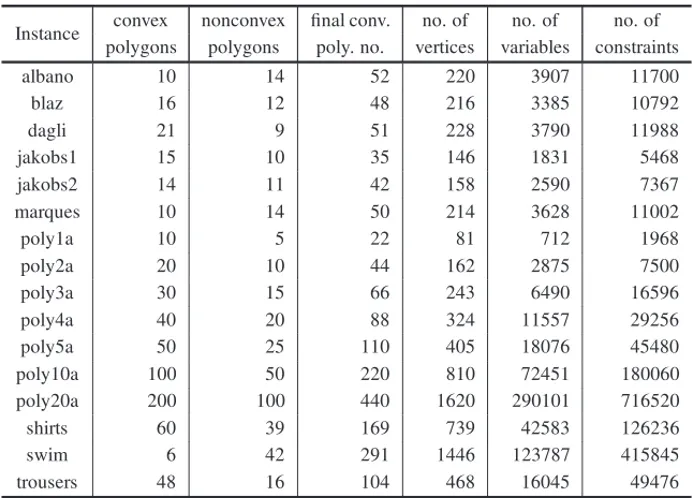
convex polygons are presented in the fourth column. In the fifth the total number of vertices are presented. The number of variables and the number of constraints are presented in the sixth and seventh columns, respectively.

Table 1–Instances data.

Instance convex nonconvex final conv. no. of no. of no. of

polygons polygons poly. no. vertices variables constraints

albano 10 14 52 220 3907 11700

blaz 16 12 48 216 3385 10792

dagli 21 9 51 228 3790 11988

jakobs1 15 10 35 146 1831 5468

jakobs2 14 11 42 158 2590 7367

marques 10 14 50 214 3628 11002

poly1a 10 5 22 81 712 1968

poly2a 20 10 44 162 2875 7500

poly3a 30 15 66 243 6490 16596

poly4a 40 20 88 324 11557 29256

poly5a 50 25 110 405 18076 45480

poly10a 100 50 220 810 72451 180060

poly20a 200 100 440 1620 290101 716520

shirts 60 39 169 739 42583 126236

swim 6 42 291 1446 123787 415845

trousers 48 16 104 468 16045 49476

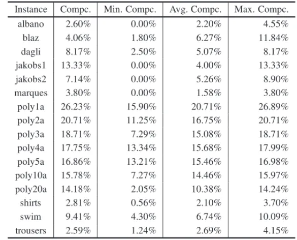
A starting solution is the layout with shortest length, among 1000 executions of the bottom-left algorithm applied to random piece sequences. As the sequence of the polygons is random, if we execute the algorithm another 1000 times, the layout with shortest length can be different to the one found previously, thus, in order to analyze the effectiveness of our model, for each instance, we considered 10 starting solutions. We execute IPOPT to solve our model with each one of these 10 different starting solutions.

(11)

Table 2–Compaction percentages from length in the starting solution to length in the solution.

Instance Compc. Min. Compc. Avg. Compc. Max. Compc.

albano 2.60% 0.00% 2.20% 4.55%

blaz 4.06% 1.80% 6.27% 11.84%

dagli 8.17% 2.50% 5.07% 8.17%

jakobs1 13.33% 0.00% 4.00% 13.33%

jakobs2 7.14% 0.00% 5.26% 8.90%

marques 3.80% 0.00% 1.58% 3.80%

poly1a 26.23% 15.90% 20.71% 26.89%

poly2a 20.71% 11.25% 16.75% 20.71%

poly3a 18.71% 7.29% 15.08% 18.71%

poly4a 17.75% 13.34% 15.68% 17.99%

poly5a 16.86% 13.21% 15.46% 16.98%

poly10a 15.78% 7.27% 14.46% 15.97%

poly20a 14.18% 2.05% 10.38% 14.24%

shirts 2.81% 0.56% 2.10% 3.70%

swim 9.41% 4.30% 6.74% 10.09%

trousers 2.59% 1.24% 2.69% 4.15%

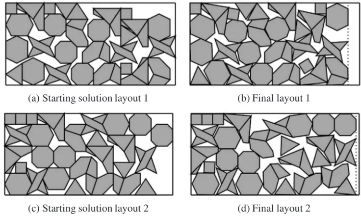
The length of the starting solution does not have a determinant impact on the length of the solution, the layout of the starting solution is what determines the length of the solution; two starting solutions with the same length can produce two solutions with quite different lengths, as long as the layouts at the starting solutions are enough different, see Figure 3. In our experiments, we have observed that in 10 of the 16 instances tested the shortest starting solution produced the shortest solution.

We solved the model in Section 2.3 for the instances of Table 1 using the 10 different starting solutions and we compared our results with those of the recent literature that allow free rota-tions, [29] and [16]. These results are summarized in Table 3, in which the minimum (second column), the average (third column), and the maximum (fourth column) strip length obtained are presented. The average time used to construct the starting solutions (fifth column) and the average time (sixth column) that was spent to solve the instances are also presented in Table 3 ; the strip length and time reported in [29] are in seventh and eighth columns, and strip length and time reported in [16] are in ninth and tenth columns, respectively.

(12)

(a) Starting solution layout 1 (b) Final layout 1

(c) Starting solution layout 2 (d) Final layout 2

Figure 3–Example of two starting solutions with the same length and solutions with quite different lengths.

Table 3–Comparison of our results to those in [29] and [16].

Instance

Our approach Best results in [29] Best results in [16] Minimal

Solution Average Solution

Maximal Solution

SP Average time(sec)

IPOPT Average

time(sec) Length Time(sec) Length Time(sec) albano 10355.80 10601.03 10849.99 158.68 178.56 10032.24 124.39

blaz 27.82 29.02 30.44 1.37 49.52 25.41 25.42 28.27 56.86

dagli 60.60 61.96 63.36 404.13 135.10 56.90 139.00 59.24 132.58

jakobs1 12.99 13.49 14.00 4.68 19.30 13.19 48.46

jakobs2 26.00 27.29 30.00 17.60 18.41 24.25 53.67

marques 84.65 86.68 91.00 66.74 58.11 84.93 118.12

poly1a 14.01 14.53 15.01 6.23 19.07 13.90 27.59

poly2a 26.16 27.30 27.92 10.68 87.53 26.67 61.23

poly3a 39.01 40.29 44.50 15.44 773.32 39.48 149.66

poly4a 50.99 52.50 53.72 20.59 1621.54 51.13 210.74

poly5a 63.66 65.05 66.31 26.21 1773.85 65.64 287.32

poly10a 127.16 129.46 140.01 58.25 2350.17 126.29 618.80 poly20a 254.86 268.06 294.81 151.38 3484.92 251.04 1209.17

shirts 62.19 64.43 65.62 11.55 1808.73 65.06 340.89

swim 6011.93 6311.16 6526.38 449.85 3600.00 5661.95 431.97

trousers 249.35 258.03 261.94 118.00 603.36 251.94 265.48

(13)

(a) Starting solution layout (b) Final layout

Figure 4–Instance Albano.

Figure 5–Instance Blaz.

Figure 6–Instance Dagli.

(14)

Figure 8–Instance Jakobs2.

Figure 9–Instance Marques.

Figure 10–Instance Poly1a.

4 CONCLUSIONS

(15)

(16)

(a) Starting solution layout

(b) Final layout

(17)

Figure 18–Instance Swim.

(b) Final layout

Figure 19–Instance Trousers.

vector equation of the line used to model the separation line. In fact, a instance with two convex polygons of 5 and 6 vertices would use:

• For the separation lines: eleven variables for the distances of the vertices to the sepa-ration line, two variables for the footing point vector, twenty two variables for the vec-tors connecting the separation line with the vertices, eleven auxiliary variables needed to compute these vectors, two variables for the direction vector and, two variables for the normal vector.

• For the polygons: two variables for the orientation angle of the polygons, two variables for the radius of the smallest circle enclosing the polygons, twenty two variables for the coordinates of the vertices and, four variables for the center coordinates of the polygons.

(18)

Instead, for an instance with two convex polygons our model would only need 10 variables, a significant simplification that leads to a better performance of the solution method ensuring likewise a good solution to the problem.

The solution of the problem modeled here, using a local nonlinear programming solver, depends on the starting solution. We used a bottom-left algorithm to construct these starting solutions. To test the effectiveness of our model, we compared our results with those obtained recently in the literature [16, 29], which also use methodologies with free rotations. The lengths reported in [29] are smaller but very close to those found in this work. On the other hand, the lengths reported in [16] are greater in most instances; in the others, they are very close. Therefore, the effectiveness of our model is verified, as well as the quality of the constructed starting solutions using a bottom-left algorithm; however, we believe that these results could be improved by using another algorithm to construct the starting solutions.

ACKNOWLEDGEMENTS

This research was partially supported by CNPq (grants 141072/2014-8 and 409043/2016-8) and FAPESP (grants 2013/07375-0 and 2016/01860-1), from Brazil.

REFERENCES

[1] ALBANO A & SAPUPPOA. 1980. Optimal allocation of two-dimensional irregular shapes using heuristic search methods.IEEE Transactions on Systems, Man and Cybernetics,10: 242–248. [2] ALVAREZ-VALDESR, MARTINEZA & TAMARITJM. 2013. A branch and bound algorithm for

cutting and packing irregularly shaped pieces. International Journal of Production Economics,

145(2): 463–477.

[3] ANDREANIR, BIRGINEG, MARTINEZJM & SCHUVERDTML. 2007. On augmented lagrangian methods with general lower-level constraints.SIAM Journal on Optimization,18: 1286–1309. [4] ANDREANI R, BIRGINEG, MARTINEZ JM & SCHUVERDTML. 2008. Augmented lagrangian

methods under the Constant Positive Linear Dependence constraint qualification. Mathematical Programming,111: 5–32.

[5] BENNELLJA & OLIVEIRAJF. 2008. The geometry of nesting problems: A tutorial.European Jour-nal of OperatioJour-nal Research,184: 397–415.

[6] BENNELL JA, SCHEITHAUER G, STOYAN Y & ROMANOVAT. 2010. Tools of mathematical modelling of arbitrary object packing problems.Ann. Oper. Res.,179: 343–368.

[7] CGAL – COMPUTATIONALGEOMETRYALGORITHMSLIBRARY. 2D Polygon Partitioning.

Avail-able at:http://doc.cgal.org/latest/Partition_2/

[8] CHERNOVN, STOYANY & ROMANOVAT. 2010. Mathematical model and efficient algorithms for object packing problem.Computational Geometry: Theory and Applications,43: 535–553. [9] CHERRIL, CARRAVILLAM & TOLEDOF. 2016. A model-based heuristic for the irregular strip

(19)

[10] EGEBLAD J, NIELSENBK & ODGAARDA. 2007. Fast neighborhood search for two and three-dimensional nesting problems.European Journal of Operational Research,183: 1294–1266. [11] EURO SPECIALINTERESTGROUP ONCUTTING ANDPACKING. 2015. Available at: http://

paginas.fe.up.pt/˜esicup/datasets

[12] FISCHETTIM & LUZZII. 2009. Mixed-integer programming models for nesting problems.Journal of Heuristics,15(3): 201–226.

[13] GOMESAM & OLIVEIRAJF. 2002. A 2-exchange heuristic for nesting problems.European Journal of Operational Research,141: 359–370.

[14] JONESDR. 2013. A fully general, exact algorithm for nesting irregular shapes.Journal of Global Optimization,59: 367–404.

[15] KALLRATH J. 2009. Cutting circles and polygons from area-minimizing rectangles. Journal of Global Optimization,43: 299–328.

[16] LIAOX, MAJ, OUC, LONGF & LIUX. 2016. Visual nesting system for irregular cutting-stock problem based on rubber band packing algorithm.Advances in Mechanical Engineering,8(6): 1–15. [17] MARQUESVM, BISPOCF & SENTIEIROJJ. 1991. A system for the compaction of two-dimensional irregular shapes based on simulated annealing.IEEE Transactions on Industrial Electronics, Control and Instrumentation,3: 1911–1916.

[18] MISENERR & FLOUDASCA. 2013. GloMIQO: global mixed-integer quadratic optimizer.Journal Global Optimization,57: 3–50.

[19] MUNDIMLR, ANDRETTAM & QUEIROZTA. 2017. A biased random key genetic algorithm for open dimension nesting problems using no-fit raster.Expert Systems with Applications,81: 358–371. [20] NIELSENBK. 2007. An efficient solution method for relaxed variants of the nesting problem.

Pro-ceedings of the thirteenth Australasian symposium on Theory of computing,65: 123–130.

[21] NOCEDALJ, W ¨ACHTERA & WALTZRA. 2009. Adaptive barrier strategies for nonlinear interior methods.SIAM Journal on Optimization,19: 1674–1693.

[22] OLIVEIRAJF & FERREIRAJS. 1993. Algorithms for nesting problems Applied simulated annealing, In: VIDALRVV. (Ed.),Lecture notes in econ. and Maths Systems. Springer Verlag,396: 255–274. [23] ROCHAP, RODRIGUESR, GOMESAM, TOLEDOFMB & ANDRETTAM. 2015. Two-Phase

Ap-proach to the Nesting problem with continuous rotations.IFAC-PapersOnline,48(3): 501–506. [24] SAHINIDIS NV. 2014. BARON 14.3.1: Global Optimization of Mixed-Integer Nonlinear

Pro-grams.User’s Manual. Available at: http://www.minlp.com/downloads/docs/baron\ %20manual.pdf

[25] SEGENREICHSA & BRAGALM. 1986. Optimal nesting of general plane figures: a Monte Carlo heuristical approach.Computers and Graphics,10: 229–237.

[26] STOYANYG, TERNOJ, SCHEITHAUERG, GILN & ROMANOVAT. 2001. Phi-functions for primary 2d-objects.Studia Informatica Universalis,2(1): 1–32.

(20)

[28] STOYANYG & CHUGAYAM. 2008. Packing cylinders and rectangular parallelepipeds with dis-tances between them.European Journal Operation Research,197: 446–455.

[29] STOYANYG, PANKRATOVA & ROMANOVAT. 2016. Cutting and packing problems for irregular objects with continuous rotations: mathematical modelling and non-linear optimization.Journal of the Operational Research Society,67(5): 786–800.

[30] TAWARMALANIM & SAHINIDISNV. 2005. A polyhedral brach-and-cut approach to global opti-mization.Mathematical Programming,103(2): 225–249.

[31] TOLEDOFMB, CARRAVILLAMA, RIBEIROC, OLIVEIRAJF & GOMESAM. 2013. The dotted-board model: A new mip model for nesting irregular shapes.International Journal of Production Economics,145(2): 478–487.

[32] W ¨ACHTERA & BIEGLERLT. 2006. On the implementation of a primal-dual interior point filter line search algorithm for large-scale nonlinear programming.Mathematical Programming,106(1): 25–57.

[33] W ¨ACHTER A & BIEGLER LT. 2015. COIN OR project, Available at: http://projects. coin-or.org/Ipopt

[34] ZOUTENDIJKG. 1960. Methods of feasible directions, a study in linear and non-linear programming, Elsevier.