Integrating packing and distribution problems and optimization through mathematical programming

(1)

* Corresponding author.

Contents lists available at GrowingScience

Decision Science Letters

homepage: www.GrowingScience.com/dsl

Integrating packing and distribution problems and optimization through

mathematical programming

Fabio Miguela_{, Mariano Frutos}b*_{, Fernando Tohmé}c_{and Máximo Méndez}d

a_{Sede Alto Valle y Valle Medio, Universidad Nacional de Río Negro. Tacuarí 669, Villa Regina, Argentina}

b_{Department of Engineering, Universidad Nacional del Sur and IIESS-CONICET. Avda. Alem 1253, Bahía Blanca, Argentina} c_{Department of Economics, Universidad Nacional del Sur and INMABB-CONICET. 12 de Octubre 1198, Bahía Blanca, Argentina}

d_{Instituto Universitario de Sistemas Inteligentes y Aplicaciones Numéricas en Ingeniería (SIANI), Universidad de Las Palmas de Gran Canaria (ULPGC).}

Campus Universitario de Tafira, 35017 Las Palmas de Gran Canaria, Spain

C H R O N I C L E A B S T R A C T

Article history: Received June 25, 2015 Received in revised format: October 12, 2015 Accepted October 22, 2015 Available online October 24 2015

This paper analyzes the integration of two combinatorial problems that frequently arise in production and distribution systems. One is the Bin Packing Problem (BPP) problem, which involves finding an ordering of some objects of different volumes to be packed into the minimal number of containers of the same or different size. An optimal solution to this NP-Hard problem can be approximated by means of meta-heuristic methods. On the other hand, we consider the Capacitated Vehicle Routing Problem with Time Windows (CVRPTW), which is a variant of the Travelling Salesman Problem (again a NP-Hard problem) with extra constraints. Here we model those two problems in a single framework and use an evolutionary meta-heuristics to solve them jointly. Furthermore, we use data from a real world company as a test-bed for the method introduced here.

Bin packing problem Capacitated vehicle routing problem with time windows Logistics

Optimization

1. Introduction

(2)

318

approximately optimal solutions. The combination of both problems involves, given a set of requests of several customers, vehicles and routes serving them in an efficient way. We have to determine what requests can be satisfied by the same vehicle in such a way as to use efficiently its capacity, reducing the costs of distribution. Before analyzing the joint problem we will briefly discuss each of the problems separately.

1.1 The Vehicle Routing Problem

Given a class of vehicles and two groups, one of customers and the other of depots, both distributed geographically, the Vehicle Routing Problem requires finding minimal cost routes starting and ending at the depots such the vehicles visit each customer at most once (Frutos & Tohmé, 2012; Escobaret al., 2014; Oyola & Løkketangen, 2014). The solution depends on several parameters, namely the size of the vehicle fleet, the degree of heterogeneity and capacity of the vehicles, the number of depots, the degree of randomness of the demand, the time windows of the service, etc. Each selection yields a different setting, of which the most basic one is the Traveling Salesman Problem (TSP), which provides a ground on which more complicated and practical instances can be stated (Theys et al., 2010). In the TSP a sole vehicle has to visit each customer on a single, minimal cost route. That is, the total distance covered by the vehicle should be minimal. The complexity of this problem stems from the fact that in a general and symmetric case with n customers the number of feasible routes is



n 1 ! 2



. It is easy to see that this problem belongs to the NP-complete class.

TSP can be extended to the multiple TSP (m-TSP), m salesmen have to cover a determinate number of cities, such that each one is visited by only one of the agents. Each route is a round trip starting on a given base-city. The goal here is minimize the total distance covered by the different vehicles. In turn, the Vehicle Routing Problem (VRP) generalizes m-TSP adding a customer-specific demand; geographically distributed depots and a vehicle-specific capacity (Kallehauge et al., 2006) (Fig. 1). With the additional requirement that the total demand on a route cannot exceed the capacity of the corresponding vehicle we get the Capacitated Vehicle Routing Problem (CVRP) (Frutos & Tohmé, 2012; Kao et al., 2013; Sitek, 2014).

Fig. 1. Solution to a VRP problem with three vehicles and a single depot

(3)

each customer is visited by just one vehicle, (iii) the total demand on a route does not exceed the capacity of the vehicle serving it, (iv) the departure and arrival times at the depot fall inside a given time window, and (v) the total cost (distance plus the penalties for violating the time windows of the customers) are minimal.

1.2 The Bin Packing Problem

The Bin Packing Problem (BPP) is that of packing a set of objects in several containers such that the total weight or volume does not surpass the capacity of the container, minimizing the number and the cost of use of containers (Baumgartner et al., 2011; Bennell et al., 2013). Many real world packing problems can be modeled as instances of the BPP, like the determination of the optimal amount to load in trucks and other vehicles (Lodi et al., 2012).

2. The Combined Problem

If capacity is measured only on a single dimension, the problem of loading and distributing cargo in a fleet of vehicles would be represented by CVRPTW (Bräysy, 2003). But real world goods have several features each of which corresponds to a dimension of capacity, e.g. weight; surface of the floor of the container; volume of the container; fragility (which determines if it can be piled) etc. (Iori et al., 2007). So, the goal is, on one hand, to optimally pack a bunch of elements in a set of containers with given dimensions. On the other, the packing must be done such that each vehicle serves the customers on a route. Separate optimal solutions to the packing and routing problems can yield a joint sub-optimal solution. Thus, it is convenient to integrate the problems in a single framework as to capture the interdependences among the problems (Fig. 2).

Fig. 2. Joint BPP and CVRP setting

2.1 Parameters of the Model

CVRPTW is defined on a graph G



V, A



, where the class of nodes is V



0, n 1

 

 1,..., n



, where

(4)

320

iC is a class P_i of items with total weight q_i, to be satisfied by a vehicle in a service time s_i. Each item h  P has width f_h and height e_h, where P i C Pi. Associated to each i there is a time window



a , bi i



of delivery. A vehicle arriving before a_i has to wait until the time window opens, while if delivering after

i

b is penalized by an amount L i

c . For the deposit node we assume q_0,p q_{n 1,p} s₀s_{n 1} 0. The time

window for this node (being a₀a_{n 1}_, b₀b_{n 1}_ ) represents the overall departure and arrival time of the vehicles. The fleet consists of m identical vehicles of capacity Q (indexed by K



1,..., m



). Each vehicle may cover at most one route and cannot split the deliveries to any customer, thus being forced to visit each customer only once. Each vehicle has a rectangular load space of width k

f and height k

e . Items have a fixed orientation and have to be packed in parallel to the borders of the floor of the vehicles. Furthermore, they cannot be rotated.

2.2 The Variables and Constraints of the Problem

The binary variable xijk has value 1 iff vehicle kK goes through edge

 

i, j A. Another binary

variable y_ik is 1 iff customer iV is visited by vehicle k (both binary variables are 0 otherwise). Temporal variable w_ik represents the moment in which vehicle k starts serving customer i. The decision variable u_i indicates the delay in the service to i. Variable v_hk is 1 if item h is loaded on vehicle k and 0 otherwise. Variable z_hl is 1 if items h and l are loaded together and 0 otherwise. To avoid superposition, L

hl

o will be 1 iff item l is laid on the left of h. On the other hand, U hl

o will be 1 iff item l

is below item h, to avoid vertical superposition. M are large constants. X h

c and Y h

c indicate the plane coordinates (x,y) of the lower left corner of item h. Finally, F

k

c is the cost of vehicle k. Then, expressions (1-26) represent the entire model:





F L

k 0,n 1,k ij ijk i i

k K i V j V k K i V

min c 1 x  c x c u

    

   



 



(1)

s.t.

ip ik i V p P

q y Q, k K

 

  



(2)



ijk jk j V

x y , i V \ n 1 , k K



    



(6)

ik i ij ij ijk

w   s t w M(1 x ), i, j  V, kK (7)

i ik i i

k K

a w b u , i C







    (8)





i ik i i

a w b u , k K, i 0, n 1 (9)

 

ijk

x  0,1 , i, j V, kK (10)

 

ik

y  0,1 , i V, kK (11)

ik

w   0, i V, kK (12)

i

u   0, i V (13)

hk k K

v 1, h P



  

(5)

ik hk i

y v , k K, iC, hP (15)

X P K

h h

c f f , h P (16)

ik 0,n 1,k

i C

y M 1 x _ , k K



   



(22)

L L U U

hl lh hl lh

o o o o  1, h, lP (23)

X Y

h h

c , c   0, h P (24)

 

L U

hl hl hl

z , o , o ,0,1 , h, l P  (25)

 

hk

v  0,1 , h P, kK (26)

Eq. (1) states the goal, namely the minimization of total cost. Eq. (2) is the per-vehicle capacity constraint. Eqs. (3-4) ensure that each customer is visited only once and the depot is used by all the vehicles. Flow conservation is ensured by Eqs. (5-6), while Eq. (7) warrants the satisfaction of time constraints. Expressions (8,9) enforce the time windows whose violations are penalized in the objective function. Eqs. (10-13) specify the domains of some variables. Constraints (14,15), combined with Eq. (3) indicate that all items have to be loaded in vehicles and that all items P_i corresponding to customer i must be consolidated in a single vehicle k. Eqs. (16-17) mandate that no items can be loaded as to exceed the perimeter constraints of the vehicles. In turn, constraints (18-21) ensure that no items can be superposed (instead of piled up) in vehicle k. Inequality (22) ensures that only vehicles in use can be loaded. Finally, Eqs. (23-26) impose conditions on the rest of the variables.

3. An Instance of the Problem and its Solution

To run the model on a real-world case we have chosen data from a fruit company in Rio Negro (Argentina) and its provision area in Buenos Aires. This company has a depot in the city (N1) and 3

refrigerated vehicles with the same load capacity, intended to cater its customers in 10 marketplaces across Buenos Aires.

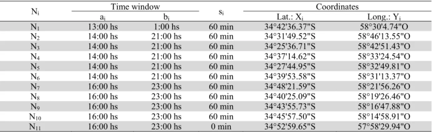
Table 1

Customer nodes

Ni Time window si Coordinates

ai bi Lat.: Xi Long.: Yi

N1 13:00 hs 1:00 hs 60 min 34°42'36.37"S 58°30'4.74"O

N2 14:00 hs 21:00 hs 60 min 34°31'49.52"S 58°46'13.55"O

N3 14:00 hs 21:00 hs 60 min 34°25'36.71"S 58°42'51.43"O

N4 14:00 hs 21:00 hs 60 min 34°37'14.62"S 58°33'24.54"O

N5 14:00 hs 21:00 hs 60 min 34°27'44.95"S 58°32'49.81"O

N6 14:00 hs 21:00 hs 60 min 34°39'53.58"S 58°31'13.37"O

N7 16:00 hs 23:00 hs 60 min 34°48'21.59"S 58°21'56.26"O

N8 16:00 hs 23:00 hs 60 min 34°40'25.09"S 58°19'26.46"O

N9 16:00 hs 23:00 hs 60 min 34°43'55.73"S 58°16'47.88"O

N10 16:00 hs 23:00 hs 60 min 34°45'57.50"S 58°14'58.91"O

(6)

322

Table 1 specifies these markets (Ni, i = 1,…,11, where N1 is the depot) and their corresponding time

windows are (ai,bi), i = 1,…,11. We also specify the servicing time si for each customer as well as its

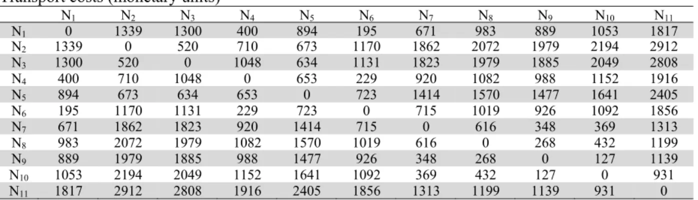
corresponding geographical position (Latitude: Xi, Longitude: Yi). Table 2 specifies the transport costs

ij

c while Table 3 the travel times tij, for each pair of customers (i,j). As said, the fleet based on node

N1 has m=3 refrigerated vehicles, each one with a capacity Qk=26.000 Kg. The rectangular loading

space has dimensions fk_{= 2.5 m and e}k_{=13.5 m (i.e. a floor surface of 33.75 m}2_{). The demand of each}

customerN | i_i 2,...,11, consists of a number Pi of pallets of apples o pears. Each item hPi is a pallet

of width fh=1.2 m and length eh=1.0. The weight of the demand of customer i is the sum of the weights

of all the requested pallets.

Table 2

Transport costs (monetary units)

N1 N2 N3 N4 N5 N6 N7 N8 N9 N10 N11

N1 0 1339 1300 400 894 195 671 983 889 1053 1817

N2 1339 0 520 710 673 1170 1862 2072 1979 2194 2912

N3 1300 520 0 1048 634 1131 1823 1979 1885 2049 2808

N4 400 710 1048 0 653 229 920 1082 988 1152 1916

N5 894 673 634 653 0 723 1414 1570 1477 1641 2405

N6 195 1170 1131 229 723 0 715 1019 926 1092 1856

N7 671 1862 1823 920 1414 715 0 616 348 369 1313

N8 983 2072 1979 1082 1570 1019 616 0 268 432 1199

N9 889 1979 1885 988 1477 926 348 268 0 127 1139

N10 1053 2194 2049 1152 1641 1092 369 432 127 0 931

N11 1817 2912 2808 1916 2405 1856 1313 1199 1139 931 0

The weight of an apple pallet is happle=994.70 Kg while the corresponding to a pear one is hpear=1.136.80

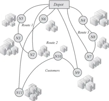
Kg. Each customer formulates its demand according to the stocks available in the depot. A failure in delivering the demanded pallets means that the customer marketplace will be left out of stock. The trucks are loaded under a LIFO (last in first out) policy and the optimization goal is to load the vehicles such that they are able to deliver all the demanded pallets to the customers on their corresponding routes. Fig. 3 shows the graph of the problem. It has 11 nodes and 110 edges.

Table 3

Travel times (minutes)

N1 N2 N3 N4 N5 N6 N7 N8 N9 N10 N11

N1 0 134 112 50 84 25 103 84 100 126 134

N2 134 0 75 126 95 126 221 182 198 224 232

N3 112 75 0 106 72 103 198 162 179 204 212

N4 50 126 106 0 81 42 137 100 117 142 151

N5 84 95 72 81 0 75 170 134 151 176 184

N6 25 126 103 42 75 0 112 92 109 131 140

N7 103 221 198 137 170 112 0 117 81 72 156

N8 84 182 162 100 134 92 117 0 53 78 89

N9 100 198 179 117 151 109 81 53 0 36 100

N10 126 224 204 142 176 131 72 78 36 0 98

N11 134 232 212 151 184 140 156 89 100 98 0

(7)

Fig. 3. Graph of the routing problem

4 Results

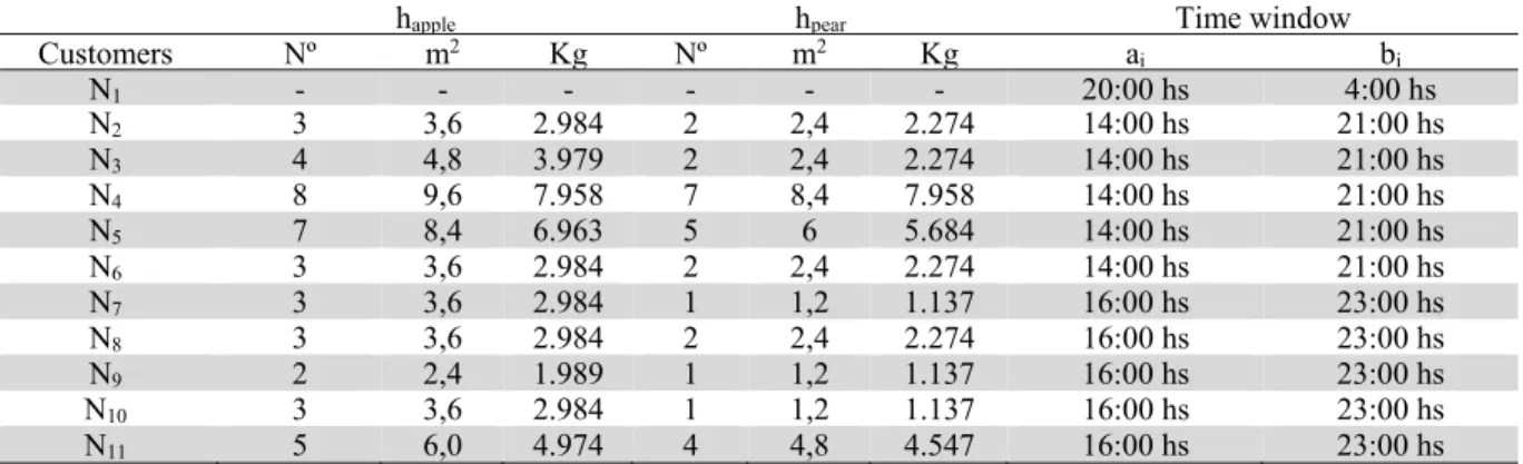
We considered the demands reported on Table 4, and compared the outcomes under our procedure to the real-world actions taken by the company.

Table 4

Demands

happle hpear Time window

Customers Nº m2 _Kg _Nº _m2 _Kg _a

i bi

N1 - - - - - - 20:00 hs 4:00 hs

N2 3 3,6 2.984 2 2,4 2.274 14:00 hs 21:00 hs

N3 4 4,8 3.979 2 2,4 2.274 14:00 hs 21:00 hs

N4 8 9,6 7.958 7 8,4 7.958 14:00 hs 21:00 hs

N5 7 8,4 6.963 5 6 5.684 14:00 hs 21:00 hs

N6 3 3,6 2.984 2 2,4 2.274 14:00 hs 21:00 hs

N7 3 3,6 2.984 1 1,2 1.137 16:00 hs 23:00 hs

N8 3 3,6 2.984 2 2,4 2.274 16:00 hs 23:00 hs

N9 2 2,4 1.989 1 1,2 1.137 16:00 hs 23:00 hs

N10 3 3,6 2.984 1 1,2 1.137 16:00 hs 23:00 hs

N11 5 6,0 4.974 4 4,8 4.547 16:00 hs 23:00 hs

In the real world, the company underused the vehicles: in average each truck was loaded only up to a 70% of its capacity.

(8)

324

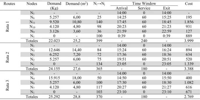
Furthermore, to reach the time windows, they frequently rented an extra truck, increasing the overall costs of the operation. In other cases the company just missed the deadlines, having thus to pay penalties. Our integrated method improved substantially these outcomes. Fig. 4 presents a directed graph summarizing the solution while Table 5 presents the solutions.

Table 5 Solutions

Routes Nodes Demand (Kg)

Demand (m2₎ _N

i→Nj Time Window Cost

Arrival Service Exit

Ruta 1

N1 - - - 14:00 0 14:00

-N6 5.257 6,00 25 14:25 60 15:25 195

N11 9.520 10,80 140 17:45 60 18:45 1.856

N10 4.120 4,80 98 20:23 60 21:23 931

N9 3.126 3,60 36 21:59 60 22:59 127

N1 0 - 100 0:39 0 0:39 889

Totales 22.023 25,2 399 - 240 - 3.999

Ruta 2

N1 - - - 14:00 0 14:00

-N5 12.646 14,40 84 15:24 60 16:24 894

N3 6.252 7,20 72 17:36 60 18:36 634

N2 5.257 6,00 75 19:51 60 20:51 520

N1 0 - 134 23:05 0 23:05 1.339

Totales 24.155 27,6 365 - 180 - 3.388

Ruta 3

N1 - - - 14:00 0 14:00

-N4 15.915 18,00 50 14:50 60 15:50 400

N8 5.257 6,00 100 17:30 60 18:30 1.082

N7 4.120 4,80 117 20:27 60 21:27 616

N1 0 - 103 23:10 0 23:10 671

Totales 25.292 28,8 370 - 180 - 2.769

The total daily cost is of 10.156 monetary units for this set of demands. The percentages of use of the vehicles are given in Table 6, but it is worth to note that 100% of the demands and time windows are satisfied. Table 7 shows the solution to the BPP part of the problem.

Table 6

Percentage of use of the vehicles

% Use (Kg) % Use (m2₎

Vehicle 1 85% 75%

Vehicle 2 93% 82%

Vehicle 3 97% 85%

Table 7

Solutions of the BPP

Vehicle 1

Vehicle 2

Vehicle 3

pear h 9 N

N9 happle N2 hpear N2 hpear N7 hpear N7 happle

pple a

h

9

N

N10 hpear N2 happle N2 happle N7 happle N7 happle

apple

h

10

N

N10 happle N2 happle N3 hpear N8 hpear N8 hpear

apple

h

10

N

N11 hpear N3 hpear N3 happle N8 happle N8 happle

pear

h

11

N

N11 hpear N3 happle N3 happle N8 happle N4 hpear

pear

h

11

N

N11 happle N3 happle N5 hpear N4 hpear N4 hpear

apple

h

11

N

N11 happle N5 hpear N5 hpear N4 hpear N4 hpear

apple

h

11

N

N11 happle N5 hpear N5 hpear N4 hpear N4 hpear

pear

h

6

N

N6 hpear N5 hpear N5 hpear N4 happle N4 happle

apple

h

6

N

N6 happle N5 happle N5 happle N4 happle N4 happle

apple

h

6

N

N5 happle N5 happle N4 happle N4 happle

(9)

5 Conclusions

We have presented an integrated method solving jointly the Bin Packing Problem (BPP) and the Capacitated Vehicle Routing Problem with Time Windows (CVRPTW) in a loading and distribution setting. We have run it with real-world data of a fruit company serving several markets. The procedure, including a genetic algorithm, has been implemented in Matlab. The results have satisfied the technical and operational constraints of the problem, yielding significantly better outcomes than the current policies of the company. Further work involves the application to larger problems and the implementation of the procedure in a dedicated computer environment.

Acknowledgments

We thank the support of the Universidad Nacional de Río Negro, the Consejo Nacional de Investigaciones Científicas y Técnicas (CONICET) and the Universidad Nacional del Sur (PGI 24/J056).

References

Baumgartner, L., Schmid, V., & Blum, C. (2011, January). Solving the Two-Dimensional Bin Packing

Problem with a Probabilistic Multi-start Heuristic. InLION (pp. 76-90).

Bennell, J. A., Lee, L. S., & Potts, C. N. (2013). A genetic algorithm for two-dimensional bin packing

with due dates. International Journal of Production Economics, 145(2), 547-560.

Bräysy, O. (2003). A reactive variable neighborhood search for the vehicle-routing problem with time

windows. INFORMS Journal on Computing, 15(4), 347-368.

Escobar, J. W., Linfati, R., Toth, P., & Baldoquin, M. G. (2014). A hybrid granular tabu search

algorithm for the multi-depot vehicle routing problem.Journal of Heuristics, 20(5), 483-509.

Frutos, M., & Tohmé, F. (2012). A New Approach to the Optimization of the CVRP through Genetic

Algorithms. American Journal of Operations Research,2(04), 495.

Goldberg, D. E. (1989). Genetic Algorithms in Search, Optimization and Machine Learning. Addison Wesley Publishing Company, Inc.

Iori, M., Salazar-González, J. J., & Vigo, D. (2007). An exact approach for the vehicle routing problem

with two-dimensional loading constraints.Transportation Science, 41(2), 253-264.

Kallehauge, B., Larsen, J., & Madsen, O. B. (2006). Lagrangian duality applied to the vehicle routing

problem with time windows. Computers & Operations Research, 33(5), 1464-1487.

Kao, Y., & Chen, M. (2013). Solving the CVRP Problem Using a Hybrid PSO Approach.

In Computational Intelligence (pp. 59-67). Springer Berlin Heidelberg.

Kok, A. L., Meyer, C. M., Kopfer, H., & Schutten, J. M. J. (2010). A dynamic programming heuristic for the vehicle routing problem with time windows and European Community social

legislation. Transportation Science, 44(4), 442-454.

Lodi, A., Martello, S., & Vigo, D. (2002). Recent advances on two-dimensional bin packing

problems. Discrete Applied Mathematics, 123(1), 379-396.

Ma, R., Dósa, G., Han, X., Ting, H. F., Ye, D., & Zhang, Y. (2013). A note on a selfish bin packing

problem. Journal of Global Optimization, 56(4), 1457-1462.

Mula, J., Peidro, D., Díaz-Madroñero, M., & Vicens, E. (2010). Mathematical programming models

for supply chain production and transport planning.European Journal of Operational

Research, 204(3), 377-390.

Oyola, J., & Løkketangen, A. (2014). GRASP-ASP: An algorithm for the CVRP with route

balancing. Journal of Heuristics, 20(4), 361-382.

Sitek, P. (2014). A hybrid approach to the two-echelon capacitated vehicle routing problem

(2E-CVRP). In Recent Advances in Automation, Robotics and Measuring Techniques (pp. 251-263).

(10)

326

Theys, C., Bräysy, O., Dullaert, W., & Raa, B. (2010). Using a TSP heuristic for routing order pickers

in warehouses. European Journal of Operational Research, 200(3), 755-763.