Solving Public Transit Scheduling Problems

Solving Public Transit Scheduling Problems

Marta Mesquita, Margarida Moz, Ana Paias, José Paixão, Margarida Pato and Ana Respício

Solving Public Transit Scheduling Problems

Marta Mesquita1,5*, Margarida Moz2,5, Ana Paias3,5, José Paixão3,5, Margarida

Pato2,5, Ana Respício4,5

1 _{Universidade Técnica de Lisboa, Instituto Superior de Agronomia, Dept.}

Matemática, Tapada da Ajuda, 1349-017 Lisboa, Portugal.

2

Universidade Técnica de Lisboa, Instituto Superior de Economia e Gestão, Dept. Matemática, Rua do Quelhas nº 6, 1200-781 Lisboa, Portugal.

3 _{Universidade de Lisboa, Faculdade de Ciências, DEIO, Bloco C6, piso 4,}

Cidade Universitária,1749-016 Lisboa, Portugal.

4

Universidade de Lisboa, Faculdade de Ciências, DI, Bloco C6, piso 3, Cidade Universitária, 1749-016 Lisboa, Portugal.

5

Centro de Investigação Operacional da FCUL

* _{Corresponding author: marta@math.isa.utl.pt}

Abstract

Operational planning within public transit companies has been extensively tackled but still remains

a challenging area for operations research models and techniques. This phase of the planning

process comprises vehicle scheduling, crew scheduling and rostering problems. In this paper, a

new integer mathematical formulation to describe the integrated vehicle-crew-rostering problem is

presented. The method proposed to solve this multi-objective problem is a sequential algorithm

considered within a preemptive goal programming framework that starts from the solution of an

integrated vehicle and crew scheduling problem and ends with the solution of a driver rostering

problem. Feasible solutions for the vehicle and crew scheduling problem are obtained by

combining a column generation scheme with a branch-and-bound method. These solutions are the

input of the rostering problem, which is tackled through a mixed binary linear programming

approach. An application to real data of a Portuguese bus company is reported and shows the

importance of integrating the three scheduling problems.

Keywords: binary linear programming, vehicle scheduling, crew scheduling,

driver rostering, multi-objective problems.

1. Introduction

The planning process in public transit companies includes several phases such as

strategic planning, tactical planning, operational planning and real-time control

(see Barnhart and Laporte, 2007). Strategic planning is concerned with network

defined in the tactical planning. In the operational planning, the schedule for the

vehicles and the schedule for the crews must be built, for each planning period.

Additionally, still in the same phase, for a given time horizon (which may include

several planning periods), one must define a roster, that is, a set of lines of work,

one for each particular crew, usually a driver. Finally, in the real-time control

phase the whole process is evaluated, adjusted and maintained.

This paper focuses on the operational planning phase of a public transit

company that operates buses to satisfy the demand of transport in an urban area.

Traditionally, this issue has been tackled on a sequential basis beginning with

vehicle scheduling, followed by crew scheduling and, lastly, driver rostering.

Given a set of timetabled trips, vehicle scheduling produces the schedule for the

vehicles for the planning period, usually a day, thus defining vehicle blocks. Each

vehicle block defines a sequence of timetabled trips to be operated by a single

vehicle during a day. The crew scheduling defines the daily duties for the crews

covering all vehicle blocks. Each duty is assigned to a single crew on a specific

day. Finally, the crew duties that must be covered during a given time horizon are

assigned to the company’s drivers, thus building the roster that must comply with

general legislation, labor contracts and specific institutional rules.

Due to the great complexity of the overall scheduling, it is usual to divide it

into the three above combinatorial problems, which per se remain difficult, and to

tackle them sequentially. However, there is a high dependency among these

sub-problems. Hence, from the eighties, some authors pointed out the integration of

vehicle and crew scheduling (Ball et al. (1983)) and big efforts have been made to

produce efficient algorithms (Borndörfer et al. (2004), Huisman et al. (2005),

Hollis et al. (2006), Mesquita and Paias (2008) and Mesquita et al. (2006)). As

pointed out by these authors, this integration may lead to significant reductions in

the total number of vehicles and crews. Crew-rostering integration has been

devised by Caprara et al. (2001), Ernst et al. (2001), Freling et al. (2004) and Lee

and Chen (2003) for other transport rostering contexts (railway and air crews) and

by Chu (2007) for airport staff. In fact, the rostering problem should be integrated

either with the crew scheduling problem alone or within an overall integrated

scheduling process that would enable one to simultaneously solve the three

problems mentioned above. To the authors’ knowledge, no research has yet been

three problems has been pointed out in (Ernst et al. 2004) and (Borndröfer et al.

2006).

Here, the option favors the overall integration because it allows one to

simultaneously analyze operating costs - vehicle plus driver costs - and other

features of the final rosters, as for instance the balance of overtime work among

drivers during the rostering period. Despite its computational burden, the

integrated approach is expected to outperform the sequential approach in terms of

solution quality.

In section 2 a review of relevant research on the integrated vehicle and crew

scheduling process, as well as on the rostering issue is presented followed by a

brief description of the integrated vehicle-crew-rostering problem itself (VCRP,

for short). Section 3 proposes a multi-objective model for the VCRP, along with a

mathematical formulation. Section 4 is devoted to the solution methodologies.

The solution approach consists of applying rostering after the integrated vehicle

and crew scheduling module following a preemptive goal programming approach.

Some parameters controlled by the user during the optimization of the integrated

vehicle and crew scheduling problem can be adjusted during the overall process in

order to obtain better final solutions. In section 5, the results of a computational

experiment with a set of problems taken from a real bus company are given. The

conclusions, in section 6, point to the need to continue researching into solution

methods to produce efficient software for a complete integration of the scheduling

problems in a public transit company.

2. Relevant research for VCRP

The objective of the integrated vehicle and crew scheduling problem (VCP) is to

define duties for the crews that cover at minimum cost the vehicle blocks that are

obtained by optimally linking timetabled trips. The vehicle blocks are performed

by a set of vehicles located at one or more depots and costs are used to report the

fuel consumption of vehicles, idle times, number of vehicles, etc.

The crew duties must satisfy several labor and company rules such as

maximum/minimum spread (time elapsed between the beginning and end of a

crew duty), maximum/minimum effective working time, maximum/minimum

break, maximum overtime work, maximum number of changeovers, etc. The cost

daily base-salary plus an operational cost involving overtime cost, changeover

cost, etc.

Most of the research on the VCP is based on an integer model involving two

types of variables corresponding respectively to vehicle and to crew duties.

Vehicle variables are usually multicommodity flow type variables. Concerning the

crews, the model only deals with feasible crew duties which, due to its huge

number, are usually considered implicitly.

Several authors have addressed the single depot VCP, either using

approximation methods such as Freling et al. (1999, 2003), or proposing exact

methods such as Haase and Friberg (1999) and Haase et al. (2001). Note that, the

single depot vehicle scheduling problem is polynomially solvable while the

multi-depot problem, which is more general since it takes into account the different

locations for the depots as well as the different types of vehicles, is NP-Hard.

Most of the research done for the multi-depot case is based on relaxations of the

integer model combined with a column generation scheme. For instance, Huisman

et al. (2005), De Groot and Huisman (2004) and Borndörfer et al. (2004) use

lagrangean relaxation while Mesquita and Paias (2008) use linear programming

relaxation.

The drivers’ rostering problem (DRP) in a public transit company consists of

assigning the company’s drivers to a set of crew duties that is adequate to operate

all the vehicle blocks during the time horizon, also referred to as rostering period,

while complying with specific constraints, besides management and worker

preferences. The DRP is an NP-hard problem as proved for a similar rostering

issue in Moz and Pato (2007).

Some companies follow procedures that divide the set of drivers into small

groups scheduled independently on a cyclic basis. Other companies adopt

procedures that assign the duties sequentially to each driver at a time, on the basis

of seniority. The advantage of both approaches lies in the simplicity of the

processes, although they are less adaptable to general conditions. Note that, when

rostering on a cyclic basis the procedure is simple and seems to be fair, as

following a number of rostering periods all workers have got the same work

pattern and load. But this fairness is only apparent as in the real life situations

absences and other occurrences arise, forcing cycles and consequently fairness to

have been proposed mainly within other transport contexts (see, for instance, Kohl

and Karish (2004) for railway and air crew rostering). In this situation, all rosters

are considered and not only the subset of the cyclic ones.

In terms of the mathematical models for rostering in several transport

contexts, including public transit companies, the most relevant models are based

on multilayer networks or on set covering/partitioning models. Multilayer network

models began with the seminal research of Carraresi and Gallo (1984) and has

continued with more recent works by Aringhieri and Cordone (2004) for refuse

collection staff and Cappanera and Gallo (2004) for air crews, while set

covering/partitioning models emerge from the paper of Dantzig (1954) for

rostering toll booths to more recent ones such as Freling et al. (2004) for railway

and air crews and Catanas and Paixão (1995) specifically for bus driver rostering.

As for the methods developed to solve general rostering problems, one can

refer lagrangean relaxation, column generation, branch-and-bound, constraint

programming and heuristics; an extensive review can be found in Ernst el al.

(2004). These methods hardly cope with some complex public transit situations,

where the driver rostering constraints tend to increase in number and diversity

within high dimension instances of the problem. Hence, new methodologies to

efficiently tackle these real instances are urgently needed.

The wide variety of rostering constraints, together with the need to do as much

as possible to reconcile potentially conflicting interests, leads naturally to the

application of multi-objective optimization models.

To the authors’ knowledge, only a few papers addressing multi-objective

rostering problems have been published, among them, Catanas and Paixão (1995)

and Moz et al. (2007) for bus driver; Caprara et al. (1998), Freling et al. (2004)

and Lucic and Teodorovic (1999), all for train and/or air crews; and Chu (2007)

for airport staff. Multi-objective models have not been appreciably devised to

build driver rosters in public transit companies since the set of drivers operating

the vehicles in a specific metropolitan area is usually homogeneous and fixed or

easily determined, hence the only goal is to balance the workload. However, a

multi-objective approach is required, for instance, if the pool of drivers is not

fixed or is not homogeneous, for example in terms of costs, age or skills.

Note that theoretical research has been developed to support the DRP, albeit

survey of practical and theoretical research work on rostering up to 2004 and,

since that date, few works concerning public transit companies have appeared (see

Hartog et al. (2006), Lezaun et al. (2006) and Lucic and Teodorovic (2007)).

Finally, the problem addressed in this paper is the integrated

vehicle-crew-rostering problem (VCRP) aiming to assign drivers of a public transit company,

during a time horizon, to the vehicle blocks built according to a previously

defined demand of passengers in a specific area. To the authors’ knowledge, no

other mathematical formulation or specific methodologies for the VCRP have

been published.

3. A Mathematical Formulation

This section is devoted to the detailed description of VCRP and, simultaneously,

to the presentation of a multi-objective binary programming formulation.

Given a time horizon H, the integrated vehicle-crew-rostering problem aims to

simultaneously determine the set of vehicle blocks that cover all timetabled trips

for a specific area, the set of crew duties that cover all vehicle blocks and the

sequence of crew duties to be performed by each single crew/driver. The rostering

period H is partitioned into planning periods, usually days, with an integer number

of weeks, α, and the vehicle blocks as well as the crew duties are built for each day h, h∈H={1,...,|H|}.

Let T₁h,...,T_nh be a set of timetabled trips (trips, for short) to be operated in the

day h by vehicles located at depots D₁,...,D_k. In depot D_d,d=1,...,k, there are v_d

identical vehicles. Each vehicle block starts and ends at the same depot.For each

trip the starting and ending time and location are known and trips T_sh and T_th are

said to be compatible if the same vehicle can perform trip T_sh and trip T_th in

sequence. A deadhead trip is the movement of a vehicle without passengers. There

are three types of deadhead trips: those between the end location of T_sh and the

start location of T_th, those from a depot to the start location of a trip and those

from an end location of a trip to a depot. The second case is usually denoted by

pull-out trips while the third is denoted by pull-in trips. A cost is assigned to each

Each end location of a trip is a potential relief point, where it is allowed to

replace drivers. Therefore, each task, the smallest amount of work to be assigned

to the same vehicle and crew, corresponds to a deadhead trip followed by a trip,

and the crew duties can start (end) at a depot or at an end location of a trip. A

crew duty is a combination of tasks that respects labor and company rules. These

rules depend on the particular situation in study and usually constraint the

maximum and minimum spread, the maximum working time without a break, the

break duration, etc.

A vertex is associated to each timetabled trip and the vertices are ordered by

day of the rostering period, that is, considering first the timetabled trips

corresponding to day h=1, then day h=2, and so on. For each day (period), the

timetabled trips are ordered by increasing value of their starting time. Let

   

   

+ +

=

∑

∑

−

= −

= h

h

q q h

q q h

n n , , n N

1

1 1

1

1L , be the set of vertices associated to day h, where

vertex n i

h

q q+

∑

−

= 1

1

corresponds to trip T_ih and nh=|Nh|.

Let _D=

{

_n+_1,...,n+_k

}

be the set of vertices associated to the depots where

∑

=

= H

h h

n n

1

and vertex n+d corresponds to depot d, d=1,...,k.For each h∈Hand

each d∈D a graph Gdh=

(

Vdh,Adh

)

is considered, where Vdh=Nh∪

{

n+d

}

and

(

)

{

n d N

}

{

N

(

d n

)

}

I

Adh= h∪ + × h ∪ h× + . The arc set Adh contains arcs

corresponding to pairs of compatible trips, Ih⊆Nh×Nh, and arcs related with

pull-in trips from depot d and pull-out trips from depot d.

If trips s∈Nh are ordered by increasing value of their starting time then the

arc set Ih contains only arcs

( )

s,t with s<t and no circuit containing only

vertices s,t∈Nh exists in graph Gdhfor any d.

Let Lh represent the set of feasible crew duties for day h. Let L

( )

s,t denote the

set of crew duties covering the deadhead trip from the end location of trip s to the

start location of trip t and covering trip t. Let DL

( )

t represent the set of duties

covering trip t and let LD

( )

s denote the set of duties covering the deadhead trip

from the end location of trip s to any depot.

We define I_ch⊆Ih the subset of arcs where a changeover or a driver walking

movement may occur.

Consider the decision variables respecting the vehicle and crew scheduling

process:      = otherwise 0 day on sequence n and trips performs depot from vehicle a if 1 h i t s d

zdh_st ,

( )

s,t ∈Ih,d∈D,h∈H;

     = + otherwise 0 day on after trip depot to returns bus the if 1 h s d

z_sh_{,n d} , s∈Nh, d∈D, h∈H;

     = + otherwise 0 day on for trip bus a supplies directly depot if 1 h t d

z_nh _dt, , t∈Nh, d∈D, h∈H;

    = otherwise 0 day on selected is duty crew if 1 h wh l

l , l∈Lh, h∈H.

The DRP consists of assigning a set of crew duties covering the rostering

period H to the drivers available to operate the company’s vehicles. Here, one

considers a line of work to be a sequence of crew duties or days-off, one per day,

assigned to a particular driver during the rostering period. A roster is a set of lines

of work for the drivers of the company that must satisfy the so-called hard

constraints that follow:

– (hard1) each crew duty must be assigned to one and only one driver;

– (hard2) each driver must be assigned to one crew duty or to a day-off on

each day;

– (hard3) drivers must rest a given minimum number of hours between

consecutive duties (here, to impose this constraint, the set of crew duties is

partitioned into early duties and late duties thus forbiding the sequence

– (hard4) drivers must work at the most a given number of hours per week

and a given number of hours during the rostering period;

– (hard5) drivers must work at the most a given number of consecutive days;

– (hard6) drivers must have at least a given number of days-off per week;

– (hard7) some drivers must have specific weekdays off (for instance, due to

planned absences or holidays) or specific weekends off (due to seniority);

– (hard8) drivers must have a given number of Sundays off in the rostering

period.

However, a roster to be accepted in the company should also comply with

other kind of requirements arising from the interests of the two main parties

involved in the process: management and drivers. Here, two soft constraints are

considered to be the most important requirements each party would like to

achieve:

– (soft1) operate the vehicles of a given area during the rostering period with

the minimum number of drivers;

– (soft2) do not assign overtime to drivers, otherwise, evenly distribute it

among drivers.

The soft constraint (soft1) arises because management often wants to know the

minimum workforce required to operate the fleet of vehicles, in order to assign

drivers to other sectors of the company or to replace those absent. As overtime is

undesirable for drivers, it should be minimized and equitably distributed (soft 2).

These constraints (soft1) and (soft2) represent conflicting interests that normally

cannot be simultaneously fulfilled; hence they will be formalized through

objectives within the multi-objective model presented in the next paragraphs.

Let M be the set of drivers of the company and consider that Lh, the set of

duties of day h, is partitioned into _Lh1, the set of early duties and _Lh2, the set of

late duties. The following parameters are required for the rostering process:

l

u = spread of crew duty l (in hours), l∈Lh, h∈H;

u = normal working time of a crew duty;

l

'

u = max {0, u_l-u }, l∈Lh, h∈H;

b1w = maximum total work per week per driver;

b

rw = maximum total work per rostering period per driver;

Ω

S = minimum number of Sundays-off per rostering period per driver;

g = maximum number of consecutive days without a day-off;

     = otherwise 0 period rostering previous the of day on duty crew a to assigned was driver if

1 m h

emh , m∈M, h=1-g,…,0;

m

F = set of days-off for driver m, during the rostering period, m∈M .

Here, the day-off is considered as an artificial duty represented by the label

h

O , the (|

_L

h|+1)th "duty", for each day h∈H. Now, the decision variables

relative to the rostering process are introduced:

     = otherwise 0 day on off) -day (or duty performs driver if 1 h m

ymh_l l , m∈M , l∈Lh∪{Oh}, h∈H.

Then, the constraint set of VCRP becomes:

( ) +

∑

=1

∑ ∑

∈ +

∈ ∈ d D

h d n , s D

d t:st, I dh

st z

z

h

∀s∈Nh,∀h∈H (3.1)

( )

∑

∈ + + − ( )

∑

∈ − + =0

h s , d n I s , t : t dh ts h d n , s I t , s : t dh

st z z z

z

h h

∀s∈Nh,∀d∈D,∀h∈H (3.2)

d N s h s , d n h

z ≤ν

∑

∈ +

∀d∈D,∀h∈H (3.3)

( ) − =0

∑

∑

∈DLt d∈D +

h t , d n h z w l

l ∀t∈Nh,∀h∈H (3.4)

( ) − =0

∑

∑

∈Ls,t d∈D dh st

h _z

w

l

l ∀

( )

s,t ∈Ih\Ich,∀h∈H (3.5)

( ) − ≥0

∑

∑

∈Ls,t d∈D dh st h z w l

l ∀

( )

s,t ∈Ich,∀h∈H (3.5)’

0

=

−

∑

∑

∈ +

∈ d D

h d n , s ) s ( LD h z w l

0 = −

∑

∈ w y h M m mh l

l ∀l∈Lh,∀h∈H (3.7)

1

=

∑

∪ ∈L {O }

mh

h h

y

l

l ∀m∈M,∀h∈H (3.8)

1 2 1 ≤ +

∑

∑

∈

∈ h h

L mh L mh _y y l l l

l ∀m∈M,h=2,...,|H| (3.9)

w l ) l ( h mh L b y u h 1 7 1 1 7 ≤

∑

∑

+ − =

∈ l l

l α ,..., l , M

m∈ =1

∀ (3.10)

rw H h mh L b y u h ≤

∑

∑

∈

∈ l l

l

M

m∈

∀ (3.11)

g y h L g r r h , m _≤

∑ ∑

∈ = +

l 0 l

∀m∈M,h=1,...,|H|−g (3.12)

g y e g h r mr L h r mr h ≤ +

∑

∑

∑

+ = ∈ = 1 0 l l

∀m∈M,h=1−g,...,−1,0 (3.13)

Ω ≥

∑

+ − = w l ) l ( h mh y h 7 1 1 7 ο

∀m∈M,l =1,...,α (3.14)

∑

∈ = h L mh y l

l 0 ∀m∈M,h=1,...,|H| andh∈Fm (3.15)

Ω ≥

∑

= S l l , m Oh y α 1

7 _{∀m∈M (3.16)}

{ }

0,1

z_ijdh∈ ∀

( )

s,t ∈Ih,∀d ∈D,∀h∈H (3.17)

{ }

01

, z ,

zh_{s,n+d n}h_+d,s∈ ∀s∈Nh,∀d∈D,∀h∈H (3.18)

{ }

0,1

{ }

0,1

∈ mh

y_l ∀m∈M,l∈Lh∪{Oh},∀h∈H. (3.20)

Constraints (3.1), (3.2) and (3.3) describe the vehicle scheduling problem.

Constraints (3.1) state that, for each day, each timetabled trip is performed exactly

once. Constraints (3.2) ensure that each vehicle block starts and ends at the same

depot. Constraints (3.3) are depot capacity constraints. The constraint set

(3.4)-(3.6) links vehicle and crew variables ensuring that each arc in a vehicle block is

covered by precisely one crew. Constraints (3.5)’ allow, on one hand, that an arc

in Ich may be covered by more than one crew and, on the other hand, that it may

be covered by a crew without being covered by a vehicle. This last situation

corresponds to a changeover, that is, to the walking movement of a driver between

two timetabled trips in order to change the vehicle.

Equalities (3.7) and (3.8) impose the rostering hard constraints (hard1) and

(hard2). As to (3.7), byensuring that there is always a driver covering each crew

duty, it relates the crew scheduling and roster variables. Now, rostering hard

constraint (hard3) is imposed by (3.9) assuming that the previously defined

minimum number of resting hours forbids the sequence oflate duty followed by

early duty, as mentioned above. Additional inequalities (3.10) and (3.11) force

hard constraint (hard4). Furthermore, the inequalities (3.12)-(3.16) impose hard

constraints (hard5), (hard6), (hard7) and (hard8) for the rostering process.

Finally, conditions (3.17)-(3.20) express the domains of the variables.

Note that, assuming prior knowledge of the set of crew duties, that is, the

values for the variables w_lh (see equalities (3.7)), the solution of the system of

linear (in)equalities (3.7)-(3.16) and (3.20) defines a feasible roster for DRP, that

is, one that satisfies all hard constraints.

Next, the objective functions of the VCRP are formalized. As forthe vehicles,

costs cdh_st , c_sh_,n+d and c_nh_+d,t are associated with the corresponding arcs of each

graph Gdh=

(

Vdh,Adh

)

. Concerning the crews, a cost s_l is assigned to each crew

duty l.

New variables are necessary to formalize the objectives of the rostering:

    =

otherwise 0

period rostering the

during works driver

if

1 m

m

By joining the previous system of linear (in)equalities with the mathematical

representation of the optimization objectives of vehicle scheduling, crew

scheduling and rostering, the multi-objective mathematical formulation for the

integrated vehicle-crew-rostering problem arises:

min

(

)

∑

∑ ∑

∑ ∑

∑

∈ ∈ ∈ ∈ ∈ + + + + ∈         + + + = H

h d Di N L

h h i , d n h i , d n h d n , i h d n , i D

d (i,j) I dh ij dh ij h w s z c z c z c fvc l l l 0 (3.21)

∑

∈ = M m m fr ω

min ₁ (3.22)

∑

∑

∈ ∈ ∈ = H h mh L y ' u max M m fr

h l l

l 2

min (3.23)

subject to (3.1)-(3.20) 0 ≤ −

∑ ∑

∈ ∈ m

L h H

mh _H

y

h

ω

l

l ∀m∈M (3.24)

{ }

0,1

∈ m

ω ∀m∈M. (3.25)

This is a multi-objective binary programming problem where min fvc₀ aims to

minimize the costs of vehicle and crew scheduling. The other objectives,

minimization of fr₁ and fr₂, model the two driver rostering soft constraints:

(soft1), minimize number of drivers assigned to work, and (soft2) minimize the

overtime per driver, during the rostering period. Constraints (3.24) link variables

m

ω with rostering variables y_lmh.

In summary terms, the VCRP was modeled within a multi-objective linear

programming problem, with three objectives.

4. Solution Approach

The solution methodology devised for the VCRP is a preemptive goal

A slack variable δ+, denoting the maximum overtime per driver during the

rostering period, is introduced to linearize fr₂ and the goal programming model

follows: 4 4 4 4 4 4 4 4 4 4 4 4 4 4 4 3 4 4 4 4 4 4 4 4 4 4 4 4 4 4 4 2 1 l l l fvc L w s z c z c z c 0 h H

h d Di N

h h i d n i d n h d n i d n i D

d i j I dh ij d ij ∑ _       ∑ ∑ + ∑      ₊ + ∑ ∑ ∈ ∈ (, )∈ ∈ ∈ , + , + + , + , ∈ 0 min λ + _{ fr λ fr λ M m m 2 1 2

1 ω δ+

∈ + +

∑

43 42 1 (4.1) subject to

(3.1)-(3.20), (3.24) and (3.25)

0

≤

− +

∈

∑ ∑

_Lh _h∈_H δ

mh

y ' u

l l l

M

m∈

∀ (4.2)

0

≥

+

δ

(4.3)

where λ₀is set to a big penalty, and λ₁,λ₂∈

[ ]

0,1 are the goals’ parameters.

This is a preemptive goal programming problem with a higher priority goal

(associated with λ₀) forcing minimization of vehicle plus crew scheduling costs,

represented by function fvc₀ in (4.1). At a lower priority level, two other goals

(minimization of fr₁ and fr₂) modelize the two driver rostering soft constraints,

(soft1) and (soft2) respectively, and all mixed strategies obtainable by changing

the parameters λ₁ and λ₂, in the specified interval, see again (4.1). Here, the

conditions (4.2) and (4.3) define the goal programming variable for the third goal

of the problem.

Note that, when fixing the three penalizing parameters,λ₀, λ₁ and λ₂, the

above formulation becomes a mixed binary linear programming problem (MILP)

As a first step, the solving approach minimizes fvc₀ subject to (3.1)-(3.6) and

(3.17)-(3.19), that is, a VCP is solved producing the vehicle blocks defined by the

values of variables z_stdh, z_sh_,n+d, z_nh_+d,t, and the crew duties defined by the values

of variables w_lh. This problem can be split into |H| independent integrated vehicle

and crew scheduling problems, one for each day h with h=1,...,|H|. As a second

step, to produce the roster for the rostering period, that is, to solve the DRP, the

approach takes the values of the crew duty variables w_lh (already calculated) and

minimizes

λ

₁fr₁+

λ

₂fr₂ subject to (3.7)-(3.16), (3.20), (3.24), (3.25), (4.2) and

(4.3), where λ₁ and λ₂ are suitably chosen within the domain.

4.1. Integrated vehicle and crew scheduling problem

The integrated vehicle and crew scheduling problem is solved with the approach

proposed by Mesquita and Paias (2008). The method consists of three phases:

first, preprocessing; second, solving the linear relaxation; third, obtaining a

feasible solution.

In the first phase the set of tasks is defined and an initial set of crew duties is

obtained. Tasks are determined by merging some pairs of compatible trips that,

due to their starting and ending times and places, are expected to be covered by

the same vehicle and crew. A predefined parameter ε is used to obtain the

potential pairs of trips to merge. Two trips i and j may be merged whenever the

elapsed time between the end of trip i and the start of trip j is less than ε. To

decide which trips are effectively merged into tasks a multi depot vehicle

scheduling problem without requiring that each vehicle returns to the source depot

is solved. Note that this vehicle scheduling problem is easily solved by a

polynomial type algorithm; see Mesquita and Paixão (1992).

In the second phase, the linear programming relaxation of the model is solved

using a column generation scheme where the vehicle variables are explicitly

considered while the crew variables are implicitly considered.

Each feasible crew duty corresponds to a path in an adequate network. The

feasibility of the duties is established through the network definition, by including

or excluding some arcs, and also by defining resources that are consumed along

on some vertices. A path that respects the resources consumption corresponds to a

feasible duty. The pricing problem is a shortest path problem with resource

constraints. It is solved by a heuristic procedure that uses dynamic programming

where states are associated to crew duties and the stages to tasks, and works with

a reduced state space. A random factor, p, defined by the user, controls the

complexity of the crew duty generator by reducing the number of duty candidates

to be generated. In each stage of the dynamic program, each state is discarded

with probability p. Note that, if a relevant state is discarded at a specific iteration,

then it is expected to be generated in subsequent iterations and not always

discarded. The random choice of states to be discarded leads to a smaller but

varied final crew duty set, maintaining the quality of the linear relaxation bound

but reducing the CPU time. A complete description of the duty generator is given

in Mesquita and Paias (2008).

Finally, in the third phase, whenever the solution of the linear programming

relaxation is not integer, an integer solution is obtained by branching on the set of

crew duties generated while solving the linear relaxation.

It should be observed that a skilled management of the set of parameters is

crucial for a successful integration between the VCP and the DRP.

4.2 Driver rostering problem

As mentioned above, if the integrated vehicle and crew scheduling is previously

solved, the crew duties required per day within the rostering period are known –

information given by variables w_lh – and the goal programming model

(3.1)-(3.20), (3.24), (3.25) and (4.1)-(4.3) reduces to a sub-model corresponding to the

DRP decisions. By fixing the parameters λ₁ and λ₂ this problem becomes a

MILP that may be solved with an exact algorithm from a standard software

package.

So as to enhance the computing efficiency of that exact algorithm, a trivial

lower bound for the minimum number of drivers (

fr

₁≤minimumof

fr

₁) was

calculated according to the formula:

   

   

Ω −

=

∑

∈

w H h

h

| H |

| L |

fr

α

where the total number of crew duties for the rostering period is divided by the

maximum number of work days of a driver per rostering period and, finally,

rounded up if not integer. The expression (4.4) was deduced on the basis of equal

transport demand during the weekdays and also equal demand during the

weekends (Saturdays and Sundays). Note that, the MILP formulation with this

trivial bound constraint led, in fact, to significant improvements in computational

efficiency.

5. Computational Experiment

A computational experiment was run with data from a bus company in Lisbon

where the fleet of vehicles is split among four depots. Five test problems of

VCRP, with 122, 168, 224, 226 and 238 timetabled trips per weekday have been

analyzed.

5.1 Test Data and Implementation

In terms of the VCP, the algorithms were coded in C, using VStudio 6.0/C++.

The linear programming relaxation was solved using CPLEX 9.0. In order to

minimize the number of operating vehicles in the schedule, a fixed cost of 10000

m.u. has been assigned to each vehicle, which is reached by adding a penalty

equal to 5000 m.u. to the cost of each pull-in and each pull-out arc. Also, in order

to minimize the number of crew duties to be covered by the drivers in each day, a

fixed cost of 5000 m.u. has been assigned to each crew duty in the solution. This

corresponds to set s_l=5000 m.u., ∀l∈Lh,h∈H, in the objective function of the

VCP.

According to some company rules, for each crew dutythe minimum spread is

set at 60 minutes. The maximum spread is 5 hours for duties without a break and

10 hours and 45 minutes, in other cases. Break times range from 60 to 140

minutes. The maximum duration allowed for a crew duty before a break occurs is

5 hours. In terms of the current DRP, the rosters must satisfy the rules imposed by

Portuguese Law, union contracts and specific rules of the company. Hence, the

resulting instances have |H|=28, that is, a rostering period of 28, consequently

4

=

α .

[

300,645

]

u_l∈ minutes, the spread of crew duties;

u = 480 minutes (8 hours), “normal” daily working time of crews;

a = 11 hours, minimum rest period between consecutive work duties, always

respected when the sequence late-early is forbidden;

b

1w = 2880 minutes (48 hours), maximum total work per week per driver;

b

rw = 10560 minutes (176 hours), maximum total work per rostering period per

driver;

Ω

w = 2, minimum number of days-off per week per driver;

Ω

S = 1, minimum number of Sundays-off per rostering period per driver;

g = 6 days, maximum number of consecutive workdays;

Fm = ∅, no compulsive days-off.

The bus transport system in this company is planned with two different

demand patterns, one for weekdays and the other for weekends. Moreover, as

referred to in section 3, the minimum rest period of 11 hours allows the separation

of the set of crew duties into two types: the early duties, starting at a point

between 6:00 a.m. and 3:30 p.m. and the late duties, starting in the interval 3:30

p.m. to midnight.

To solve the DRP instances, the CPLEX version 11 optimizer was applied to

the MILP formulation pointed out in subsection 4.2.

5.2 Computational Results

The method proposed in section 4 was used to obtain a set of solutions for each

one of the five test problems. The reasons for obtaining multiple solutions were on

the one hand, to explore different strategies to deal with the multi-objective nature

of the problem and, on the other hand, to evaluate the correlation between the

quality of the VCP solutions and the quality of the rostering solutions.

During the optimizing process, two parameters are controlled by the user: ε for

the adjustment of the tasks length; p for the trade-off between the accuracy of the

pricing problem and the time spent to solve the linear programming relaxation. It

is relevant to study the adjustment of the values of these parameters to determine

good solutions for the VCP. Therefore, different values for ε have been combined

For each test problem (122, 168, 224, 226 and 238) three different values of ε

(5, 7 and 10 minutes) were considered. For each value of ε, three different values

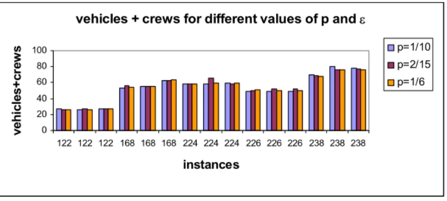
of p (1/10, 2/15, 1/6) were tested. Figure 1 shows the effect of the different

parameter values on the number of vehicles and crews in the final solution,

whereas Figure 2 shows the effect of the different parameter values on the CPU

times (in seconds).

Figure 1: Total number of vehicles+crews for different values of p and ε

vehicles + crews for different values of p and ε

0 20 40 60 80 100

122 122 122 168 168 168 224 224 224 226 226 226 238 238 238

instances

ve

hi

c

les

+

c

re

w

s p=1/10

p=2/15 p=1/6

Figure 2: Computing time for different values of p and ε

cpu for different values of p and ε

0 50 100 150 200 250 300 350

122 122 122 168 168 168 224 224 224 226 226 226 238 238 238

instances

cp

u

(

se

c) _p=1/10

p=2/15 p=1/6

Figure 1 shows that the quality of the VCP solutions did not change for the

different combinations of parameter values. However, Figure 2 reveals that a fine

tuning of the parameters can greatly reduce the CPU time.

The set of crew duties given by each final VCP solution is the input data for the

corresponding DRP instance. The DRP programs ran on a PC Pentium IV Dual

Core, 2 Duo 1.8 GHz. For each one of the resulting 45 DRP instances, three single

solved. In the first, λ₁=1 and λ₂ =0, that is, the DRP with the single objective

of minimizing the total number of drivers (minimize fr1 in (4.1)), whose

computational results are shown in Table 1. In the second, λ₁=0 and λ₂ =1 in

order to minimize the maximum overtime per driver during the rostering period

(minimize fr₂ in (4.1)) and the corresponding results are presented in Table 2.

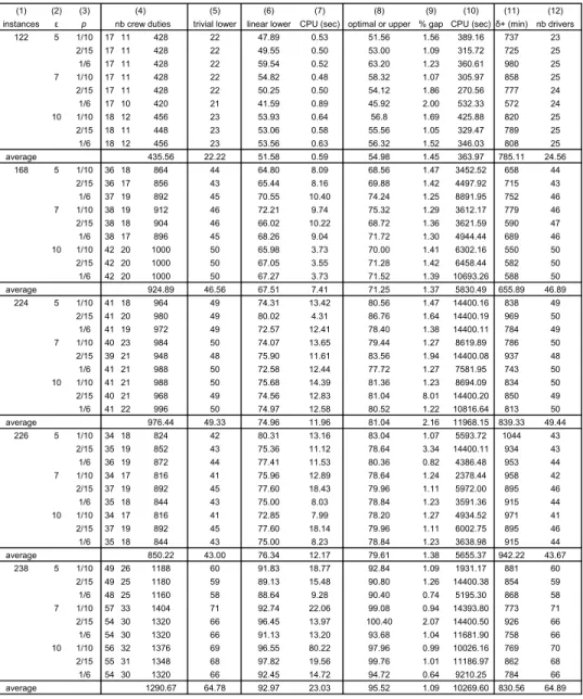
Finally, Table 3 presents results obtained with the third strategy, λ₁=0.96 _and

04 . 0

2 =

λ . These values balance the weighted value of both optimization

objectives for rostering, since the rate of the single objective values is about 1 to

24, for some representative instances.

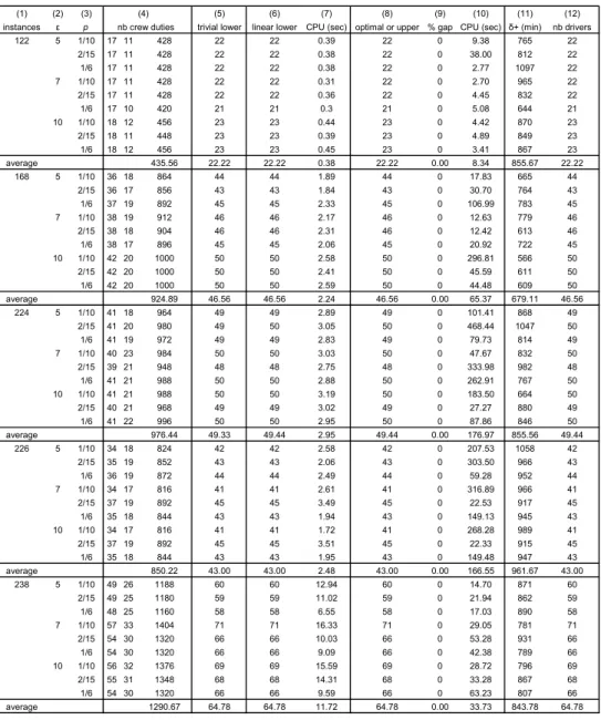
For the three tables, columns (1)-(5) retain the same meaning and values,

summarizing the features of the instances. Columns (1), (2) and (3) identify each

DRP instance depending on the VCRP problem data and on parameters of the

VCP solving process. Column (4) gives the number of crew duties per weekday

(from the solution of the VCP), the number of crew duties per weekend day

(determined on the assumption that in the area under study the timetables at

weekends cover neither early morning nor late evening trips) and the total number

of crew duties for the rostering period calculated by using the formula

6

1 ₂

5αL + αL , which has already been used in (4.4) for the general case.

Column (5) shows the value of the trivial lower bound for the minimum number

of drivers, calculated from (4.4).

In Tables 1 to 3, columns (6) and (7) present the optimal value of the MILP

formulation’s linear relaxation and the respective CPU time in seconds. Columns

(8) to (10) show, respectively, the MILP optimal value or the best upper bound

when the solver did not stop with the optimal solution (two stopping criteria were

established: a limit of four CPU hours and an “absolute mip” gap of 1 unit), the

relative gap in percentage (optimum or upper bound minus CPLEX last lower

bound divided by this lower bound, times 100) and the CPU time in seconds.

Column (11) displays the maximum overtime assigned to a driver during the

rostering period (in minutes) and column (12) the number of drivers assigned to

work during the rostering period. The values in both columns are calculated on the

basis of a specific roster as follows:

forcing fr1 to be equal to the minimum given in column (8) (in this table,

column (12) is equal to column (8));

– in Table 2, column (12), each value is obtained by minimizing fr1 subject to

(3.1)-(3.20), (3.24), (3.25), (4.2) and (4.3), as well as to an extra constraint

forcing fr2 to be less or equal to the minimum or upper bound given in

column (8) (in this table, column (11) is equal to column (8));

– in Table 3, columns (11) and (12) show the figures for fr2 and fr1 calculated

from a roster that corresponds to the weighted value in column (8).

Note that, considering the DRP as a bi-objective optimization problem, columns

(12) and (11) of the three tables indicate the coordinates of candidates to be

non-dominated points. In the case of Tables 1 and 2, these are the candidate

lexicographic points of the Pareto frontier. All these points are just candidates,

without the guarantee of being non-dominated points, because optimality stopping

condition was not attained when minimizing fr2.

(Insert Table 1 here)

(Insert Table 2 here)

(Insert Table 3 here)

The first observation that arises from the figures concerns the quality of the

trivial lower bound for the number of drivers assigned to work. As seen in

columns (5) and (8) of Table 1, the best value was found for all the 45 instances.

This happens with the current test problems, which is not only due to the low

dimension workforce required at weekends but also to the fact that the hard

constraints are not very restrictive, which in other real rostering situations may not

occur. However, the inclusion of this additional constraint improved the linear

lower bound and significantly reduced the computing time.

As, for the linear lower bounds (column 6), in Table 1, all except one are equal

to the corresponding optimal values (column 8). In the other cases, Tables 2 and

3, the linear lower bounds have a higher gap in relation to the best known upper

bound.

From these experiments one can observe that, for each instance, rosters

satisfying all the hard constraints (feasible rosters) were found in keeping with

different rostering strategies (from the three choices for λ₁ and λ₂), in reasonable

satisfaction of (soft1) and (soft2) can be seen in columns (12) and (11),

respectively.

The optimal solutions were easily found in short computing times in the case

of minimizing the number of drivers alone (see, Table 1, column (10)). But, when

optimizing the maximum overtime per driver, either alone (λ₁=0 and λ₂=1) or

combined with the workforce dimension (λ₁=0.96 and λ₂=0.04), the computing

efficiency was lower, as may be seen in Tables 2 and 3 (columns (8) and (10)).

The same happened also when minimizing fr2 subject to a fixed value for fr1, see

column (11) of Table 1. In fact, all these 45 MILP instances were not optimally

solved by the CPLEX algorithm due to excessive computing time (time limit of 4

CPU hours). Respecting the optimization of fr1 subject to an upper bound on the

value of fr2 (column (12) of Table 2) 17.8% instances were not solved within the

time limit and each one of the remaining was solved, on average, in 5741.8

seconds. It is also interesting to note that the computing time necessary to solve

the linear relaxation is not significantly higher for these difficult instances (see

columns (7) in Tables 2 and 3) than it is for the easy cases (column (7), Table 1).

To sum up, the results displayed on Tables 1 and 2 confirm the conflicting

nature of the two rostering objectives. As expected, the optimization of one

objective can only be obtained at the expense of the other. On the other hand,

Table 3 shows that it is possible to produce rosters that reconcile the interests of

both agents involved in the rostering process. However, in using the sequential

process for the VCRP, whether a single solution or a set of different solutions is

produced by the VCP algorithm, as in the experiment under study (nine VCP

solutions per VCRP problem), the objectives of rostering may not be satisfactorily

contemplated. In fact, as some statistical tests will show next, there is no

correlation between the quality of each VCP solution (fvc0) and the quality of the

corresponding DRP solution (

λ

₁fr₁+

λ

₂fr₂). Consequently, a complete

integration should be considered in the future.

For each of the 45 instances Figure 3 plots the vehicle and crew costs versus

the rostering costs whilst, for each test problem Table 4 presents the

corresponding correlation coefficient. The penalizing parameters λ₁and λ₂ for

the rostering problem, were set to λ₁=0.96 and λ₂=0.04.

35 45 55 65 75 85 95 105

150000 200000 250000 300000 350000 400000 450000 500000 550000

VCP costs

R

o

st

er

ing cost

s 122

168 224 226 238

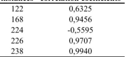
(Insert Table 4 here)

From Figure 3 and Table 4, one may conclude that there is no correlation

between the vehicle-crew costs and the rostering costs. In fact, excepting problem

238, the absolute values of the correlation coefficients range from 0.0263 to

0.2089.

Even when one considers just one of the objectives, there is no pattern for the

values of the correlation coefficients as shown on Tables 5 and 6.

(Insert Table 5 here)

(Insert Table 6 here)

In conclusion, given a new problem, one is unable to predict if “good”

solutions for the VCP will lead to good solutions for the DRP. The only way to

guarantee low vehicle costs and good rosters is to solve the integrated

vehicle-crew-roster problem.

6. Conclusions and Future Research

This paper presents an integrated formulation modeling public transit scheduling

problems. The vehicle schedule, the drivers’ schedule, as well as the rosters for

the drivers are obtained concurrently as opposed to being separately determined,

as is usually the case in other approaches.

It is well known that scheduling on public transit companies encompasses

can be hierarchically organized. The solution to each problem provides

information for the others. In fact, the vehicle schedule (definition of the vehicle

blocks) supports the definition of crew duties (work days) which, in turn, must be

assigned to drivers, over the rostering period, which leads to a roster. Due to their

individual complexity, the problems mentioned are usually handled separately and

in sequence, possibly leading to poor quality final solutions. As rostering relies on

the output of the other two schedules, one cannot guarantee that the final result is

the best solution to the overall problem.

Typically, rostering applies to a period including several VCP planning

periods (or days) and, due to its larger extent, it must combine sequencing

constraints with a broader spectrum. Furthermore, an attempt to anticipate some

of these constraints, while solving the VCP, may lead to non-optimal global

solutions. For instance, take the case of a set of crew duties coming from the VCP,

some very long, others very short, each one to be assigned to a single driver

during a day. Perhaps, if timetabled trips and/or tasks were combined in another

way, eventually leading to worse results for vehicle and crew optimization, from

the rostering and even from the global VCRP standpoint, they would produce

better solutions. In fact, crew duties arrive at the rostering phase as data, with no

possibility of adjustments.

Previous experience has revealed that an integrated approach for the vehicle

and crew scheduling problems is accomplishable and provides high quality

solutions, Mesquita and Paias (2008) and Mesquita et al. (2006) thus pointing to

an extension to accommodate rostering decisions as well. As a result, this paper

proposes a multi-objective mixed binary linear programming formulation for the

integrated vehicle-crew-rostering problem, modeling the different decisions and

constraints arising in the operational planning phase in public transit companies.

This monolithic model is approached by solving the integrated vehicle and crew

scheduling problem for different values of the VCP parameters, hence producing a

diverse set of final solutions. Afterwards, the resulting rostering problems are

solved. One such approach may be the basis of a decision support system able to

indicate to the user the effects of parameters in the final solutions and, at the same

time, to produce a diversity of vehicle schedules and rosters.

Moreover, it should be emphasized that the driver rostering problem analyzed

deals with a planning situation where rest periods are imposed, where different

durations for the rostering period may be considered, where one must take into

account the tasks performed by the drivers beforehand, in the last days of the

previous period, when one allows for different demand patterns of transport from

day to day, and where a multitude of other scheduling rules can be introduced.

Within this process, the rostering is naturally guided by two optimization

objectives: minimization of driver costs and balancing of overtime work,

representing the interests of the management and of the drivers of the company

respectively. Note that not only public transit companies but also other transport

companies share similar requirements as regards the rostering process.

Acknowledgements

The authors would like to thank to Dulce Pedrosa and Rita Portugal for all the explanations and

the data they made available to us. The research was funded by POCTI/ISFL/152and

PPCDT/MAT/57893/2004.

References

Aringhieri, R., Cordone, R. (2004). The Multicommodity Multilevel Bottleneck Assignment

Problem. Electronic Notes in Discrete Mathematics, 17, 35-40.

Ball, M.O., Bodin, L.D., & Dial, R. (1983). A Matching Based Heuristic for Scheduling Mass

Transit Crews and Vehicles. Transportation Science, 17, 4-31.

Barnhart, C., & Laporte, G. (eds.) (2007). Transportation. Handbooks in Operations Research and

Management Science, 14. Elsevier, North-Holland, Amsterdam, Holland.

Borndröfer, R., Grötchel, M., Pfetsch, M. (2006). Can O.R. Methods Help Public Transportation

Systems Break Even? German Research Group Moves Industry Close to Elusive Goal. OR/MS

Today, 33, 30-40.

Borndörfer, R., Löbel, A., & Weider, S. (2004). A Bundle Method for Integrated Multi-Depot

Vehicle and Duty Scheduling Public Transit. ZIB-Report 04-14. Zuse Institute Berlin, Germany.

Cappanera, P., & Gallo, G. (2004). A Multicommodity Flow Approach to the Crew Rostering

Problem. Operations Research, 52, 583-596.

Caprara, A., Monacci, M., & Toth, P. (2001). A Global Method for Crew Planning in Railway

Applications. In Voss S., Daduna J. (eds.), Computer-Aided Scheduling of Public Transport.

Lecture Notes in Economics and Mathematical Systems, 505. Springer, Berlin, Germany, 17-36.

Caprara, A., Toth, P., Vigo D., & Fischetti, M. (1998). Modeling and Solving the Crew Rostering

Problem. Operations Research, 46, 820-830.

Carraresi, P., & Gallo, G. (1984). A Multi-level Bottleneck Assignment Approach to the Bus

Catanas, F., & Paixão, J.M.P., (1995). A New Approach for the Crew Rostering Problem. In

Daduna, J., Branco, I.M., Paixão J.M.P. (eds.), Computer-Aided Scheduling of Public Transport.

Lecture Notes in Economics and Mathematical Systems, 430. Springer, Berlin, Germany, 267-277.

CPLEX Manual (version 9.0) (2003) Using the CPLEXR Callable Library and CPLEX Mixed

Integer Library. ILOG INC., Incline Village, Nevada, USA.

CPLEX Manual (version 11). (2007). Using the CPLEXR Callable Library and CPLEX Mixed

Integer Library. ILOG INC., Incline Village, Nevada, USA.

Chu, S.C.K. (2007). Generating, Scheduling and Rostering of Shift Crew-Duties: Applications at

the Hong Kong International Airport. European Journal of Operational Research, 177, 1764-1778.

Dantzig, G. (1954). A Comment on Edie’s Traffic Delay at Toll Booths. Operations Research, 2,

339-341.

De Groot, S., & Huisman, D. (2004). Vehicle and Crew Scheduling: Solving Large Real-World

Instances with an Integrated Approach. Econometric Institute Report EI2004-13, Erasmus

University, Rotterdam, The Netherlands.

Ernst, A., Jiang, H., Krishnamoorthy, M., Nott, H., & Sier, D. (2001). An Integrated Optimization

Model for Train Crew Management. Annals of Operations Research, 108, 211-224.

Ernst, A., Jiang, H., Krishnamoorthy, M., & Sier, D. (2004). Staff Scheduling and Rostering: A

Review of Applications, Methods and Models. European Journal of Operational Research, 153,

3-27.

Freling, R., Huisman, D., & Wagelmans, A.P.M., (2003). Models and Algorithms for Integration

of Vehicle and Crew Scheduling. Journal of Scheduling, 6, 63-85.

Freling, R., Lentink, R.M., & Wagelmans, A.P.M., (2004). A Decision Support System for Crew

Planning in Passenger Transportation Using a Flexible Branch-and Price Algorithm. Annals of

Operations Research, 127, 203-222.

Freling, R., Wagelmans, A.P.M., & Paixão, J.M.P. (1999). An Overview of Models and

Techniques for Integrating Vehicle and Crew Scheduling. In Wilson, N.H.M. (ed.),

Computer-Aided Transit Scheduling. Lecture Notes in Economics and Mathematical Systems 471. Springer,

Berlin, Germany, 441-460.

Haase, K., Desaulniers, G., & Desrosiers, J. (2001). Simultaneous Vehicle and Crew Scheduling in

Urban Mass Transit Systems. Transportation Science, 35(3), 286-303.

Haase, K., & Friberg, C. (1999). An Exact Branch and Cut Algorithm for the Vehicle and Crew

Scheduling. In Wilson N.H.M. (ed.), Computer-Aided Transit Scheduling. Lecture Notes in

Economics and Mathematical Systems, 471. Springer, Berlin, Germany, 63-80.

Hartog, A., Huisman, D., Abbink, E.J.W., & Kroon, L.G. (2006). Decision Support for Crew

Rostering at NS. Econometric Institute Report EI2006-04, Erasmus University, Rotterdam, The

Netherlands.

Hollis, B.L., Forbes, M.A., & Douglas, B.E. (2006). Vehicle Routing and Crew Scheduling for

Metropolitan Mail Distribution at Australia Post. European Journal of Operational Research, 173,

133-150.

Huisman, D., Freling, R., & Wagelmans, A.P.M. (2005). Multiple-Depot Integrated Vehicle and

Kohl, N., & Karisch, S.E. (2004). Airline Crew Rostering: Problem Types, Modeling, and

Optimization. Annals of Operations Research, 127, 223-257.

Lee, C.-K., & Chen, C.-H. (2003). Scheduling of Train Drivers for Taiwan Railway

Administration. Journal of Eastern Asia Society of Transportation Studies, 5, 292-306.

Lezaun, M., Pérez, G., & Maza, E.S. (2006). Crew Rostering Problem in a Public Transport

Company. Journal of the Operational Research Society, 57, 1173-1179.

Lucic, P., & Teodorovic, D. (1999). Simulated Annealing for the Multi-objective Aircrew

Rostering Problem. Transportation Research Part A, 33, 19-45.

Lucic, P., & Teodorovic, D. (2007). Metaheuristics approach to the aircrew rostering problem.

Annals of Operations Research, 155, 311-338.

Mesquita, M., Paias, A., & Respício, A. (2006). Branching approaches for the integrated vehicle

and crew scheduling problem. Working paper 9/2006, Centro de Investigação Operacional,

Faculdade de Ciências da Universidade de Lisboa, Portugal. (available at

http://cio.fc.ul.pt/home.do).

Mesquita, M., & Paias, A. (2008). Set partitioning/covering-based approaches for the integrated

vehicle and crew scheduling problem. Computers and Operations Research, 35 (5) , 1562-1575.

Mesquita, M., & Paixão, J.M.P., (1992). Multiple Depot Vehicle Scheduling Problem: A New

Heuristic Based on Quasi-Assignment Algorithms. In Desrochers, M., Rousseau, J.M. (eds.),

Computer-Aided Transit Scheduling. Lecture Notes in Economics and Mathematical Systems,

386. Springer, Berlin, Germany, 167-180.

Moz, M., & Pato, M.V. (2007). A Genetic Algorithm Approach to a Nurse Rerostering Problem.

Computers and Operations Research, 34, 667-691.

Moz, M., Respício, A., & Pato, M.V. (2007). Bi-objective Evolutionary Heuristics for Bus Drivers

Rostering. Working paper 1/2007, Centro de Investigação Operacional, Faculdade de Ciências da

Universidade de Lisboa, Portugal. (available at http://cio.fc.ul.pt/home.do).

Figure legends

Figure 1: Total number of vehicles+crews for different values of p and ε

Figure 2: Computing time for different values of p and ε

Tables

Table 1: Computational results from DRP problems withλ1=1 and λ2 =0

(1) (2) (3) (4) (5) (6) (7) (8) (9) (10) (11) (12)

instances ε p nb crew duties trivial lower linear lower CPU (sec) optimal or upper % gap CPU (sec) δ+ (min) nb drivers

122 5 1/10 17 11 428 22 22 0.39 22 0 9.38 765 22

2/15 17 11 428 22 22 0.38 22 0 38.00 812 22

1/6 17 11 428 22 22 0.38 22 0 2.77 1097 22

7 1/10 17 11 428 22 22 0.31 22 0 2.70 965 22

2/15 17 11 428 22 22 0.36 22 0 4.45 832 22

1/6 17 10 420 21 21 0.3 21 0 5.08 644 21

10 1/10 18 12 456 23 23 0.44 23 0 4.42 870 23

2/15 18 11 448 23 23 0.39 23 0 4.89 849 23

1/6 18 12 456 23 23 0.45 23 0 3.41 867 23

average 435.56 22.22 22.22 0.38 22.22 0.00 8.34 855.67 22.22

168 5 1/10 36 18 864 44 44 1.89 44 0 17.83 665 44

2/15 36 17 856 43 43 1.84 43 0 30.70 764 43

1/6 37 19 892 45 45 2.33 45 0 106.99 783 45

7 1/10 38 19 912 46 46 2.17 46 0 12.63 779 46

2/15 38 18 904 46 46 2.31 46 0 12.42 613 46

1/6 38 17 896 45 45 2.06 45 0 20.92 722 45

10 1/10 42 20 1000 50 50 2.58 50 0 296.81 566 50

2/15 42 20 1000 50 50 2.41 50 0 45.59 611 50

1/6 42 20 1000 50 50 2.59 50 0 44.48 609 50

average 924.89 46.56 46.56 2.24 46.56 0.00 65.37 679.11 46.56

224 5 1/10 41 18 964 49 49 2.89 49 0 101.41 868 49

2/15 41 20 980 49 50 3.05 50 0 468.44 1047 50

1/6 41 19 972 49 49 2.83 49 0 79.73 814 49

7 1/10 40 23 984 50 50 3.03 50 0 47.67 832 50

2/15 39 21 948 48 48 2.75 48 0 333.98 982 48

1/6 41 21 988 50 50 2.88 50 0 262.91 767 50

10 1/10 41 21 988 50 50 3.19 50 0 183.50 664 50

2/15 40 21 968 49 49 3.02 49 0 27.27 880 49

1/6 41 22 996 50 50 2.95 50 0 87.86 846 50

average 976.44 49.33 49.44 2.95 49.44 0.00 176.97 855.56 49.44

226 5 1/10 34 18 824 42 42 2.58 42 0 207.53 1058 42

2/15 35 19 852 43 43 2.06 43 0 303.50 966 43

1/6 36 19 872 44 44 2.49 44 0 59.28 952 44

7 1/10 34 17 816 41 41 2.61 41 0 316.89 966 41

2/15 37 19 892 45 45 3.49 45 0 22.53 917 45

1/6 35 18 844 43 43 1.94 43 0 149.13 945 43

10 1/10 34 17 816 41 41 1.72 41 0 268.28 989 41

2/15 37 19 892 45 45 3.51 45 0 22.33 915 45

1/6 35 18 844 43 43 1.95 43 0 149.48 947 43

average 850.22 43.00 43.00 2.48 43.00 0.00 166.55 961.67 43.00

238 5 1/10 49 26 1188 60 60 12.94 60 0 14.70 871 60

2/15 49 25 1180 59 59 11.02 59 0 21.94 862 59

1/6 48 25 1160 58 58 6.55 58 0 17.03 890 58

7 1/10 57 33 1404 71 71 16.33 71 0 29.05 781 71

2/15 54 30 1320 66 66 10.03 66 0 53.28 931 66

1/6 54 30 1320 66 66 9.09 66 0 42.38 789 66

10 1/10 56 32 1376 69 69 15.59 69 0 28.72 796 69

2/15 55 31 1348 68 68 14.31 68 0 33.28 867 68

1/6 54 30 1320 66 66 9.59 66 0 63.23 807 66