Ciências Sociais e Humanas
On the Relationship between Religiosity, Human Capital
and Income
Ricardo Manuel Neves Viegas
Dissertação para obtenção do Grau de Mestre em
Economia
(2
ociclo de estudos)
Orientador: Prof. Doutor Tiago Miguel Guterres Neves Sequeira
Agradecimentos
A realização desta dissertação marca o fim de uma importante etapa da minha vida. Gostaria de agradecer a todos aqueles que contribuíram de forma decisiva para a sua concretização.
À Universidade da Beira Interior pela possibilidade de realização do presente trabalho, por todos os meios colocados à disposição e pela excelência da formação prestada e conhecimentos transmitidos, que foram úteis para a elaboração desta dissertação, ambicionando que esta dignifique a instituição. Ao meu orientador deste trabalho Professor Doutor Tiago Sequeira pela disponibilidade, colabo-ração, transmissão de conhecimentos e capacidade de estímulo, bem como pela amizade e estima pessoal demonstrada.
À minha família um profundo e sentido reconhecimento pelo apoio incondicional ao longo destes anos.
Aos meus amigos de longa data e colegas da UBI agradeço a força, a amizade e a confiança que depositaram em mim.
A todos que me ajudaram a ser quem sou, que depositaram confiança em mim e para comigo têm altas expectativas, resta-me afincadamente não vos desiludir. Bem hajam...
Resumo
A literatura empírica recente tem abordado a relação entre o rendimento e a religião. Maioritaria-mente, esta ligação baseia-se no efeito positivo que as crenças religiosas têm no trabalho produtivo (argumento Weberiano) ou no efeito negativo que a adesão a serviços de carácter religioso tem na diminuição das horas de trabalho. Assim, o capital humano é o fator de produção que é potenci-almente mais afetado pela religião. Apesar disso, a relação entre o capital humano e a religião a nível agregado não tem tido a enfase adequada. Assim, apresento uma nova influência não-linear da participação religiosa das crianças na formação do capital humano. Esta relação é robusta no que toca à heterogeneidade e estacionaridade das variáveis entre países, bem como na existência de crenças não-observáveis. Quando a causalidade é tida em conta, o efeito positivo e robusto da religião no capital humano mantém-se, em oposição aos resultados mais recentes, que tendem para um efeito negativo. A maioria dos estudos é baseada em micro-dados, e macro-dados que ignoram largamente a potencial heterogeneidade entre países. Usando dados retrospetivos de taxas de participação religiosa para um painel de países entre 1925 e 1990, aplico estimadores de hetero-geneidade em painel e revelo que o efeito da participação em atividades religiosas no rendimento per capita é maioritariamente não significante. Isto é consistente com algumas pesquisas recentes que suscitam dúvidas sobre a influência da religião no rendimento, quando a causalidade é tida em conta.
Palavras-chave
Resumo Alargado
A literatura empírica recente tem abordado a relação entre o rendimento e a religião. Maioritaria-mente, esta ligação baseia-se no efeito positivo que as crenças religiosas têm no trabalho produtivo (argumento Weberiano) ou no efeito negativo que a adesão a serviços de carácter religioso tem na diminuição das horas de trabalho. Assim, o capital humano é o fator de produção que é potenci-almente mais afetado pela religião. Apesar disso, a relação entre o capital humano e a religião a nível agregado não tem tido a enfase adequada. Assim, apresento uma nova influência não-linear da participação religiosa de crianças na formação do capital humano. Esta relação é robusta no que toca à heterogeneidade e estacionaridade das variáveis entre países, bem como na existência de crenças não-observáveis. Quando a causalidade é tida em conta, o efeito robusto positivo da religião no capital humano mantém-se, em oposição aos resultados mais recentes, que apresentam um efeito negativo. A maioria dos estudos é baseada em micro-dados, e maco-dados que ignoram largamente a potencial heterogeneidade entre países. Usando dados retrospetivos de taxas de parti-cipação religiosa para um painel de países entre 1925 e 1990, aplico estimadores de heterogeneidade em painel e revelo que o efeito da participação em atividades religiosas no rendimento per capita é maioritariamente não significante. Isto é consistente com algumas pesquisas recentes que suscitam dúvidas sobre a influência da religião no rendimento, quando a causalidade é tida em conta. Neste trabalho, depois dos índices, é apresentada uma introdução a este tema complementada com uma revisão da literatura já existente. De seguida são apresentados dois capítulos, referindo-se o primeiro à relação entre a religião e o capital humano e o segundo à relação entre a religião e o crescimento económico. O primeiro capítulo é constituído por três subcapítulos onde são denotados, por esta ordem, os dados usados e as respetivas fontes, os métodos e estimativas postas em prática, e os resultados obtidos. Dentro deste último subcapítulo é ainda dada uma achega aos efeitos de causalidade existentes. O segundo capítulo é repartido em dois subcapítulos, sendo no primeiro apresentada a revisão da literatura referente à relação entre a religião e o rendimento. No segundo é explicada a relação teórica entre ambos e apresentados os dados usados e respetivas fontes, bem como as estimativas e métodos postos em prática. Ainda neste subcapítulo são apresentados os resultados obtidos, fazendo referência à robustez do modelo apresentado. Para terminar são apresentadas as conclusões obtidas com este estudo.
Abstract
A recent empirical literature has addressed the relationship between income and religion. The argument that links religion to income is mainly based on the positive effect religious beliefs has on labor productivity (Weberian argument) or on the negative effect that attending religious services has on decreasing labour supply. Thus human capital is the production factor which is potentially most affected by religion. Despite of that, the relationship between human capital and religion at the aggregate level has been overlooked. I present a new nonlinear influence of religious attendance by children in the formation of human capital. This relationship is robust to country heterogeneity and variable stationarity and to the existence of nonobservable beliefs. Once reverse causality is taken into account, a robust positive effect of religion on human capital subsists, in opposition to the most recent results, which seem to point to a negative effect. Most studies are based on microdata, and macroeconomic analysis of the issue that has largely ignored the potential heterogeneity between countries. Using retrospective data on church attendance rates for a panel of countries between 1925 and 1990, I apply heterogeneous panel data estimators and reveal that the effect of participation in religious activities on income per capita is mostly non-significant. This is consistent with some of the recent research that casts doubt onto the influence of religion on income, once causality is taken into account.
Keywords
Índice
1 Introduction 1
2 Human Capital and Religion: A new nonlinear relationship 4
2.1 Data and Sources . . . 4
2.2 Estimation and Methods . . . 5
2.3 Results . . . 7
2.3.1 Further addressing causality . . . 8
3 Income and Religion: A heterogeneous panel data analysis 10 3.1 The effect of Religion on Income . . . 10
3.2 Empirical Relationship between Religion and Income . . . 13
3.2.1 Data and Sources . . . 13
3.2.2 Estimation and Methods . . . 14
3.2.3 Results . . . 17
3.2.4 Robustness . . . 18
4 Conclusion 20 5 Bibliography 22 A Attachments 26 A.1 Religious Attendance and the investment share . . . 26
A.2 Countries in regressions 2-4 Table 2.3 (25) . . . 26
A.3 Countries in regression 3, Table 2.3 (24) . . . 27
A.4 Countries in regressions 1-3 of Table 2.4 (22) . . . 27
A.5 Countries in regression 4 of Table 2.4 (21) . . . 27
Lista de Figuras
2.1 Religion (children) Attendance by Country, 1925-1990 . . . 6
3.1 Theoretical Relationship between Religion and Income . . . 12
3.2 Religion (children) Attendance by Country, 1925-1990 . . . 15
Lista de Tabelas
2.1 Descriptive Statistics . . . 5
2.2 Cross-sectional dependence and Unit Root tests . . . 6
2.3 Human Capital and Religion in Heterogeneous Panels . . . 8
2.4 Human Capital and Religion in Heterogeneous Panels with weak exogenous Religion 9 3.1 Descriptive Statistics . . . 14
3.2 Cross-Sectional Dependence and Unit Root Tests . . . 16
3.3 Income and Religion in Heterogeneous Panels . . . 19
Capítulo 1
Introduction
Since the beginning of humanity, men kind has a mysterious fascination for mythology. With his evolution, the beliefs on the unknown forces and supernatural events has evolved in many religions. Influenced by the environment, culture and geographic location, many different religions have been created in order to give men kind a sense in their lives. Religion is in every action, in every day. It influences who we are, who we want to be and the relations we have with others, but also affects our personal economy.
So, one can think that religion has a mutual effect with income and economic growth. This was what Weber (1930) thought. Theoretically, there are several potential positive and negative effects of religion in the wealth of individuals and countries, as mostly people can’t leave without religion. This is due to the simple fact that man finds in religion some of his meaning of live, or because his parents were religious and he has a religious education that made him a religious one, or because he hopes that there is a life after death and pray to reach the life he beliefs.
Religion attendance take some time to accomplish and as the most scarce resource, time is needed to work, produce, sell and buy. But also is true that religions and their events promotes local economy by their own means. And, religious values may include work ethic, honesty (and hence trust), thrift, charity, hospitality to strangers and so on (McCleary and Barro, 2006), some of which might be drivers of income. For instance, Andersen et al (2012) showed that cultural values influenced by the Cistercians’ Catholic order may explain differential development in English countries.
In other contexts, the powerful force from afterlife beliefs can promote anti-social actions, such as violence - the so-called dark side of religion (McCleary and Barro, 2006). Additionally, there is some trade-off between participation in religious activities and income-led activities and religion may also decrease the utility driven by consumption (see e.g. Bettendorf and Dijkgraaf, 2011). But if religion can effect growth, income may also affect religion through secularization - an effect of increases in education and scientific knowledge, as thus the issue of causality between income and religion arises (see McCleary and Barro, 2006).
So, as easily any one can observe, human capital is the most directly production factor affected by religion. The empirical results obtained so far are quite controversial and a consensus on the casual effect of religion on growth and income is far from been achieved.
In this theme, the main bulk of the literature consists of analysing the effects of religion mem-bership on labour earnings (Chiswick, 1983; Tomes, 1984; Tomes, 1985; Chiswick, 1993; Sten, 1996; Cornwell et al, 2003; Bettendorf and Dijkgraaf, 2011; Cornelissen and Jirjahn, 2012). These papers are single country micro-data studies covering mainly the US and Canada. When looked as a whole, the obtained results are not conclusive. In most of them the statistical significance depends on the religion considered or on the measure (membership or participation). When taking into account a bicausal relationship between religion and income, Bettendorf and Dijkgraaf (2011) found a nonsignificant relationship. Thus they conclude that possible statistical significance was obtained due to the ignorance of the causality nexus. Some more recent papers have analysed the effect of religion on individual attitudes which are "good"for growth and conclude that in general religious beliefs or membership are associated with good economic attitudes (Guiso et al, 2003 and Renneboog and Spaenjers, 2012).
A smaller set of the literature tried to estimate cross-country or cross-regional effects of religion on income. Heath et al. (1995) study the issue using a cross-section of US states and found different effects on per capita income depending on the religion. Lipford and Tollison (2003) also uses religious membership to explain different income per capita in US states (with a different model than Heath et al. (1995) and not distinguish between religious) but found a robust negative effect. Crain and Lee (1999) implement growth regression to US states and conclude for a nonsignificant effect of religious membership on growth. Barro and McCleary (2003) study a cross-section of 58 countries and they concluded that membership and participation have a negative effect on economic growth but beliefs have a positive effect. The first article that explores the time-series dimension of the relationship between religion and income, also accounting for heterogeneity between countries, was Mangeloja (2005). From the eight countries studied, there is only one country with a positive effect of religious efficiency (belief * participation), two countries with negative effects and one with positive effect of participation. This has called the researchers attention to the great heterogeneity between countries in what the relationship between religion and income is concerned, an issue also confirmed by Bettendorf and Dijkgraaf (2011) in a sample of 25 western countries. Dierk and Strulik (2013) found a negative long-run cointegrated relationship between religion and income per capita in 17 (developed) countries, using panel data methods that explore the time-series dimension but do not fully accounts for heterogeneous slopes between countries.
Historical evidence is also quite contradictory concerning the effects of religion on income. Becker and Woessmann (2009) showed a significant negative effect of religion on literacy, using IV and OLS estimates for Prussian countries in the 19th century. However, the same authors (Becker and Woessmann, 2013) showed that the influence of religion on income per capita in Prussian countries turns out to be nonsignificant in panel analysis. Blum and Dudley (2001) found that wages grew more in protestant pre-industrial (1500-1750) European cities than in its catholic counterparts. However, Cantoni (2013), using data for German cities between 1300 and 1900, found no effects of Protestantism on economic growth.
A first insight from the comparison of micro and macro studies is that while the first concentrates on the effect on labour productivity or earnings, close to the definition of human capital, the second concentrates in the analysis of the effect on income. Exceptions are Becker and Woessmann (2009), which analysed the effect of religion in Prussian countries literacy and Berggren and Bjornskov (2013) which analysed links between religion and property rights. Overall the relationship or influence of religion in human capital is overlooked in the macro-level literature. With this study this gap is intended to fill. In fact, there are strong reasons to believe that the main channel through which religion may affect income and growth is human capital. First, almost all the micro literature has shown relationship between religion and labor earnings, which is a variable linked to human capital and its returns. Second a couple of references had shown evidence of a relationship between human capital and religion. One is Becker and Woessmann (2009) finding a positive effect of religion on Prussia’s counties literacy in the nineteenth century. Another is Meredith (2011) who found that enrollment growth in religiously affiliated institutions is higher than in private secular institutions. Third, the earlier arguments that initiated the quest for an influence of religion on income are linked with human capital. As is evident from the analysis on McCleary and Barro (2006), religious beliefs may enhance human attributes which in turn enhance productivity (in learning or workplace). As an opposite effect, beliefs can also act as a substitute for learning (scientific knowledge).
So, since the beginning of this discussion (Weber, 1930), most of the investigation has addressed the microeconomic empirical relationship between religion and labour earnings. The macro lite-rature has concentrated on the empirical relationship between religion and economic growth and
differences in income between countries, thus concentrating on the long-run relationship between religion and income. Both the macro and the microeconomic literature have achieved contradictory results concerning the sign of the effect of religion on wages, economic growth, and income diffe-rences. This happens despite the fact that some authors consider that some religion-driven values are important for growth of countries. On the other hand, some of the most recent macroeconomic findings point out to a non-significant effect of religion on growth.
The literature has incorporated issues such as reverse causality and other forms of endogeneity, but mostly ignored heterogeneity between countries, common factors affecting the relationship between religion and income, and distinctions between the short and long run. In this study, I pretend to incorporate those factors in a panel estimation. This study incorporates these factors in a panel data estimation.
Capítulo 2
Human Capital and Religion: A new nonlinear relationship
2.1 Data and Sources
Until now, the data on religious attendance are mostly based on specific data surveys for one or various countries. This implies that a complete panel data for religious attendance was unavailable until Iannaccone (2003), who provided a dataset on religious attendance in 32 countries from 1925 to 1990.1 The idea of Iannaccone’s study was to estimate historical church attendance rates using
contemporary International Social Survey Programme (ISSP) questionnaires and replies to inquires on church attendance when the respondents were 11 or 12 years old. Naturally, this retrospective method could be harmed by different sorts of biases (e.g. age effects or projection bias). Iannac-cone therefore presents strong arguments that demonstrate that there is no reason for concern. I base on the literature on determinants of education to select the main macroeconomic determi-nants that have been shown to have robust effects on education. Hanushek and Woessmann (2011) argue that variations in skills measured by the international tests are in turn strongly related to individual labor-market outcomes and, perhaps more importantly, to cross-country variations in economic growth. There is also strong empirical evidence for the effect of parental income in scho-oling outcomes. According to this evidence I will use an expenditure measure of GDP to account for this income effect on skills. Additionally, Hazan (2012) and Oster et. al. (2013) show evidence for a positive effect of life expectancy at birth on education. I also use life expectancy at birth as a determinant of human capital. There are other possible determinants of education which have been explored in the literature. However, evidence for the robustness of those determinants are less strong than for income and life expectancy. I will also consider two additional variables: Assassi-nations and the Openness ratio in specific robustness specifications, which is explained in the next section. Although Innacone (2003) provided data for religious attendance of adults and children, in this section I use religious attendance of children as this is more related to the accumulation of human capital that I used, which is totally related to education and with a special weight to primary education.2 For variables other than religion attendance I use the Penn World Tables 8.0
(Feenstra et. al., 2013), the World Bank and Databanks International. Human capital index is from PWT 8.0 (Index of human capital per person, based on years of schooling from the Barro and Lee database (Barro and Lee, 2013) and returns to education (Psacharopoulos, 1994)), income is the expenditure-side real GDP per capita at chained PPPs (US $) from PWT 8.0. Openess ratio is the ratio of exports plus imports on GDP, also from PWT 8.0. Life expectancy is from the World
1The countries in Innaccone database are: Australia, Austria, Bulgaria, Canada, Chile, Cyprus, Czech
Republic, Denmark, France, West Gernamy, East Germany, Great Britain, Hungary, Ireland, Italy, Ja-pan, Latvia, Netherlandas, New Zealand, Northern Ireland, Norway, Phillipines, Poland, Portugal, Russia, Slovakia, Slovenia, Spain, Sweden, Switzerland and United States. I disregard Northern Ireland in the em-pirical exercise and constructed a population-weighted average of the measures of West and East Germany to match Germany in the empirical exercise. Although originally this source supplies data in a five-year interval, I have linearly extrapolated within the five-year interval to obtain yearly observations between 1925 and 1990. This procedure was also used by the PWT 8.0 to construct the human capital variable.
2To see why the PWT 8.0 measure of human capital is mainly weighted by primary education please
Bank. Finally, Assassinations come from the Databanks International. Descriptive statistics are presented in Table 2.1.
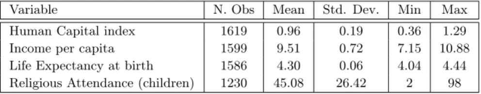
Tabela 2.1: Descriptive Statistics
Variable N. Obs Mean Std. Dev. Min Max
Human Capital index 1619 0.96 0.19 0.36 1.29
Income per capita 1599 9.51 0.72 7.15 10.88
Life Expectancy at birth 1586 4.30 0.06 4.04 4.44
Religious Attendance (children) 1230 45.08 26.42 2 98
Notes: Human capital, Income per capita, and life expectancy are in natural logarithms.
2.2 Estimation and Methods
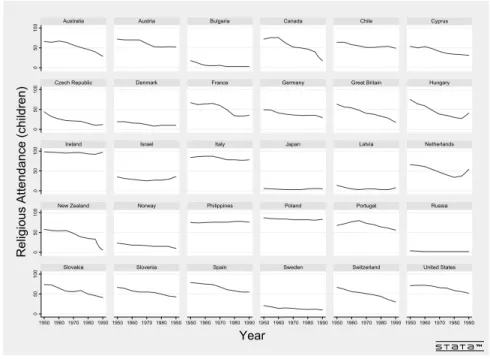
Heterogeneity and cross-section dependence in macro data has been extensively documented (see a survey in Eberhardt and Teal, 2011 and a empirical applications in Eberhardt and Teal, 2013a, 2013b and Eberhardt and Presbitero, 2014). I document here heterogeneity in religion attendance. Figure 2.1 is clear about different patterns of religious attendance across countries and also seems to indicate nonstationarity of these variables, which was also documented in Dierk and Strulik (2013). Table 2.2 presents results of the cross-sectional dependence test of Pesaran (2004) and of the Pesaran (2007) unit-root test which clearly reject the null for no cross-section dependence and do not reject the null for a unit-root for some of the regressors (life expectancy and religious attendance), invalidating traditional approaches for panel data econometrics.3 Thus I will use
the Pesaran (2006) common correlated effects mean group estimator to address my empirical objective. One of the important features of this estimator in comparison to other panel data estimators is that it is robust both to country-fixed effects such as geography, culture or initial religion-related beliefs and to unobservable common variables such as common productivity change (TFP) or common evolution of religious thinking or events to which beliefs within countries may react differently.4 Additionally, the method is robust to a type of endogeneity in which common
factors can simultaneously affect income or any of the regressors. Thus, if I consider common factors within religions that are linked with the evolution of beliefs, they can simultaneously affect income and religious attendance, which seem to be very reasonable to assume. Moreover, this estimator is also robust to the presence of stationary and non-stationary regressors.
The basic equation of interest in my analysis of the religion-income relationship is the following neoclassical production function augmented with religious attendance:
hit= β1iyit+ β2ileit+ β3iRit+ β4iR2it+ uit; uit= αi+ λ0ift+ εit, (2.1)
where h is the natural logarithm of human capital, y is the natural logarithm of per capita GDP, le is the log of the life expectancy at birth, R is religious (children) attendance as defined above, ft
is the vector of unobservable common factors and λ0
i is the associated vector of factor loadings, αi
3One should notice that the fact that human capital and also income reject the stationarity hypothesis
is due to the fact that I am working with a sample of relatively developed countries.
4This is consistent with initial country specific beliefs that evolve differently in each country due to
common factors which affects religions as a whole (e.g. the Second Vatican council; the election of new popes; the increase in new cults or sects) or other common factors such as the technological evolution.
Figura 2.1: Religion (children) Attendance by Country, 1925-1990 0 50 10 0 0 50 10 0 0 50 10 0 0 50 10 0 0 50 10 0 1950 1960 1970 1980 1990 1950 1960 1970 1980 1990 1950 1960 1970 1980 1990 1950 1960 1970 1980 1990 1950 1960 1970 1980 1990 1950 1960 1970 1980 1990
Australia Austria Bulgaria Canada Chile Cyprus
Czech Republic Denmark France Germany Great Britain Hungary
Ireland Israel Italy Japan Latvia Netherlands
New Zealand Norway Philippines Poland Portugal Russia
Slovakia Slovenia Spain Sweden Switzerland United States
Re lig io us A tte nd an ce (c hi ld re n) Year
Tabela 2.2: Cross-sectional dependence and Unit Root tests
(1) (2) (3) (4)
Variable Human Capital Income per
capita Life expectancy (at birth) Religious Attendance (children) CD T est 132.36*** 121.91*** 126.85*** 81.96*** (p-value) (0.000) (0.000) (0.000) (0.000)
Unit Root Test -5.510*** -1.314* 0.014 0.625
(p-value) (0.000) (0.094) (0.505) (0.734)
Note: Level of significance: *** for p-value<0.01; **for p-value<0.05;* for p-value<0.1. Human capital, Income per capita, and life expectancy are in natural logarithms. The cross-sectional dependence test is the Pesaran (2004) test under the null of no cross-section
dependence. The unit root test is the Pesaran (2007) test with one lag and no trend which tests the null of I(1) series.
are country-fixed effects and εitis the error term. As can be observed from (2.1), each coefficient is
country-specific, thus allowing for complete heterogeneity in the estimation. Additionally, as each regressor can also depend on the common factor, the method is also robust to endogeneity of the observable factors toward the common factors determining income. Rmax
it = 2ββ3i4i (where βi is the
averaged coefficient) is the level of religion that guarantees the maximum human capital level, i.e. this is the threshold level of religious attendance above which the negative effect of religion prevails above the positive effect. As a benchmark for comparison I also present estimations of (2.1) with standard fixed-effects regression.
2.3 Results
In this section I present results for estimation of (2.1) using different assumptions. In the first column it is showed a fixed effects regression to serve as benchmark. Then in column (2) we present a common correlated effects regression (Pesaran, 2006). In column (3) to enlarge the regression to consider an additional explanatory variable for human capital: assassinations (from Databanks International). I consider that this variable is a proxy of violence inside countries that represents a direct and unexpected expropriation over accumulated human capital. In column (4) I proceed as Eberhardt and Prebistero (2004) and enlarge my regression with a cross-section average of the Openness ratio (from PWT 8.0) so as to help in the identification of the common factors affecting human capital. The openness ratio here is used as a proxy of the economic integration of countries and of the flow of technologies, ideas or information affecting human capital. We note that the flow of technologies, ideas and information may also influence the curse of beliefs inside each country.5 The results in column (1) confirm that with standard panel data method
such as fixed-effects estimation, I obtain positive and highly significant coefficients for income per capita and life expectancy (at birth). The coefficient on income per capita indicates that human capital increases 0.11% when income increases 1% and the coefficient on life expectancy indicates that human capital increases 1.16% when life expectancy increases 1%. This is consistent with the literature-based assumption I make to include these two variables on the regression. The effect of religion on human capital appears to be an inverted-U polynomial relationship but with a much stronger negative effect when compared to the positive effect. This is also consistent with some of the previous results which indicated negative relationship between religion membership or participation on income (see e.g. Barro and McCleary, 2003).
This fixed-effects estimation is robust (only) to country-specific time-invariant heterogeneity and assumes cross-country independence and error stationarity. I tested for the verification of those model assumptions. The Pesaran (2004) test for cross-country independence rejects the null (at 10% significance) which indicates that the error does not fit the assumption of cross-country esti-mation. Additionally, the Pesaran (2007) test for nonstationarity do not reject the null indicating then a I(1) error term arises from this fixed-effect estimation, violating the assumption of the mo-del. These results invalidates the estimation and gives strong support to my approach of studying the effect of religion on human capital using heterogeneous panel methods.
Interestingly, heterogeneous panel data regressions such those in columns (2) to (4) present non-significant results of income and life expectancy. This was a non-expected and quite interesting result for which further insights are beyond the scope of this paper. However, this result highlights that life expectancy and income are not important to explain the evolution of human capital in this database of relatively developed countries.6 It is also quite relevant that now a clear
inverted-U polynomial relationship between religious attendance and human capital arises. This relationship is robust to the introduction of Assassinations (column 3) as an additional variable and to the introduction of the Openness ratio as a cross-section average (column 4). This inverted-U relationship is empirically relevant. As indicated in the table the threshold above which the effect of religion in human capital began to be negative (the decreasing slope part of the inverted-U) is
5Alternatively, I could have used migration to proxy the unobservable flow of ideas or information among
countries by migration. This would come at the expense of the number of countries for which coherent variables on migration are available. Despite having less countries to use, we tested the alternative and results would not change.
6This does not exclude that positive results may be obtained for other sets of countries in this or other
time periods. I note that the nonsignificant result of income and life expectancy is not dependent on the entrance of religion attendance on the regressions.
between 30 and 39 of religion participation, a value that is slightly below the average of 48. It is also worth noting that now the error cross-section dependence test of residuals indicates cross-country independence and the test for nonstationary is strongly rejects. I also indicate within the table the number of countries for which the inverted-U relationship is statistically significant. In near half of the countries the inverted-U relationship is statistically significant in individual regressions.
Tabela 2.3: Human Capital and Religion in Heterogeneous Panels
Dependent Variable Index of Human Capital (PWT 8.0)
(1) (2) (3) (4) yt 0.111*** -0.018 -0.015 -0.019 (0.029) (0.013) (0.013) (0.012) let 1.155*** 0.022 -0.127 -0.009 (0.177) (0.178) (0.140) (0.174) Asst – – -0.0001 – (0.0001) Rt 0.003* 0.010** 0.012** 0.012*** (0.002) (0.005) (0.005) (0.004) R2t -0.00005*** -0.001** -0.0002*** -0.0001*** (0.00002) (0.00005) (0.00006) (0.00005) N Observ. 746 741 710 741 Avr. N Obs. 24.9 29.6 29.6 29.6 Min-Max 1-31 21-31 21-31 21-31 Number Countries 30 25 24 25 R2/Wald 0.85 11.86** 18.55*** 67.31*** CD-test (res) 1.79* -0.15 -0.12 -0.37 (p-values) (0.073) (0.877) (0.905) (0.708) Stat-test (res) 2.398 -9.807*** -10.477*** -10.663*** p-values (0.992) (0.000) (0.000) (0.000)
Countries with sig∩ - ∩ (12) ∩ (11) ∩ (12)
Note: Dependent Variable is the natural logarithm of human capital. A constant is included in the regressions but omitted from the Table. yt stands for the natural log of the expenditure-side real GDP per capita at chained PPPs (US $); let is the Life Expectancy at birth; Asst
is the number of assassinations; and Rt is the measure of religious attendance. Values between parentheses below coefficients are robust (clustered) standard errors. Level of significance: *** for p-value<0.01; **for p-value<0.05;* for p-value<0.1. Wald test is a joint significance
test for the regressors. CD-test is a Pesaran (2004) cross-section dependence test on the null of cross-section independence done on the residuals from the regression (p-value presented between parentheses). Stat-test is the Pesaran (2007) unit root test made on the residuals.
This test used 1 lags and rejects I(1) means that the test of residuals unit root rejects. The list of countries that enter in regressions with religion are provided in the Appendix A.2 and A.3
2.3.1 Further addressing causality
In my factor model setup I have emphasised one type of endogeneity, whereby common factors drive both inputs and output, leading to identification issues unless the factors are accounted for. In the present context, a second form of endogeneity which implies reverse causality is deemed of particular importance for the interpretation of the empirical results. In fact, I can assume that religion affects human capital, exploring the Weberian link between religion and income or performance, or, on the contrary, if I am analysing an effect of human capital on religion, predicted by the theories of demand for religion. If the latter case occurs, human capital may enter negatively due to a trade-off between scientific knowledge and religion. Recently, Chudik and Pesaran (2013) offered an empirical strategy to deal with weakly exogenous regressors and thus robust to reverse feedback (from income to religion in this case). Thus, they suggested, in addition to the
cross-Tabela 2.4: Human Capital and Religion in Heterogeneous Panels with weak exogenous Religion
Dependent Variable Index of Human Capital (PWT 8.0)
(1) (2) (3) (4) yt -0.010 -0.009 -0.002 0.000 (0.007) (0.008) (0.005) (0.010) let -0.039 -0.047 -0.006 -0.175 (0.034) (0.044) (0.053) (0.136) Rt 0.011* 0.013* 0.007* 0.014** (0.006) (0.007) (0.004) (0.006) R2 t -0.00002 0.000 -0.0001 -0.00002 (0.00009) (0.0001) (0.00008) (0.0002) N Observ. 610 610 610 567 Avr. N Obs. 27.7 27.7 27.7 27 Min-Max 22-28 22-28 22-28 27-27 Number Countries 22 22 22 21 Wald 83*** 71.89** 47.35*** 62.45*** CD-test (res) 4.50*** 4.76*** 4.25*** 3.16*** (p-values) (0.000) (0.000) (0.000) (0.002) Stat-test (res) -16.611*** -15.016*** -17.078*** -17.642*** p-values (0.000) (0.000) (0.000) (0.000)
Countries with sig∩ ∩ (5) ∩ (3) ∩ (4) ∩ (4)
Note: Dependent Variable is the natural logarithm of human capital. A constant is included in the regressions but omitted from the Table. yt stands for the natural log of the expenditure-side real GDP per capita at chained PPPs (US $); let is the Life Expectancy at birth; and Rt is the measure of religious attendance. Values between parentheses below coefficients are robust (clustered) standard errors. Level of significance: *** for p-value<0.01; **for p-value<0.05;* for p-value<0.1. Wald test is a joint significance test for the regressors. CD-test is a
Pesaran (2004) cross-section dependence test on the null of cross-section independence done on the residuals from the regression (p-value presented between parentheses). Stat-test is the Pesaran (2007) unit root test made on the residuals. This test used 1 lags and rejects I(1) means that the test of residuals unit root rejects. The list of countries that enter in regressions with religion are provided in the Appendix A. Equation (1) introduces 2 lags for for the dependent variable as cross-section averages, 3 lags for religion variable as cross-section average and trade as a cross-section averages to identify nonobservables with the flow of goods (and ideas). Equation (2) introduces 3 lags for for the dependent variable as cross-section averages, and 3 lags for religion variable as cross-section average. Equation (3) introduces 2 lags for for the dependent variable as cross-section averages, 3 lags for religion variable as cross-section average and one additional lag as cross-section averages for life expectancy and income per capita, respectively. Equation (4) introduces 4 lags for for the dependent variable as cross-section
averages, 3 lags for religion variable as cross-section average and one additional lag as cross-section averages for life expectancy and income per capita, respectively.
section averages mentioned above, the inclusion of further lags of the cross-section averages. I follow Chudik and Pesaran (2013) rule of thumb to choose the number of lags to be introduced (p = T1/3). Thus with a time series of about 30 years on average, the rule of thumb indicates a
value around 3. As usually the introduction of more lags comes with the expense of degrees of freedom. Thus, I show four regressions with different number of lags to evaluate robustness. Table 2.4 show the results.
These regressions show that the effects of income per capita and life expectancy on human ca-pital continues to be nonsignificant. Concerning the effect of religion, on average the nonlinear relationship is not statistically significant with only the linear term being statistically significance. Thus, taking causality into account, a positive effect of religion on human capital is highlighted. This result tends to indicate that at least some of the negative relationship between religion and human capital is due to the reverse effect of human capital on religion. However as indicated in the Table, there are some individual countries in which the inverted-U relationship is statistically significant. When compared to linear effects and with convex polynomials, the inverted-U is the single most common significant results amongst individual countries.
Capítulo 3
Income and Religion: A heterogeneous panel data analysis
3.1 The effect of Religion on Income
Theoretically, one can point out several potential positive and negative effects of religion in the wealth of individuals and countries. First, religious values may include work ethic, honesty (and hence trust), thrift, charity, hospitality to strangers, and so on (McCleary and Barro, 2006), some of which might be drivers of income. For instance, Andersen et al. (2012) showed that cultural values influenced by the Cistercian Order may explain differential development in English countries. Second, in other contexts, the powerful force from afterlife beliefs can promote anti-social actions, such as violence - the so-called extreme side of religion (McCleary and Barro, 2006), which can indeed be associated with actions of terrorism. Additionally, there is some trade-off between participation in religious activities, and income-led activities and religion may also decrease the utility driven by consumption (see e.g. Bettendorf and Dijkgraaf, 2011). But if religion can affect income, income may also affect religion through secularization - which can be seen as an effect of development (education, literacy, technological progress or income) on religion. Hence the empirical issue of causality between income and religion arises. For example, McCleary and Barro (2006) extensively survey the effect of development in religious attendance, This effect can be seen through the analysis of individual behaviours ( the rise in wages rates tends to decrease religious attendance) or through the analysis of macroeconomic relationships (e.g. the negative effect of GDP per capita on religious variables). Focusing on the effects of short-run income flutuations (e.g. recessions), Beckworth (2009) and Harris and Medcalfe (2011) showed some effect of recessions on the religious attendance rates. Thus, the potential reverse causality between religion and income is one of the major issues to be dealt with in our empirical application, as it can hinder the effect we are really interested in, which is the effect of religion on income and not the other way around.
Although Beckworth (2009) and Harris and Medcalfe (2011) showed some effect addresses the effect of religions attendance rate, I have not found any study that addresses the effect of religion on the short-run flutuations of output (i.e. on business cycles). However, hypothetically religion may have effects on both the short-run evolution of output (business cycles) and on long-run evolution of output (economic growth). For example, religions that value the capacity to suffer privations during difficult times or face privations as a sign of God’s will may favour inaction toward a crisis, whilst others that value the capacity to overcome privations as God’s blessing may favour entrepreneurship or proactive behaviour when facing a recession. The possible different effects of religion on the short and long-run evolution of the economy has been overlooked in the literature. In fact, all the empirical attempts to identify the effects of religion on income have been focused on the long-run, i.e., the effect of religion on economic growth or income differences between countries. I help to fill this gap in my empirical exercise, exploring both the short and the long-run effects of religion on income growth.
Even regarding the long-run effect of religion on income growth, the empirical results obtained so far are quite controversial and a consensus on the effect of religion on growth and income is far from being achieved. The main bulk of the literature consists of analysing the effect of religious affiliation on labour earnings (Chiswick, 1983; Tomes, 1984; Tomes, 1985; Chiswick, 1993; Steen,
1996; Cornwell et al., 2003; Bettendorf and Dijkgraaf, 2011; Cornelissen and Jirjahn, 2012). These papers are single-country, micro-data studies covering mainly the US and Canada. When looked at a whole the results are not conclusive. In most of them the statistical significance depends on the religion considered or on the measure (religious affiliation or religious participation). When taking into account a bicasual relationship between religion and income, Bettendorf and Dijkgraaf (2011) found a non-significant relationship. They conclude that possible statistical significance was early obtained as a result of ignoring the causality nexus. Some more recent papers have analysed the effect of religion on individual attitudes which are "good"for growth and conclude that in general religious beliefs or affiliation are associated with attitudes that benefit economic growth (Guiso et al., 2003 and Renneeboog and Spaenjers, 2012). A lesser number of studies have sought to estimate cross-country effects of religion on income. Heath et al. (1995) study the issue using a cross-section of US states and report different effects on per capita income depending on the religion. Lipford and Tollison (2003) also use religious affiliation to explain different income per capita in US states (with a different model than Heath et al. (1995) that does not distinguish between religions) but found a robust negative effect. Grier (1997) found significant differences between former British colonies and former Spanish colonies, for which religious differences contribute significantly. Crain and Lee (1999) implement growth regression to US states and conclude for a nonsignificant effect of religious affiliation on growth. Barro and McCleary (2003) study a cross-section of 58 countries and conclude that affiliation and participation have a negative effect on economic growth but beliefs have a positive effect. The article that explores the time-series dimension of the relationship between religion and income, also accounting for heterogeneity between countries, is Mangeloja (2005). From the eight countries studied, there is only one with a positive effect of religious efficiency (measured as belief times participation), two countries with negative effects, and on with positive effect of participation. This has called researchers’ attention to the great heterogeneity between countries concerning the relationship between religion and income, an issue also confirmed by Bettendorf and Dijkgraaf (2011) in a sample of 25 western countries. Dierk and Strulik (2013) found a negative long-run cointegrated relationship between religion and income per capita in 17 developed countries, using panel data methods that explore the time-series dimension but do not fully account for heterogeneous slopes between countries.
Historical evidence is also quite contradictory concerning the effects of religion on income. Becker and Woessmann (2009) showed a significant negative effect of religion on literacy, using IV and OLS estimates for Prussian countries in the 19th century. However, the same authors (Becker and Woessman, 2013) showed that the influence of religion on income per capita in Prussian countries turns out to be non-significant in panel analysis. Blum and Dudley (2001) found that wages grew more in Protestant pre-industrial (1500-1750) European cities than in their Catholic counterparts. However, using data for German cities between 1300 and 1900, Cantoni (2013) found no effects of Protestantism on economic growth.
A common conclusive finding from micro and macro studies has not been achieved so far. These quite different results alert us to the great importance of heterogeneity in evaluating country experiences concerning the influence of religion on income, as well as the need to account for a robust causal relationship. Until now, only Mangeloja (2005) and Dierk and Strulik (2013) discovered that series for income and religion are non-stationary and (negatively) cointegrated. However, these unit root and cointegration tests may be affected by small T sample bias in heterogeneous panels.1 I
depart from them to explicitly consider methods that take into account the huge heterogeneity
1As Eberhardt and Teal (2011) put it, unit root and cointegration "still show comparatively low power
for moderate T dimension and formally testing input and output series for cointegration in a diverse sample may leave many quaestions unanswered."This means that we should not rely exclusively on these tests.
that affects the production process across countries, that are robust to non-stationarity, cross-country dependence, distinguish shot from long-run effects, and that allow for unbalanced panel data samples.
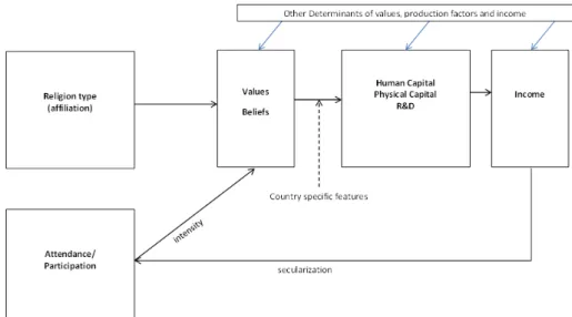
From the literature, I can construct a simple diagrammatic model to explain the relationship between religion and income (see Figure 3.1). The diagram highlights that religions act on in-come through the values they shape. The values depend on the religion (e.g. Catholics believe that rewards from a pious life will be obtained in Heaven while Protestants believe that success on Earth is a sign of God’s approval) but the intensity with which the values are felt depends on the participation individuals have in religion, and that participation is proxied by attendance to religious activities. Empirical studies have used both church membership and participation as determinants of income, and these have yielded different results. Values and beliefs may have the ability to influence the accumulation of production factors (human and physical capital), thereby affecting the work capacity of individuals and the desire for sucsess, and also affecting the entrepre-neurial ability, which may influence new ideas and innovation. However, beliefs and values may be influenced by determinants other than religion type and attendance. Examples of these (omitted) variables in the relationship between religion and beliefs may be related to meteorology (e.g. a natural disater may be interpreted as a sign of God’s punishment for sins) or institutional change in some religion (e.g. the election of a new pope, religions schisms). As the same religion is common to (many) different countries, these (omitted) variables influencing religious beliefs may often be common to different countries. Determinants of factors of production and income include features such as policies, institutions and preferences. This relationship between religion and income is therefore crucially affected by omitted variables. However, income also influences participation or attendance in religious activities, in a phenomenon called secularization. In fact, as income grows due to education or technological progress, religious attendance tends to fall. This potential reverse effect has to be taken into account in order to avoid biased estimations.
My empirical approach is robust to the issues of omitted variables and causality highlighted in Figure 3.1. The fact that country-specific culture may incorporate a common religion in specific ways may determine that the effect of religion on country income is specific to each country. In particular, the empirical strategy used in this chapter is also robust to heterogeneity between different countries and to the fact that the relationship between religion and income may be hit by factors that are common to diverse countries.
3.2 Empirical Relationship between Religion and Income
In this section I present the empirical relationship between religious participation and income. First I present the data and sources (Section 3.2.1). Then I detail the empirical method (Section 3.2.2). Sections 3.2.3 and 3.2.4 presents the results of estimation.
3.2.1 Data and Sources
The data on religious attendance are based mostly on surveys specific to one or several coun-tries. A complete panel data for religious attendence become available with Iannaccone (2003), who provided a dataset on religious attendence in 32 countries from 1925 to 1990.2 The idea of
Iannaccone’s study was to estimate historical church attendance rates using contemporary ISSP (International Social Survey Programme) questionnaires and replies to inquires on church atten-dance when the respondents were 11 or 12 years old. The survey asked the following questions: "1) When you were around 11 or 12, how often did you attend religious services then? 2) When you were a child, how often did your father attend religious services? 3) When you were a child, how often did your mother attend to religious services?". Naturally, this retrospective method could be impaired by carious biases (e.g. social desirability, conventional wisdom, age effects, or projection bias). Iannaccone the devotes the greater part of his study to carefully demonstrate that there is no reason for concern. As examples, a uniform social desirability bias will inflate overall measures of church attendance but not distort its trends, turning points, or the qualitative relationships between attendance and its correlates. According to the author, the most extreme biases tend to preserve national rankings and other cross-country comparisons of religious activity. On the other hand, retrospective data may actually be more accurate than non-retrospective data. This is almost certainly true throughout Eastern Europe and the former Soviet Union, where before the collapse of communism religious people had good reason to understate their religiosity. And even in the United States and western Europe, where standard surveys cover many decades, re-trospective data provide an alternative view of the past when compared to standard surveys. This is important given the possibility that replies to standard survey questions have shifted over time due to changing social pressures, looser interpretations of questions, or declining response rates. Advantages of these data include availability of long series of data per country and consistency across time periods.
For variables other than religion attendance I use the Penn World Tables 8.0. As I wish to model the relationship between income and religion my basic framework is the neoclassic production function, and I thus use GDP per capita (at constant national prices (in mil. 2005 USD))3 and
the capital stock at constant national prices (in mil. 2005 USD) per capita. In some specifications I also use human capital (Index of human capital per person, based on years of schooling (Barro
2The countries in Iannaccone’s database are: Australia, Austria, Bulgaria, Canada, Chile, Cyprus,
Czech Republic, Denmark, France, West Germany, East Germany, Great Britain, Hungary, Ireland, Italy, Japan, Latvia, Netherlands, New Zealand, Northern Ireland, Norway, Philippines, Poland, Portugal, Rus-sia, Slovakia, Slovenia, Spain, Sweden, Switzerland and United States. I disregard Northern Ireland in the empirical exercise and construct a population-weighted average of the measures of West and East Germany to match Germany in the empirical exercise. Although originally this source supplies data at five-year in-terval, I have linearly extrapolated within at five-years interval to obtain yearly observations between 1925 and 1990. This procedure was also used the PWT 8.0 to construct the human capital variable.
3I present alternative measures of per capita GDP to check for robustness of results. Alternative
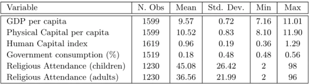
and Lee, 2013) and returns to education (Psacharopoulos, 1994) ) and the share of government consumption (at current PPPs) from the same source. Descriptive statistics are presented in Table 3.1.
Tabela 3.1: Descriptive Statistics
Variable N. Obs Mean Std. Dev. Min Max
GDP per capita 1599 9.57 0.72 7.16 11.01
Physical Capital per capita 1599 10.52 0.83 8.10 11.90
Human Capital index 1619 0.96 0.19 0.36 1.29
Government consumption (%) 1519 0.18 0.48 0.48 0.56
Religious Attendance (children) 1230 45.08 26.42 2 98
Religious Attendance (adults) 1230 36.56 21.99 2 96
Notes: Output per capita, physical capital per capita and human capital are in natural logarithms.
3.2.2 Estimation and Methods
Heterogeneity and cross-section dependence in macro data have been extensively documented in very recent research (see a survey in Eberhardt and Teal, 2011 and a empirical applications in Eberhardt and Teal, 2013a, 2013b and Eberhardt and Presbitero, 2014). Here I document hetero-geneity in religion attendance. Figure 3.3 is clear about different patterns of religious attendance across countries and also seems to indicate non-stationarity of these variables, which was also documented in Dierk and Strulik (2013). Table 3.2 presents results of the cross-sectional depen-dence test of Pesaran (2004) and of the Pesaran (2007) unit-root test which clearly reject the null for no cross-section dependence and do not reject the null for a unit-root (exception for religious attendance - adults), whitch invalidate traditional approaches for panel data econometrics. As Eberhardt and Teal (2011) put it, "The standard empirical estimators (e.g. fixed effects, difference and system GMM) not only impose homogeneous production technology, but they also implicitly assume stationatiry, cross-sectionally independent, variables". In fact, most of macroeconomic data do not fulfill those assumptions and those estimators are therefore not appropriate for studying growth regressions (as I do in this study). I will use the Pesaran (2006) common correlated effects mean group estimator to address my empirical objective.4 One of the important features of this
estimator in comparison to other panel data estimators is that it is robust to country-fixed effects such as geography, culture and initial religion-related beliefs , and to unobservable common vari-ables such as common productivity change (TFP), the common evolution of religious thinking or events to which beliefs within countries may react differently.5 Moreover, this estimator is also
robust to the presence of stationary and non-stationary regressors.
4Advantages and robustness of this class of heterogeneous estimators over traditional fixed-effects and
instrumental variables panel estimators is documented in Eberhardt and Teal, 2011.
5This is consistent with initial country specific beliefs that evolve differently in each country due to
common factors which affects religions as a whole (e.g. the Second Vatican council; the election of new popes; the increase of new cults or sects; the proclamation of a new Saint) or other common factors such as the technological progress, ICT diffusion, and/or globalization.
Figura 3.2: Religion (children) Attendance by Country, 1925-1990 0 50 10 0 0 50 10 0 0 50 10 0 0 50 10 0 0 50 10 0 1950 1960 1970 1980 1990 1950 1960 1970 1980 1990 1950 1960 1970 1980 1990 1950 1960 1970 1980 1990 1950 1960 1970 1980 1990 1950 1960 1970 1980 1990
Australia Austria Bulgaria Canada Chile Cyprus
Czech Republic Denmark France Germany Great Britain Hungary
Ireland Israel Italy Japan Latvia Netherlands
New Zealand Norway Philippines Poland Portugal Russia
Slovakia Slovenia Spain Sweden Switzerland United States
Re lig io us A tte nd an ce (c hi ld re n) Year
Figura 3.3: Religion Attendance by Country, 1925-1990
0 50 10 0 0 50 10 0 0 50 10 0 0 50 10 0 0 50 10 0 1950 1960 1970 1980 1990 1950 1960 1970 1980 1990 1950 1960 1970 1980 1990 1950 1960 1970 1980 1990 1950 1960 1970 1980 1990 1950 1960 1970 1980 1990
Australia Austria Bulgaria Canada Chile Cyprus
Czech Republic Denmark France Germany Great Britain Hungary
Ireland Israel Italy Japan Latvia Netherlands
New Zealand Norway Philippines Poland Portugal Russia
Slovakia Slovenia Spain Sweden Switzerland United States
Re lig io us A tte nd an ce (A du lts ) Year
The basic equation of interest in my analysis of the religion-income relationship is the following neoclassical production function augmented with religious attendance:
yit= β1ikit+ β2iRit+ uit; uit= αi+ λ0ift+ εit , (3.1)
where y is the natural logarithm of per capita GDP, k is the log of the stock of physical capital per capita, R is religious attendance as defined above, ft is the vector of unobservable common
factors and λ0
i is the associated vector of factor loadings, αi are country-fixed effects and εit is
the error term. As can be observed from (3.1), each coefficient is country-specific, thus allowing for complete heterogeneity in the estimation. Additionally, as each regressor can also depend on the common factor, the method is also robust to endogeneity of the observable factors toward the common factors. In some specifications, I will also add to the regression in (3.1) human capital and government consumption expenditures as a share of GDP. Because of the semi-log specification, the coefficient β2 has a straightforward interpretation: it is the economic growth rate obtained
from a variation in attendance in 1 percentage point.6
Tabela 3.2: Cross-Sectional Dependence and Unit Root Tests
(1) (2) (3) (4)
Variable GDP per capita Physical Capital
per capita Religious Attendance (children) Religious Attendance (adults) CD T est 127.92*** 132.30*** 81.96*** 79.00*** (p-value) (0.000) (0.000) (0.000) (0.000)
Unit Root Test -0.986 3.544 0.625 -3.084***
(p-value) (0.162) (1.000) (0.734) (0.001)
Note: Level of significance: *** for p-value<0.01; **for p-value<0.05;* for p-value<0.1. Output per capita and human capital are in natural logarithms. The cross-sectional dependence test is the Pesaran (2004) test under the null of no cross-section dependence. The unit root test
is the Pesaran (2007) test with one lag and no trend which tests the null of I(1) series.
Given the importance of time series properties and dynamics in macro panel analysis, I employ an error correction model (ECM) representation of the above equation.7 This offers at least four
advantages over a static model such as the above or restricted dynamic specifications such as those commonly investigated in the growth-regressions literature: (i) I can readily distinguish short-run from long-run behaviour; (ii) I can investigate the error correction term and deduce the speed of adjustment for the economy to the long-run equilibrium; (iii) I can test for cointegration in the ECM by closer investigation of the statistical significance of the error correction term, and (iv) once cointegration is proven, I can conclude for a Granger-causal effects of the right-hand side variables on income. It is particularly important that the effect of religion obtained on income can be assumed to be robust to reverse causality. However, the analysis of an eventual reverse causation from income to religion is beyond the scope of this paper. The ECM representation of the above model is as follows:
Δyit= αi+ ρi(yit−1− β1ikit−1− β2iRit−1− λ0ift−1) + γ1iΔkit+ γ2iΔRit+ γ3iΔft+ uit, (3.2)
where βjirepresent the long-run equilibrium relationship between GDP and the measures of
phy-6I also tested log-log specifications in Religion attendance and my conclusions are not affected by this
specification choice.
7This is an approach also followed in Eberhardt and Prebistero (2014) to study the effect of public debt
sical capital and religion while represent the short-run relationship between capital and religion on one side and GDP in the other side. From the regression results long-run coefficients βji can
be recovered dividing the coefficients obtained by ρi. Following Pesaran (2006) and Banerjee and
Carrion-i-Silvestre (2011) I add to eq. (3.2) cross-section averages of all variables in the model (GDP per capita; physical capital per capita and religion attendance) to replace unobservables as well as omitted elements of the cointegration relationship. However, as shown in Chudik and Pesaran (2013), this approach is subject to small sample bias, especially in panels with time-series of moderate dimensions, as is this case. Chudik and Pesaran (2013) offer an empirical strategy to deal with weakly exogenous regressors, whitch is thus robust to reverse feedback (from income to religion in this case). They suggest, in addition to the cross-section averages mentioned above, the inclusion of further lags of the cross-section averages.
p X l=1 τjilΔyt−p+ p X l=1 τjilΔkt−p+ p X l=1 τjilΔRt−p. (3.3)
I follow Chudik and Pesaran (2013) rule of thumb to choose the number of lags to be introduced (p = T1/3). Thus with a time series of between 35 and 56 years on average, the rule of thumb
indicates a value between 3 and 4. In my ECM this equates to adding up to two to three lagged differences. I include three lagged differences in my regressions.8
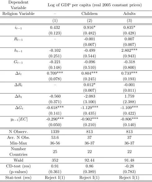
3.2.3 Results
In this section I present the results of the estimation of equation (3.2) and some extended versions of it. Table 3.3 shows the main results. The first three columns present the results of estimation of the baseline equation 3.2, beginning with a regression in which religion does not enter (column 1) and then presenting two other regressions in which religion enters (as children attendance and adult attendance, respectively). The table also presents results for enlarged regressions in which human capital and government consumption enter, following the same scheme (the first regression without religion attendance and then the other two, with religion attendance).9
I can now analyse results in the Table. For all models there is evidence of error correction and the coefficient on the lagged GDP per capita is highly significant and shows reasonable estimates for spead of convergence. Half-life estimates range from 0.1 to 2.2 years, values which are similar to those in Eberhardt and Prebistero (2014).10 The presence of religion in regressions clearly shrinks
the time of convergence. The simple estimation in column (1) is an estimation of a neoclassical production function in an Error-Correction Model (ECM) form. This yields statistical significant effects of physical capital in both the short and long-run. As mentioned earlier I can retrieve the long-run parameters dividing the long-run estimated coefficients by the error-correction coefficient. Thus, column (1) yields a long-run physical capital share of 0.39, also consistent with empirical evidence. Columns (2) and (3) enlarge the equation for inclusion of religion, maintaining the high significance of both long and short-run effects of physical capital (with an implied long-run share
8An alternative choice of two lags would not change my results. Results with two lags are available
upon request.
9I choose to estimate those regressions without a country-specific trend because when testing results
with a trend, changes in results are minor and trends are not statistically significant.
10Half-life is the length of time after a shock before the deviation in output shrinks to half of its impact
of physical capital of 0.26 to 0.45, thus within quite reasonable values). The effects of religion are clearly non-significant in both the long and short run.
Now, column (4) represents an enlarged production function which includes typical determinants of economic growth from the growth regressions à la Barro literature: the human capital index and the government consumption share in GDP. The results in column (4) yield only short-run significant results of physical capital and a negative effect of government consumption which is consistent with the majority of the empirical literature on economic growth. Column (5) maintains the short-run negative and significant effect of government consumption share and column (6) maintains the short-run positive and significant effect of per capita physical capital. Both columns (5) and (6) show non-significant effects of religious attendance. Non-significant averaged results for religion do not dismiss à priori significant country effects. I investigate this possibility and report in the Table 3.3 the number of countries with significant results. I in fact conclude that only a minority of countries (a maximum of 6 out of 22 that enter in the regressions with religion) appear with significant effects of religion in the short and long run and positive and negative significant coefficients are quite balanced. For example, in column (2) I found one country with long-run positive effect and another with long-run negative effect of religion. Additionally in the short run, I found four countries with significant positive effect and three countries with significant negative effects. The fact that overall I found non-significant effects of religious attendance on economic growth is indeed important to the understanding of growth performance of the respective country. This is also a contrbution to the empirical discussion on the relationship between religion and growth, in which, once reverse causality and heterogenity between countries are taken into consideration, the effect turns out to be negligible.
3.2.4 Robustness
I perform a number of robustness checks in order to see if religion’s non-significant result is depen-dent on the specific variables that are used in my benchmark model, although I use a benchmark specification for production function which yields my model in equation (3.1).
First, I change the dependent variable to other definitions of real GDP that are available in the PWT 8.0, expenditure-side real GDP at chained PPP’s (Purchase Power Parity) and output-side real GDP at chained PPP’s. There are no important changes when changing the definition of the dependent variable except for some decrease in the statistical significance of the long-run coefficient of physical capital in the reduced form regressions similar to those in columns (1) and (2) of Table 3.3.11
Second, I change the variable that measures the contribution of physical capital to income. Fol-lowing more closely the growth regressions literature à la Barro, I use the share of investment in GDP to account for the effect of physical capital in extended regressions similar to those of columns (4) to (6) of Table 3.3. Interestingly, now more variables are significant in the long run. Adding to the investment share, which is significant in both the short and in the long run, in the regression similar to that in column (6) of Table 3.3 I also obtain a positive long-run coefficient for human capital, which is consistent with most empirical literature on economic growth and human capital. The government consumption share is always highly significant (with a negative sign) in the short run. On these regressions I obtain only one statistically significant sign of religious attendance (of
children) coefficient in the short run (p-value=0.078).12
Tabela 3.3: Income and Religion in Heterogeneous Panels Dependent
Variable Log of GDP per capita (real 2005 constant prices)
Religion
Variable – Children Adults – Children Adults
(1) (2) (3) (4) (5) (6) kt−1 0.103** 0.184* 0.331** 0.041 -0.285 0.238 (0.041) (0.105) (0.138) (0.081) (0.384) (0.299) Rt−1 – -0.001 0.001 – -0.013 0.003 (0.002) (0.001) (0.008) (0.007) ht−1 – – – 0.058 -1.605 -1.457 (0.264) (1.053) (1.188) Gt−1 – – – -0.198 0.061 -0.359 (0.173) (0.960) (0.860) Δkt 1.527*** 2.276*** 2.386*** 1.720*** 0.756 1.933*** (0.174) (0.192) (0.237) (0.218) (0.565) (0.298) ΔRt – 0.002 0.005 – -0.001 0.002 (0.005) (0.005) (0.010) (0.006) Δht – – – 0.566 2.149 -0.936 (0.420) (1.599) (1.797) ΔGt – – – -0.686*** -1.419** -0.622 (0.163) (0.568) (0.472) yt−1[EC] -0.266*** -0.702*** -0.729*** -0.490*** -0.721*** -0.999*** (0.029) (0.041) (0.045) (0.042) (0.194) (0.095) N Observ. 1479 813 813 1389 813 813 Avr. N Obs. 49.3 37 37 55.6 37 37 Min-Max 18-58 36-37 36-37 38-58 36-37 36-37 Number Countries 30 22 22 25 22 22 Wald 257*** 602*** 468*** 302*** 96*** 180*** CD-test (res) 2.84*** 1.65* 2.84*** 0.83 0.49 2.37** (p-values) (0.005) (0.099) (0.005) (0.404) (0.625) (0.018)
Stat-test (res) Reject I(1) Reject I(1) Reject I(1) Reject I(1) Reject I(1) Reject I(1) sig. signs /countries for R (LR) – (1)(1) (4)(0) – (5)(6) (1)(4) sig. signs /countries for R(SR) – (4)(3) (2)(1) – (3)(4) (3)(3)
Note: Dependent Variables natural logarithm of the GDP. A constant is included in the regressions but omitted from the Table. Values between parentheses below coefficients are robust (clustered) standard errors. Level of significance: *** for p-value<0.01; **for p-value<0.05;* for p-value<0.1. Wald test is a joint significance test for the regressors. CD-test is a Pesaran (2004) cross-section dependence test on the null of cross-section independence done on the residuals from the regression (p-value presented between parentheses). Stat-test is the Pesaran (2007) unit root test made on the residuals. This test used 1 lags and rejects I(1) means that in all lags the test of unit root
rejects. The list of countries that enter in regressions with religion are provided in the Appendix A.6.