D. T. Seaton, S. J. Mitchell, and D. P. Landau
Center for Simulational Physics, University of Georgia, Athens, GA 30602, USA
Received on 17 October, 2007
The Wang-Landau method is used to study thermodynamic properties of a three-dimensional flexible ho-mopolymer chain with continuous monomer positions. Results describing the coil-globule and solid-liquid transitions are presented for chain lengths up toN=100. In order to elucidate the thermodynamic behavior, finite chain length effects and the influence of the energy range over which the density of states is determined are carefully analyzed. Simulation efficiency is also studied and it is shown that setting the natural logarithm of the final modification factor equal to 10−6is an appropriate choice for this model.
Keywords: Homopolymer chain; Wang-Landau method; Coil-globule transition; Solid-liquid transition
I. INTRODUCTION
Polymer systems have provoked much interest in an ar-ray of different disciplines, and in recent decades computer simulations have become powerful and mature. In particular, Monte Carlo methods [1] have shown great promise in the in-vestigation of thermodynamic properties of these systems [2]. However, traditional Monte Carlo methods have had trouble sampling the rough energy landscapes associated with some polymer models. The Wang-Landau method [3–5] has proven quite useful in overcoming these inefficiencies. Since the tar-get of our current study is understanding the behavior of a flexible homopolymer when the temperature is lowered and multiple states begin to compete, Wang-Landau sampling is very well suited for this problem.
In two recent studies, the Wang-Landau method was used to investigate the phase behavior of two related models for a single homopolymer. Rampf et al. [6–8] used the bond-fluctuation model [9] to study single chain properties, while Parsons and Williams [10, 11] used a continuous homopoly-mer model. Both models had simple interaction potentials and both studies found coil-globule and solid-liquid transitions. The coil-globule transition [12] represents the change from an unwound, random coil, to a more compact, globular state. The solid-liquid transition is the collapse of the polymer from a compact globular state into a nearly frozen, “crystalline” state. Representative configurations for these states are shown in Fig. 1. Additionally, these studies [6–8, 10, 11] provide some evidence of intermediate states for large chain lengths. Parsons and Williams also made comparisons between their results and the results from Rampf et al., highlighting differ-ences between the two models. These differdiffer-ences were orig-inally quite dramatic, but recent work from Rampf et al. [8] shows that by increasing the interaction distance of their non-bonded potential, the coil-globule and solid-liquid transitions behave more like those in the Parsons and Williams study. Nonetheless, the two studies still show significant differences in their thermodynamic behavior.
The aim of the work in this article is to understand the be-havior of a simple continuous homopolymer, while also mak-ing comparisons to the results found in the previously dis-cussed studies [6–8, 10, 11]. The results reported here show conflicting conclusions compared with the continuum model
results from Parsons and Williams. The nature of the solid-liquid and the coil-globule transitions appear to be different, even though the models are nearly identical. In order to un-derstand these differences, the work presented here focuses on making a systematic study of a single continuous homopoly-mer using Wang-Landau sampling.
II. MODEL
The polymer model we consider consists of a chain of N identical monomers, where each monomer position may vary continuously in three-dimensional space. There are two types of interactions: a bonded interaction between nearest-neighbor monomers and a non-bonded interaction between non-bonded monomers. The Hamiltonian for this model is
H
=N−1
∑
i=1UBond(li) +
∑
i,jULJ(ri j), (1)
where the first term represents the bonded energy, summed over all N−1 bonds using the bond potential UBond(li), which is a combination of a finitely extensible nonlinear elas-tic (FENE) potential [2, 13] and a Lennard-Jones potential. The second term in
H
represents the non-bonded energy, summed over all interactions between non-bonded monomer pairs (i,j), whereULJ(ri j)is a Lennard-Jones potential, and ri jis the distance between two non-bonded monomers. The Lennard-Jones potential is given byULJ(ri j) =
4ε
σ ri j
12
−
σ ri j
6
, for 0<ri j≤3σ,
0, otherwise,
(2) where the subscripti jrepresents ani-jpair,ri jis the distance between these two monomers,εis the well depth, andσis the distance at which the potential function is a minimum. Di-mensionless units are used, whereε=1 andσ=2−1/6, and the minimum is then located atri j=1.
The FENE potential is given by
UBond(li) =
0.5kR2oln[1−(li/Ro)2], forli<Ro,
Globule
Random Coil
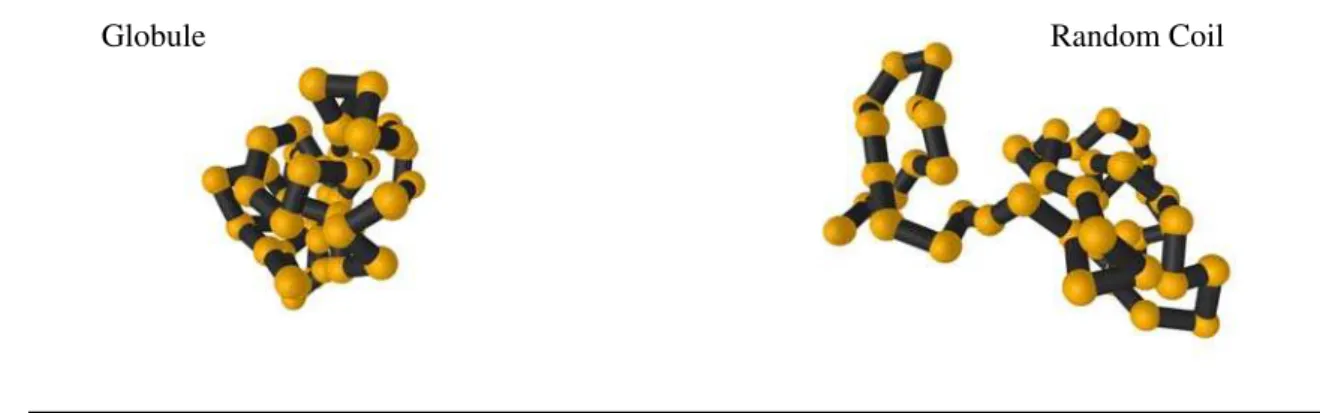
FIG. 1: Two configurations are shown for a chain length ofN=50: the left representing a globule and the right representing a random coil. These configurations were taken from a single Wang-Landau simulation, where configurations were saved for particular energy values. These two configurations are general representative states found near the coil-globule transition.
0.75 1 1.25 1.5 1.75 2
r
-10 1 2 3 4
U(r)
Non-Bonded Potential Bonded Potential
FIG. 2: Plot showing both the bonded and non-bonded poten-tials. The non-bonded function is a Lennard-Jones potential and the bonded function is a combination of a FENE and the same Lennard-Jones potential.
whereRois the finite extensibility and is set toRo=1.2,kis the stiffness constant and is set tok=2,liis the bond length and has an equilibrium distance oflo=1. All parameters were chosen such that the minima of bothUBond(l
i)andULJ(ri j)are at a distance of 1. For comparison, the FENE and Lennard-Jones potentials are plotted in Fig. 2.
III. METHOD
Wang-Landau sampling is a Monte Carlo technique that was developed as a temperature independent, iterative method with the ability to sample rough energy landscapes [5, 14]. The technique was originally implemented for discrete models [3], and in order to perform simulations of a continuous model a few issues must be addressed. (Recent work has focused on
optimizing the Wang-Landau method for continuous systems [15, 16]; the implementation for this study was directed at un-derstanding the effects of finite length and restricted energy range for the random walkers, so an implementation close to the original method was adopted.)
The Wang-Landau sampling approach is based on calculat-ing the density of statesg(E), whereE is the energy of the system. An initial estimate of the density of statesg(E) =1.0 is made. The algorithm proceeds by generating trial states, us-ing appropriate “moves”, and acceptus-ing them with transition probability
p(Ei→Ef) =min g(Ei) g(Ef)
,1
, (4)
whereEiis the initial energy andEf is the energy of the trial state. If the trial move is accepted, the density of states is mul-tiplied by a modification factorf, i.e.g(Ef)→g(Ef)×f, and a histogramH(E)is also updated,H(Ef)→H(Ef) +1. If the trial state is rejected, the same procedure is followed for the initial energyEi. This process is repeated until the histogram H(E)is sufficiently flat, at which point the histogram is reset to zero, the modification factor is reduced by f →√f, and the random walk continues. The initial value of the modifi-cation factor is set to f =e1and is eventually reduced to a value which is ff inal≈1. The flatness ofH(E)is defined as its minimum divided by its average, and in this study, the flat-ness criterion is set to 0.8. Becauseg(E)becomes extremely large in the actual computation, the logarithm of the density of states,ln[g(E)], is used to prevent overflow during the actual simulation. More details about Wang-Landau sampling can be found elsewhere [5, 14].
-4 -3 -2 -1 0
E / N
-500 -400 -300 -200 -100
ln[g(E)]
N = 10 N = 25 N = 50 N = 100
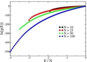
FIG. 3: Density of states for chain lengthsN=10, 25, 50, and 100, where the energy range varies for each chain length and the maxi-mum of each function is normalized to zero. Each point is the av-erage of 10 independent simulations (error bars are smaller than the size of the symbol).
report will be the foundation for future work, so the simplest approach was implemented by first establishing a lower and upper bound for the Wang-Landau method to sample. (The choice of a lower energy bound is important because with too low a value the histogram never becomes sufficiently flat.) In some continuous models the ground state energy is not known, and the value of the upper energy bound, beyond which con-tributions to the behavior near any polymer collapse are small, may also not be well known. In this study, simulations have been performed over a number of different energy ranges in order to determine how they affect the thermodynamic prop-erties.
Once an energy range has been defined, the energy is di-vided into a discrete number of bins, which defines the bin-ning resolution. Testing showed that a bin resolution of dE =0.1 was generally a good choice. The only exception being for the chain length ofN=100, wheredE=0.2 was used to prevent the number of bins from becoming too large. (For example, forN=100, a resolution ofdE=0.1 and an energy range ofE/N= [−4.0,3.0]requires 7000 bins.) Since the effects of bin resolution have still not been well studied, attempts were made to keep the number of bins reasonably low for computational efficiency.
In each simulation the chain starts from a straight config-uration. Changes are made to the polymer configurations us-ing the followus-ing types of trial moves: sus-ingle monomer dis-placement (“diffusion”), reptation, crank-shaft, and random pivot. One Monte Carlo sweep (MCS) consists of N attempted monomer displacement moves and a single attempt of each of the other types of moves. The moves are identical to those de-scribed in reference [18]. It is also important to note that an at-tempt was made to locate the approximate ground state energy for each chain length, insuring that the energy ranges used were reasonably appropriate in each simulation. This was done by simply allowing the Wang-Landau method to sam-ple a large energy space with a small bin-resolution.
Wang-0.2 0.3 0.4 0.5 0.6 T
1.6 1.8 2 2.2 2.4 2.6
CV
/ N
0 0.5 1 1.5 2 2.5 3
T
0 0.5 1 1.5 2 2.5
C V
/ N
Emin/N = -1.7 Emin/N = -1.5
FIG. 4: Specific heat versus temperature for a chain length ofN=
10, for three different minimum energy boundaries,Emin/N=−1.5,
−1.7, and−1.9. The maximum energy boundary is set toEmax/N=
0.0 for all of the curves. Each point is the average of 10 independent simulations (error bars are smaller than the size of the symbol).
Landau sampling has the ability to be optimized to find ground states in various systems[15], but in this work, only testing was performed and only approximate ground state energies are reported.
IV. SIMULATION RESULTS
In all figures that follow, data points represent averages over 10 or more independent runs. Fig. 3 shows the density of states for four different chain lengths: N=10, 25, 50, and 100, where the maximum of each function has been normal-ized to ln(g(E)) =0. The range of g(E)increases rapidly with chain length, and the dependence upon energy becomes particularly important at low energies. These are the results from early simulations where it was still unclear what the en-ergy range should be for different chain lengths. Each data set is shown over a distinct energy range, where the minimum energy boundary, Emin/N, varies with chain length, but the maximum energy boundary is fixed atEmax/N=0.0 for all chain lengths. The maximum energy was initially set to zero based on the work from Rampf et al. [6–8] and Parsons and Williams [10, 11]. The minimum energy was “pushed” as low as it was possible to simulate efficiently, i.e. with a maximum run time of 10 days.
A. Effect of Energy Boundaries
0 0.5 1 1.5 2 2.5 3
T
0 0.5 1 1.5 2 2.5 3
C V
/ N
Emax/N = 0.0 Emax/N = 1.0 Emax/N = 2.0 Emax/N = 3.0
2.5 2.6 2.7 2.8 2.9 3 T
0 0.1 0.2 0.3
CV
/ N
FIG. 5: Specific heat versus temperature for a chain length ofN=10, for three different maximum energy boundaries,Emax/N= 0.0, 1.0,
2.0, and 3.0. The minimum energy boundary is set toEmin/N=−1.9
for all of the curves. Each point is the average of 10 independent simulations (error bars are smaller than the size of the symbol).
single rounded peak at approximatelyT ≈0.5. As the mini-mum energy is lowered, noticeable differences in the specific heat appear. The curve withEmin/N=−1.7 begins to show two interesting features, a taller peak and a shoulder. As the energy boundary is lowered toEmin/N=−1.9, a clear peak appears atT ≈0.2, while the shoulder remains at T ≈0.5. These results usingN=10 show how dramatically the min-imum energy boundary can affect thermodynamic quantities. This chain length allowed the minimum energy to be pushed very close to the ground state with,Egs≈ −1.93.
The maximum energy boundary can also affect thermody-namic quantities more substantially than might be expected. In Fig. 5, the maximum energy boundary is varied for a chain length ofN=10. Each of the four curves in this plot has a minimum energy ofEmin/N=−1.9, which is the lowest en-ergy boundary from the previous graph, Fig. 4. Each set of data points represents a different maximum energy boundary, Emax/N=0.0, 1.0, 2.0, and 3.0. ChangingEmax/Ndoes not affect the specific heat at low temperatures, but does affect the quantity at higher temperatures. The shoulder seen in Fig. 4 has now been stretched out slightly, compared to the curve withEmax/N=0.0. The three curves with larger values for this boundary have smaller, but still noticeable, differences. The inset in Fig. 5 gives a better view of these differences at higherT. Metropolis sampling was also performed for the temperature range in the inset, and the results of these simu-lations agreed with the data from theEmax/N=3.0 curve to within the respective error bars.
B. Chain Length and Transitions
The results for the small chain length shown in the previ-ous figures illustrate some of the issues one must deal with when performing Wang-Landau simulations on this type of model. Once these features were better understood, larger
0 0.5 1 1.5 2 2.5 3
T
02 4 6 8
C
V/ N
N = 10 N = 25 N = 50 N = 100
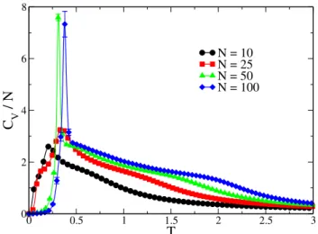
FIG. 6: Specific heat versus temperature for chain lengthsN=10, 25, 50, and 100. Two distinct features can be seen: the solid-liquid transition at low temperature, and the coil-globule transition at higher temperatures. Each point is the average of 10 independent simula-tions (where most error bars are smaller than the size of the symbol).
chain lengths were simulated, where similar energy range studies were performed for each chain length. In Fig. 6, the specific heat is plotted versus temperature for four different chain lengths, N =10, 25, 50, and 100. The two features which became apparent while varying the minimum energy boundary are now very different. The small peak noticed for N=10 has become quite sharp for larger lengths, suggesting that a first-order transition might occur in the thermodynamic limit of infinite chain length, and the small shoulder has now been stretched out to even higher temperatures, indicating an even broader ’intermediate’ region. TheN=100 curve dis-plays two prominent features. The first is the low-temperature peak atT ≈0.4, which is believed to represent a solid-liquid transition. The second feature is the coil-globule transition which is represented by the shoulder atT≈2.0. Recent work with larger chain lengths [8, 11] has also shown that the area in between these transitions can contain other interesting meta-stable states; however, for the chain lengths presented above, such features were not observed. Simulations of larger chain lengths, accompanied by rigorous structural analyses, are still needed to better understand all of these interesting regions.
Note that in Fig. 6, the energy ranges for the respective ln[g(E)]have been adjusted to follow the results seen in the previous figures. e.g., forN=100, the energy range isE/N= [−4.0,3.0]. Emax/N=3.0 for all of the chain lengths, while Emin/Nare the same for the chain lengths given in Fig. 4.
C. Simulation Efficiency and the Modification Factor
-4 -3 -2 -1 0 1 2 3
E / N
-300 -250 -200 -150 -100 -50 0
ln[g(E)]
N = 10 N = 25 N = 50
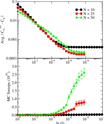
FIG. 7: Average density of states calculated for three different chain lengths,N=10, 25, and 50. Each point is the average of 50 indepen-dent runs and the error bars are much smaller than the symbol size. These curves are used to create reference thermodynamic quantities, and these quantities are used to study the efficiency of the simula-tions.
original study on discrete spin models [3] used a final value of ln[f] =10−8; but in most of the recent work on polymer models, a final modification factor ofln[f] =10−6was used. The aim of this section is to better understand why 10−6is an appropriate choice for this model.
In order to resolve whether the selection ofln[fmin] =10−6 made in some studies was warranted, 50 independent runs were made for each of the following chain lengths: N=10, 25, and 50. In each run, g(E)was recorded for each value of the modification factor, i.e. at the completion of each level of iteration. The final value of ln[f]was reduced to at least ln[fmin] =10−8, and the final values ofln[g(E)]were aver-aged together. In Fig. 7, the average values of ln[g(E)]are plotted as a function of energy for each of the chain lengths. The energy ranges follow the same criterion described in the previous section regarding energy boundaries, where the max-imum and minmax-imum cutoffs have been extended far enough to insure that the important thermodynamic features are re-produced correctly. Using these average values ofln[g(E)], a reference value of the specific heat,CVre f, is calculated for each chain length. These values will now serve as a ref-erence which will be compared to specific heat curves cal-culated from the ln[g(E)] values at each iteration level of ln[f]. When comparing the reference with specific heat curves calculated at a particular value of ln[f], the absolute differ-ences,
C
re f
V (T)−CV(T)
, are then averaged and stored for
each value ofln[f]. These difference values, for eachln[f], are then averaged for all 50 independent runs and error bars are calculated.
The top of Fig. 8 shows the absolute difference between CVre f and the calculatedCV for each value ofln[f], and the bottom of Fig. 8 shows the average number of MC sweeps versusln[f]. The same 50 independent runs for each chain length were used to produce the curves in both plots. The top
10-8
10-6
10-4
10-2
0.0001 0.001 0.01
Avg. | C
V
ref - C
V
|
N = 10 N = 25 N = 50
10-10
10-8
10-6
10-4
10-2
100
ln (f) 0.0
0.5 1.0 1.5 2.0 2.5 3.0
MC Sweeps (10
10 )
FIG. 8: Top: average absolute difference in the specific heat between the reference curve and single iterations ofln[g(E)]versus tion factor. Bottom: average number of MC sweeps versus modifica-tion factor, where these data come from the same independent runs used in the top plot. A total of 50 independent runs were performed for each chain length.
plot shows how the error decreases during the course of a sim-ulation. For theN=10 system length, the curve decreases as ln[f]decreases, but then levels off atln[f]≈10−6. The simu-lations for this system size were continued to a final value of the modification factor ofln[f] =10−10, and it is clear that any extra time spent running a single simulation pastln[f]≈10−6 does not necessarily improve the final result (at least for our choice of flatness criterion). The other two chain lengths plot-ted were simulaplot-ted to a value ofln[f] =10−8. Again, the aver-age deviation levels off atln[f]≈10−6. However, the bottom plot reveals that a huge price is payed in terms of the number of MC sweeps needed to iterateln[f]from 10−6to 10−8. For N=25, the number of MC sweeps executed afterln[f] =10−6 is twice the number executed beforeln[f] =10−6. ForN=50 we observe a similar behavior, only the number of sweeps needed to reach ln[f] =10−8 is nearly 3 times larger than the number needed to reachln[f] =10−6. Thus, when con-sidering both efficiencyandthe error associated with Wang-Landau simulations, we find thatln[fmin] =10−6is a very rea-sonable choice.
V. CONCLUSIONS
N =100. It was found that the energy range used by the Wang-Landau random walk can dramatically affect the shape of the specific heat. For instance, the solid-liquid transition can be easily hidden if the minimum energy is too high. Along those same lines, if the maximum energy boundary is too low, the specific heat at higher temperatures indicates too low a coil-globule transition temperature. (Although not shown in this article, similar effects are seen in other thermodynamic quantities.) We also find that a final value of the modification factor equal toln[f] =10−6is appropriate, given our choice of flatness criterion (0.8), and iterating to a still lower value only increases the CPU time with very little improvement in the final results.
The results presented here differ considerably from those reported by Parsons and Williams [10, 11], even though the models used are nearly identical. Interestingly, our results tend to have many more similarities with the work from Rampf et al. [6–8] using the bond fluctuation model, espe-cially with regards to the their latest work [8]. This is partic-ularly true for the solid-liquid transition, where a sharp peak in the specific heat is seen at low temperature. The exact val-ues of the transition temperatures still differ, but the general
behavior is congruent. The results from Parsons and Williams do not show a sharp peak associated with the solid-liquid tran-sition. The effects due to limited energy ranges may be part of the reason why Parsons and Williams do not see a “first or-der” peak. The coil-globule transition is likely also affected. Moreover, Parsons and Williams used a modified implemen-tation of the Wang-Landau method in order to improve effi-ciency. However, it is still unclear whether this method has any errors associated with the calculation of the density of states. The results presented in this article were generated us-ing the standard approach of the Wang-Landau method, and should provide a solid foundation for future work on larger chain lengths.
Acknowledgments
We thank T. W¨ust, C. Gervais, S.-H. Tsai, and W. Paul for helpful discussions. This work is supported by DMR-0307082 and DMR-0341874.
[1] D. P. Landau and K. Binder,A Guide to Monte Carlo Simula-tions in Statistical Physics, second edition(Cambridge Univer-sity Press, New York, NY, 2005).
[2] L. Yelash, M. M¨uller, W. Paul, and K. Binder, J. Chem. Theory Comput.2, 588 (2006).
[3] F. Wang and D. P. Landau, Phys. Rev. Lett.86, 2050 (2000). [4] F. Wang and D. P. Landau, Phys. Rev. E64, 056101 (2001). [5] D. P. Landau and F. Wang, Braz. J. Phys.34, 354 (2004). [6] F. Rampf, W. Paul, and K. Binder, Europhys. Lett. 70, 628
(2005).
[7] F. Rampf, K. Binder, and W. Paul, J. Polym. Sci. Pol. Phys.44, 2542 (2006).
[8] W. Paul, T. Strauch, F. Rampf, and K. Binder, Phys. Rev. E75, 060801 (2007).
[9] I. Carmesin and K. Kremer, Macromolecules21, 2819 (1988). [10] D. F. Parsons and D. R. M. Williams, J. Chem. Phys. 124,
221103 (2006).
[11] D. F. Parsons and D. R. M. Williams, Phys. Rev. E74, 041804 (2006).
[12] B. M. Baysal and F. E. Karasz, Macromol. Theory Simul.12, 627 (2003).
[13] A. Milchev, A. Bhattacharya, and K. Binder, Macromolecules
34, 1881 (2000).
[14] D. P. Landau, S.-H. Tsai, and M. Exler, Am. J. Phys.72, 1294 (2004).
[15] C. Zhou, T. C. Schulthess, S. Torbr¨ugge, and D. P. Landau, Phys. Rev. Lett.96, 120201 (2006).
[16] P. Poulain, F. Calvo, R. Antoine, M. Broyer, and P. Dugourd, Phys. Rev. E73, 056704 (2006).
[17] A. Malakis, A. Peratzakis, and N. G. Fytas, Phys. Rev. E70, 066128 (2004).