Three Essays in Financial Markets

(1)

Three Essays in Financial Markets

by Pedro Monteiro e Silva Barroso

A dissertation submitted to

Faculdade de Economia

Universidade Nova de Lisboa

in partial ful…lment of the requirements for the degree of

Doctor of Philosophy

in

Finance

(2)

List of Tables

1.1 The in-sample performance of the investment strategies

in the period 1976:02 to 1996:02. . . 48

1.2 The statistical signi…cance of the variables in the in-sample

period of 1976:02 to 1996:02. . . 49

1.3 The OOS performance of the investment strategies in the

period 1996:03 to 2011:12 . . . 50

1.4 The performance of naive portfolios in the OOS period

compared to the optimal strategy. . . 51

1.5 The OOS performance of the optimal strategy regressed

on the naive portfolios. . . 51

1.6 Risk exposures of the optimal strategy. . . 52

1.7 Time-varying risk of the optimal strategy. . . 53

1.8 The OOS performance of portfolios combining a currency

(5)

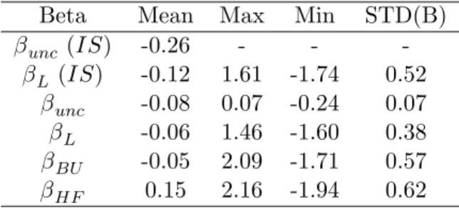
2.1 Descriptive statistics of di¤erent betas of momentum. . . 72

2.2 Performance of time-varying betas in explaining excess

returns and risk of the momentum strategy. . . 72

2.3 Descriptive statistics of the conditional betas for the

Fama-French model. . . 73

2.4 Performance of time-varying betas with respect to the

Fama-French factors in explaining excess returns and risk. 76

2.5 Performance of the hedged portfolios. . . 76

3.1 The long-run performance of momentum compared to the

Fama-French factors. . . 102

3.2 AR (1) of 1-month realized variances. . . 102

3.3 Momentum and the economic gains from scaling. . . 103

3.4 The economic performance of momentum for a

represen-tative investor. . . 103

(6)

List of Figures

1.1 The performance of Deutsche Bank currency ETFs (in

euros). . . 54

1.2 The estimates of the coe¢cients of the portfolio in the

OOS period from 1996:03 to 2011:12. . . 55

1.3 OOS performance of the strategies versus naive portfolios

in the period of 1996:03 to 2011:12. . . 56

1.4 The OOS value of currency strategies for investors

ex-posed to di¤erent background risks. . . 57

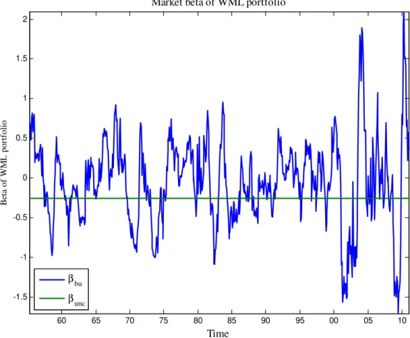
2.1 Bottom-up and unconditional beta of the WML portfolio. 73

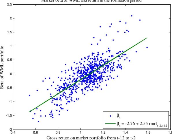
2.2 The bottom-up market beta of the WML portfolio and

the previous return on the market portfolio. . . 74

2.3 The loading of the WML on the FF factors (bottom-up

(7)

3.1 The long-run cumulative returns of momentum compared

to the Fama-French factors. . . 104

3.2 Momentum crashes. . . 105

3.3 The long-run performance of risk-managed momentum. . 106

3.4 The realized volatility of momentum. . . 107

3.5 The density of plain momentum and risk-managed

mo-mentum. . . 108

3.6 The bene…ts of risk-management in the 1930’s and the 00’s.109

(8)

Acknowledgements

The PhD program is a long process. I remember the …rst day of classes

but not as if it were yesterday. Many people helped me along the way

and I’m deeply grateful to them.

First, I am thankful to Pedro Santa-Clara, my supervisor. Besides

being an inspiring professor, I felt encouraged from the onset to follow on

his example and face research work with a bold attitude and an unique

combination of rigor, creativity and critical thinking. I learned a great

deal on how to do research with him, particularly when I had the chance

to become his coauthor, a honour I treasure. In particular, I am grateful

as he went beyond the role of a supervisor to provide crucial support

during some rough patches. He was completely available and always

insightful.

I am grateful to Ana Balcão Reis, who guided me through the taught

part of the program as PhD coordinator. She was always supportive and

(9)

professors of the taught part were always available to help me progress

as a student. I would specially mention Iliyan Georgiev. The learning

experience in his courses is unforgettable. I am also grateful to Paula

Fontoura, the supervisor of my master’s dissertation, who …rst

encour-aged me to do research work.

I am grateful to colleagues: Arash Aloosh, Daniel Monteiro, Luís

Fitchner, José Faias, Rúben Branco and Tymur Gabuniya. Research

work is lonely without someone to share experiences. Specially Arash

and Daniel, doing the group work with them as students in Pedro

Santa-Clara’s course was a great and life changing experience for me. José Faias

comments and advises were precious.

Financial support from FCT (doctoral grant SFRH/BD/42087/2007)

is kindly acknowledged.

Finally, and most of all, I am grateful to my family. My mother Ana

for her example of perseverance in the face of adversity, my father Pedro

for teaching me most of the values I hold dear, my brother Nuno for the

joy he brings to my life and my dear wife Catarina who makes me feel

lucky everyday. I dedicate my dissertation to them and the memory of

(10)

Introduction

My PhD thesis consists of three independent essays: one on extensions

to the carry trade and two on stock momentum. As independent essays

they do not share much in common, but there is an underlying theme:

…nancial market anomalies. In general anomalies are interesting because

they should not exist. As such they are of obvious relevance in any

scienti…c …eld.

In the case of …nancial markets, returns should be a reward for risk.

Otherwise there would be no investors willing to bear those risks. But

some strategies seem to o¤er returns with only elusive relations with

fundamental sources of risk.

For example, the carry trade borrows from low interest rate

curren-cies to invest in high yielding ones. Standard macroeconomics manuals

explain that interest rate di¤erentials should forecast o¤setting

move-ments in currencies. Empirically that is not the case. Hence the returns

(11)

Investment strategies exploiting the information in past returns should

not produce abnormal pro…ts either. That seems to violate weak-form

market e¢ciency. But exploiting past information in returns is exactly

what momentum does.

Of course, what seems anomalous is not necessarily so. The returns

of carry or stock momentum can be rewards for running some

misun-derstood set of risks.

For instance, both the carry trade and stock momentum exhibit large

crash risk. These strategies can be characterized as “picking up pennies

in front of a steamroller”. A recurrent theme in my thesis is whether the

threat of the steamroller explains the persistency of these anomalies.

My …rst essay is on the carry trade. It is a coauthored chapter with

my supervisor, Pedro Santa-Clara. Most research on the carry trade

focuses on that strategy alone, improving the understanding of both its

risk and returns.

The intuition behind our approach is that there is no obvious

rea-son investors in currencies should restrict themselves to carry strategies.

There is pervasive evidence of value and momentum e¤ects across asset

classes and we test its relevance in currency investments. It turns out

that these contribute a lot to portfolio performance.

(12)

other naive benchmarks in out-of-sample tests. Its returns are not

ex-plained by risk and are valuable to diversi…ed investors holding stocks

and bonds. One important result is that crash-risk is a poor

explana-tion for these returns. A currency speculator can combine the carry

with other approaches, obtaining less crash risk. Most notably, a

port-folio combining stocks and bonds with diversi…ed currency investments

hasless crash risk than one without currencies.

The second essay is on the time-varying beta of the momentum

strat-egy. Previous research shows some convincing evidence that the beta of

momentum changes over time. It was puzzling to me why this

previ-ous research did not estimate the betas the most straightforward way:

bottom-up from the betas of individual stocks in the portfolio. I do just

that and …nd the unconditional beta of momentum is highly

mislead-ing. The bottom-up beta of momentum, estimated from the betas of

individual stocks, varies substantially over time. Using bottom-up betas

explains up to 40% of the risk of momentum, out-of-sample. This is

17 times more than one unconditional model achieves and outperforms

other measures of time-varying beta. But like previous research, I …nd

that hedging in real time the time-varying systematic risk of momentum

does not avoid its crashes.

(13)

the …rst essay, this is a coauthored chapter with my supervisor. In a …rst

step we wanted to assess if an investor with reasonable risk aversion …nds

momentum attractive in spite of its rare but intense crashes. We found

the answer to be negative. But then we noticed the crashes of momentum

are not at all like those in the overall stock market. Momentum risk is

quite predictable. The major source of predictability does not come from

systematic risk but from momentum-speci…c risk. Managing this

time-varying risk virtually eliminates crashes and nearly doubles the Sharpe

ratio of the strategy. We argue that momentum per se is not a very

interesting strategy. It provides long runs of attractive returns. But it

has also produced sudden crashes that took 30 years or more to recover

from. By contrast, risk-managed momentum is more of a puzzle.

Overall, the results of my research do not support the steamroller

hypothesis, either for the carry or the stock momentum strategy.

The carry trade crashes. But in a mean-variance world we know risk

is not about variance but rather about covariance. Similarly, in a world

of fat tails and crashes, risk should not be about the crashes per se but

rather about “co-crashes”. As a matter of fact the carry does not crash

simultaneously with value and momentum. Quite the opposite.

In the case of stock momentum, the steamroller does speed up some

(14)

(15)

Chapter 1

Beyond the Carry Trade:

Optimal Currency

Portfolios

0

1.1 Introduction

Currency spot rates are nearly unpredictable out of sample (Meese and

Rogo¤ (1983)).1 Usually, unpredictability is seen as evidence supporting

market e¢ciency, but with currency spot rates it is quite the opposite – it

presents a challenge. Since currencies have di¤erent interest rates, if the

di¤erence in interest rates does not forecast an o¤setting depreciation,

then investors can borrow the low yielding currencies to invest in the high

0_{We thank Andreas Schrimpf, Adrien Verdelhan, Geert Bekaert, Hanno Lustig,}

Harald Hau, Maik Schmeling and Nick Roussanov as well as seminar participants at NOVA, the 2011 QED meeting, the 2012 European Winter Finance Summit in Davos, the 2012 INFER annual meeting, and three anonymous referees for their helpful comments and suggestions. We also thank Craig Burnside and Matti Suominen for letting us use their data.

1_{See also Cheung, Chinn, and Pascual (2005), Rogo¤ and Stavrakeva (2008),}

(16)

yielding ones (Fama (1984)). This strategy, known as the carry trade,

has performed extremely well and for a long period without any sensible

economic explanation. Burnside, Eichenbaum, and Rebelo (2008) show

that a well-diversi…ed carry trade attains a Sharpe ratio that is more

than double that of the US stock market – itself a famous puzzle (Mehra

and Prescott (1985)).

Considerable e¤ort has been devoted to explaining the returns of the

carry trade as compensation for risk. Lustig, Roussanov, and Verdelhan

(2011a) show that the risk of carry trades across currency pairs is not

completely diversi…able, so there is a systematic risk component. They

form an empirically motivated risk factor – the return of high-yielding

currencies minus low-yielding currencies (HM LF X) – close in spirit to

the stock market factors of Fama and French (1992) and show that

it explains the carry premium. But the HM LF X is itself a currency

strategy, so linking its returns to more fundamental risk sources is an

important challenge for research in the currency market.

Some risks of the carry trade are well known. High yielding

cur-rencies are known to “go up by the stairs and down by the elevator,”

implying that the carry trade has substantial crash risk. Carry performs

worse when there are liquidity squeezes (Brunnermeier, Nagel, and

(17)

Sarno, Schmeling, and Schrimpf (2011a)). Its risk exposures are also

time-varying, increasing in times of greater uncertainty (Christiansen,

Ranaldo, and Söderllind (2010)).

Another possible explanation of the carry premium is that there is

some “peso problem” with the carry trade – the negative event that

justi…es its returns may simply have not occurred yet.2 Using options

to hedge away the “peso risk” reduces abnormal returns, lending some

support to this view, but the remaining returns depend crucially on the

option strategy used for hedging (Jurek (2009)).

Despite our improved understanding of the risk of the carry trade,

the fact remains that conventional risk factors from the stock market

(market, value, size, momentum) or consumption growth models, do not

explain its returns.3 Indeed, an investor looking for signi…cant abnormal

returns with respect to, say, the Fama-French factors (1992), would do

very well by just dropping all equities from the portfolio and investing

entirely in a passively managed currency carry portfolio instead.

But there is more to the currency market than just the carry trade.

Market practitioners follow other strategies, including value and

mo-mentum (Levich and Pojarliev (2011)). The bene…ts of combining these

2_{Barro (2006), Fahri and Gabaix (2007), Gourio, Siemer, and Verdelhan (2011),}

Burnside, Eichenbaum, Kleshchelski, and Rebelo (2011).

(18)

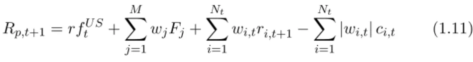
di¤erent approaches became apparent during the height of the …nancial

crisis when events in the currency market assumed historical

propor-tions.4 Figure 1.1 shows the performance of three popular Deutsche

Bank ETFs that track these strategies with the currencies of the G10.

From August 2008 to January 2009, the carry ETF experienced a severe

crash of 32.6%, alongside the stock market, commodities and high yield

bonds. Even so, this crash was not the “peso event” needed to

rational-ize its previous returns.5 But in the same period, the momentum ETF

delivered a 29.4% return and the value ETF a 17.8% return. So while

the carry trade crashed, a diversi…ed currency strategy fared quite well

in this turbulent period.

Coincidently, the literature on alternative currency investments saw

major developments since 2008. Menkho¤, Sarno, Schmeling and Schrimpf

(2011b) document the properties of currency momentum, Burnside (2011)

examines a combination of carry and momentum, Asness, Moskowitz,

and Pederson (2009) study a combination of value and momentum in

currencies (and other asset classes), and Jordà and Taylor (2009)

com-bine carry, momentum and the real exchange rate.

Most of the studies on alternative currency strategies focus on simple,

4_{Melvin and Taylor (2009) provide a vivid narrative of the major events in the}

currency market during the crisis.

(19)

equal-weighted portfolios. The choice of simple portfolios is

understand-able as there is substantial evidence indicating these typically

outper-form out-of-sample more complex optimized portfolios.6 However, we

…nd that using the historical data up to 2007, an investor would have no

reason to want to equal-weight momentum, value and carry. Optimized

portfolios are a closer re‡ection of the uncertainties faced by investors

in real time. Namely, they have to deal with the choice of what signals

to use, how to weigh each signal, and how to address measurement error

and transaction costs.

To study the risk and return of currency strategies in a more realistic

setting, we use the parametric portfolio policies approach of Brandt,

Santa-Clara, and Valkanov (2009) and test the relevance of di¤erent

variables in forming currency portfolios.

First, we use a pre-sample test to study which characteristics

mat-ter for investment purposes. We test the relevance of the inmat-terest rate

spread (and its sign), momentum and three proxies for value: reversal,

the real exchange rate, and the current account. Including all

charac-teristics simultaneously in the test, allows us to see which are relevant

and which are subsumed by others. Then we conduct a comprehensive

out-of-sample (OOS) exercise with 16 years of monthly returns. This

(20)

aims to minimize forward-looking bias – though it does not eliminate it

completely.7

We …nd that the interest rate spread, momentum and reversal

cre-ate economic value for investors whereas fundamentals as the current

account and the real exchange rate don’t. The strategy combining the

relevant signals increases the Sharpe ratio relative to an equal-weighted

carry portfolio from 0.57 to 0.86, out-of-sample and after transaction

costs. This is a 0.29 gain, about the same as the Sharpe ratio of the

stock market in the same period.

Transaction costs matter in currency markets. Taking transaction

costs into account in the optimization further increases the Sharpe ratio

to 1.06, a total gain of 0.49 over the equal-weighted carry benchmark.

The gains in certainty equivalent are even more expressive as the optimal

diversi…ed strategy substantially reduces crash risk.

Unlike the typical result in OOS tests of optimized equity portfolios,

we …nd that the optimized portfolio outperforms all naive benchmarks.8

Also, the risk factors recently proposed to explain carry returns do not

explain the returns of the optimized portfolio, which has monthly ’s

7_{After all, would we be conducting the same out-of-sample exercise in the …rst}

place if there were no indications in the literature that momentum and value worked in recent years? Still, unlike naive portfolios, our strategy will not invest in these signals more than justi…ed by the historical data up to each moment in time.

8_{Brandt, Santa-Clara, and Valkanov (2009) optimized portfolio of stocks also}

(21)

ranging between 1.73 and 2.38 percent. So, while these risk factors may

have some success explaining carry returns, they struggle to make sense

of our optimal currency strategy.

We assess the bene…ts of diversi…cation across currency investment

strategies for investors already exposed to other asset classes. We …nd

an average increase in the Sharpe ratio of 0.51, a much more impressive

gain than the one documented in Kroencke, Schindler, and Schrimpf

(2011). Furthermore, including the currency strategies in the portfolio

consistently reduces fat tails and left skewness. This contradicts

crash-risk explanations for returns in the currency market.

Finally, we regress the returns of the optimal strategy on the level of

speculative capital in the market, following Jylhä and Suominen (2011).

We …nd evidence that the returns of the strategy decline as the amount

of hedge fund capital increases. This suggests that the returns we

docu-ment constitute an anomaly that is gradually being arbitraged away by

hedge funds.

This chapter is structured as follows. In section 1.2 we explain

the implementation of parametric portfolios of currencies. Section 1.3

presents the empirical analysis. Section 1.3.1 describes the data and the

variables used in the optimization. Sections 1.3.2 and 1.3.3 present the

(22)

respectively. Section 1.4 compares the performance of the optimal

port-folio with naive benchmarks. In Section 1.5 we test the risk exposures

of the optimal portfolio. In Section 1.6 we assess the value of currency

strategies for investors holding stocks and bonds. Section 1.7 discusses

possible explanations for the abnormal returns of the strategy, including

insu¢cient speculative capital early in the sample.

1.2 Optimal parametric portfolios of currencies

We optimize currency portfolios from the perspective of an US investor

in the forward exchange market. In the forward exchange market,

the investor can agree at time t to buy currency i at time t+ 1 for

1=Fi

t;t+1 where Ft;ti +1 is the price of one USD expressed in foreign cur-rency units (FCU). Then at timet+1the investor liquidates the position selling the currency for1/Si

t+1; whereSti+1 is the spot price of one USD in FCU. The return (in US dollars) of a long position in currencyi in monthtis:

ri_t₊₁ = F i t;t+1 Si

t+1

1 (1.1)

This is a zero-investment strategy as it consists of positions in the

forward market only.9 We use one-month forwards throughout as is

(23)

standard in the literature.10 _{Therefore all returns are monthly and there}

are no inherited positions from month to month. This also avoids

path-dependency when we include transaction costs in the analysis.

We optimize the currency strategies using the parametric portfolio

policies approach of Brandt, Santa-Clara, and Valkanov (2009). This

method models the weights of assets as a function of their characteristics.

The implicit assumption is that the characteristics convey all relevant

information about the assets’ conditional distribution of returns. The

weight on currencyiat time tis:

wi;t = Txi;t=Nt (1.2)

where xi;t is a k 1 vector of currency characteristics, is a k 1 parameter vector to be estimated and Nt is the number of

curren-cies available in the dataset at time t. Dividing by Nt keeps the policy

stationary (see Brandt, Santa-Clara, and Valkanov (2009)). We do not

place any restriction on the weights, which can be positive or negative.

This re‡ects the fact that in the forward exchange market there is no

obvious non-negativity constraint.

The strategies we examine consist of an investment of 100% in the

We ignore that in this study.

1 0_{Burnside, Eichenbaum, and Rebelo (2008), Burnside (2011), Burnside,}

(24)

US risk-free asset, yielding rfU S

t ;and a long-short portfolio in the

for-ward exchange market. For a given sample, uniquely determines a

parametric portfolio policy, and the corresponding return each period

will be:

rp;t+1 =rftU S+ Nt X

i=1

wi;trti+1 (1.3)

The problem an investor faces is optimizing its objective function

picking the best possible for the sample:

maxEt[U(rp;t+1)] (1.4)

We use power utility as the objective function:

U(rp) =

(1 +rp)1

1 (1.5)

where is the coe¢cient of relative risk aversion (CRRA).11 The main

advantage of this utility function is that it penalizes kurtosis and

skew-ness, as opposed to mean-variance utility, which focuses only on the …rst

two moments of the distribution of returns. So our investor dislikes crash

risk and values characteristics that help reduce it, even if these do not

1 1_{Bliss and Panigirtzoglou (2004) estimate} _{empirically from risk-aversion implicit}

(25)

add to the Sharpe ratio.

The main restriction imposed on the investor’s problem is that is

kept constant across time. This substantially reduces the chances for

in-sample over…tting as only ak 1 vector of characteristics is estimated. The assumption that does not change allows its estimation using the

sample counterparts:

^ = arg max 1

T

T_X1

t=0

U rf_tU S+ Nt X

i=1

( Txi;t=Nt)rit+1

!

(1.6)

For statistical inference purposes, Brandt, Santa-Clara, and Valkanov

(2009) show that we can use either the asymptotic covariance matrix of

^_{or bootstrap methods.}12

For the interpretation of results it is important to note that (1.6)

optimizes a utility function and not a measure of the distance between

forecasted and realized returns. Therefore, can be found relevant for

one characteristic even if it conveys no information at all about expected

returns. The characteristic may just be a predictor of a currency’s

con-tribution to the overall skewness or kurtosis of the portfolio, for example.

Conversely, a characteristic may be found irrelevant for investment

pur-poses even if it does help in forecasting returns. Indeed, it may forecast

1 2_{We use bootstrap methods for standard errors in the empirical part of this paper,}

(26)

both higher returns and higher risk for a currency, o¤ering a trade-o¤

that is irrelevant for the investor’s utility function.

Menkho¤, Sarno, Schmeling, and Schrimpf (2011b) show that

mo-mentum strategies incur higher transaction costs than the carry trade.

They even …nd that momentum pro…ts are of little relevance in

curren-cies of developed countries after transaction costs. So one valid concern

is whether the gains of combining momentum with carry persist after

taking into consideration time and cross-currency variation in

transac-tion costs. Fortunately, parametric portfolio policies can easily

incorpo-rate transaction costs that vary across currencies and over time. This is

a particularly appealing feature of the method, since transaction costs

varied substantially as foreign exchange trading shifted towards

elec-tronic crossing networks.

To address this issue we optimize:

^ = arg max 1

T

T_X1

t=0

U rf_tU S+ Nt X

i=1

( Txi;t=Nt)rti+1

Nt X

i=1

T_x

i;t=Nt ci;t

!

(1.7)

where ci;t is the transaction cost of currency i at time t; which we

cal-culate as:

ci;t =

F_t;task₊₁ F_t;tbid₊₁ Fask

t;t+1+Ft;tbid+1

(1.8)

(27)

This assumes the investor buys (sells) a currency in the forward market

at the ask (bid) price, and the forward is settled at the next month’s

spot rate. This may overstate transaction costs. For instance, Mancini,

Ranaldo, and Wrampelmeyer (2011) document that e¤ective costs in the

spot market are less than half those implied by bid-ask quotes as there

is signi…cant within-quote trading.

There is another important point to highlight about transaction

costs: for a given month and currency, these are proportional to the

absolute weight put on that particular currency. This absolute weight is

a function of all the currency characteristics as seen in equation 1.2, so

transaction costs will depend crucially on the time-varying interaction

between characteristics. One example is the interaction between

momen-tum and other characteristics. As Grundy and Martin (2001) show for

stocks, the way momentum portfolios are built guarantees time-varying

interaction with other stock characteristics. For instance, after a bear

market, winners tend to be low-beta stocks and the reverse for losers. So

the momentum portfolio, long in previous winners and short in previous

losers, will have a negative beta. The opposite holds after a bull market.

The same applies for currencies, after a period where carry experienced

high returns, high yielding currencies tend to have positive momentum.

(28)

absolute weights and thus higher transaction costs. However, after

neg-ative carry returns the opposite happens: high yielding currencies have

negative momentum. So momentum partially o¤sets the carry signal

resulting in smaller absolute weights and actually reduces the overall

transaction costs of the portfolio. This means the transaction costs of

including momentum for an extended period of time in a diversi…ed

portfolio policy will be lower than what one …nds examining momentum

in isolation as in Menkho¤, Sarno, Schmeling, and Schrimpf (2011b).

1.3 Empirical analysis

As …gure 1.1 shows, combining reversal and momentum with the carry

trade considerably mitigated the crash of the carry trade in the last

quarter of 2008. Yet this is easy to point out ex post. The relevant

question is whether investors in the currency market had reasons to

believe in the virtue of diversifying their investment strategy before the

2008 crash. For example, Levich and Pojarliev (2011) examine a sample

of currency managers and …nd that they explored carry, momentum

and value strategies before the crisis but shifted substantially across

investment styles over time. In particular, right before the height of

the …nancial crisis in the last quarter of 2008, most currency managers

(29)

investingagainst value. This raises the question of whether the bene…ts

of diversi…cation were as clear before the crisis as they later became

apparent. Equally weighting carry, momentum, and value was not an

obvious strategy at the time. This also shows that what appear to be

naively simple strategies such as equal weighting carry, momentum, and

value are not naive at all and in fact bene…t a lot from hindsight.

To address this issue we conduct two tests: i) a pre-sample test with

the …rst 20 years of data up to 1996 to determine which characteristics

were relevant back then; ii) an out-of-sample experiment since 1996 in

which the investor chooses the weight to put on each signal using only

historical information available up to each moment in time.

Section 1.3.1. explains the data sources and the variables used in our

optimization. In section 1.3.2. we conduct the pre-sample test with the

sample from 1976:02 to 1996:02. In section 1.3.3. we conduct the

out-of-sample experiment of portfolio optimization using only the relevant

variables identi…ed in the pre-sample test.

1.3.1 Data

We use data on exchange rates, the forward discount / premium, and

the real exchange rate for the Euro zone and 27 member countries of the

Organization for Cooperation and Development (OECD). The countries

(30)

Re-public, Denmark, Finland, France, Germany, Greece, Hungary, Ireland,

Italy, Japan, Mexico, Netherlands, New Zealand, Norway, Poland,

Por-tugal, Slovakia, South Korea, Spain, Sweden, Switzerland, the UK, and

the US.

The exchange rate data are from Datastream. They include spot

exchange rates at monthly frequency from November 1960 to December

2011 and one-month forward exchange rates from February 1976. As in

Burnside, Eichenbaum, Kleshchelski, and Rebelo (2011) we merge two

datasets of forward exchange rates (against the USD and the GBP) to

have a comprehensive sample of returns in the forward market in the

‡oating exchange rate era.13

We calculate the real exchange rates of each currency against the

USD using the spot exchange rates and the consumer price index. The

Consumer Price Index (CPI) data come from the OECD/Main Economic

Indicators (MEI) online database. For the Euro, the series that starts

January 1996 was extended back to January 1988 using the weights of

the Euro founding members. In the case of Australia, New Zealand, and

Ireland (before November 1975) only quarterly data are available. In

those cases, the value of the last available period was carried forward to

1 3_{The …rst dataset has data on forward exchange rates (bid and ask quotes) against}

(31)

the next month.

We test the economic relevance of carry, momentum, and value

prox-ies combined in a currency market investment strategy. The variables

used in the optimization exercise are:

1. sign_i;t: The sign of the forward discount of a currency with respect

to the USD. It is 1 if the foreign currency is trading at a discount

(Fi;t> Si;t)and -1 if it trades at a premium. This is the carry trade

strategy examined in Burnside, Eichenbaum, and Rebelo (2008),

Burnside (2011), Burnside, Eichenbaum, Kleshchelski, and Rebelo

(2011). Given the extensive study of this strategy we adopt it as

the benchmark throughout the analysis.

2. fdi;t: The interest rate spread or the forward discount on the

cur-rency. We standardize the forward discount using the cross-section

mean and standard deviation across all countries available at time

t, _{F D}_t and F Dt respectively. Speci…cally, denoting the

(unstan-dardized) forward discount as F Di;t; we obtain the standardized

discount as: f di;t =

F Di;t _{F Dt}

F Dt : This cross-sectional

standardiza-tion measures the forward discount in standard deviastandardiza-tions above or

below the average across all countries. By construction, a variable

standardized in the cross-section will have zero mean, implying

(32)

dollar). Jurek (2009) shows that an interest rate spread strategy

similar to this outperforms the equally-weighted carry trade based

on sign.

3. momi;t: For currency momentum we use the cumulative currency

appreciation in the last three-month period, cross-sectionally

stan-dardized. This variable explores the short-term persistence in

cur-rency returns. We use momentum in the previous three months

because there is ample evidence for persistence in returns for

port-folios with this formation period while there are no signi…cant gains

(in fact the momentum e¤ect is often smaller) considering longer

formation periods (see Menkho¤, Sarno, Schmeling, and Schrimpf

(2011b)). Three-month momentum was also used in Kroencke,

Schindler, and Schrimpf (2011). Cross-sectional standardizations

means that momentum measures relative performance. Even if all

currencies fall relative to the USD those that fall less will have

positive momentum.

4. revi;t: Long-term reversal is the cumulative real currency

depre-ciation in the previous …ve years, standardized cross-sectionally.

First we calculate the cumulative real depreciation of currency

(33)

num-ber Qi;h;t =

Si;tCP Ii;h 2CP ItU S2

Si;hCP Ii;t 2CP IU Sh 2

:We use a two-month lag to ensure the CPI is known. We pick h = t 60 which corresponds to 5 years:Then we standardizeQi;h;t cross-sectionally to obtainrevi;t:

This is essentially the same as the notion of “currency value” used

in Asness, Moskowitz, and Pederson (2009). We just use the

cu-mulative deviation from purchasing power parity, instead of the

cumulative return as they did, to obtain a longer out-of-sample

test period. Reversal is positive for those currencies that

experi-enced the larger real depreciations against the USD in the previous

5 years and negative for the others.

5. qi;t: The real exchange rate standardized by its historical mean

and standard deviation. First, as for reversal, we computeQi;hi;twith

the di¤erence that here the basis period (hi)is the …rst month for

which there is CPI and exchange rate data available for currency

i. Then we compute qi;t =

Q_i;hi;t Qi;t

Qi;t ; where Qi;t is the historical

average Pt

j=hi

Qi;hi;j=tand Qi;t is the historical standard deviation

fQi;hi;jg

t

j=hi :The real exchange rate is measured in standard

deviations above or below the historical average. Jordà and Taylor

(2009) also used the demeaned real exchange rate but our time

se-ries standardization ensures only information available up to each

(34)

standardized,q is not neutral in terms of the basis currency (the USD). It will tend to be positive for all currencies when these are

undervalued against the USD by historical standards.

6. cai;t: The current account of the foreign economy as a percentage

of Gross Domestic Product (GDP), standardized cross-sectionally.

The optimization assumes that the previous year current account

information becomes known in April of the current year. The

cur-rent account data were retrieved from the Annual Macroeconomic

database of the European Commission (AMECO), where data are

available on a yearly frequency from 1960 onward. Many studies

examine the relation between the current account and exchange

rates justifying its inclusion as a conditional variable.14

In order to be considered for the trading strategies, a currency must

satisfy three criteria: i) there must be ten previous years of real

ex-change rate data; ii) current forward and spot exex-change quotes must be

available; and iii) the country must be an OECD member in the period

considered. After …ltering out missing observations, there are a

mini-mum of 13 and a maximini-mum of 21 currencies in the sample. On average

there are 16 currencies in the sample.

1 4_{See, for example, Dornbusch and Fischer (1980), Obstfeld and Rogo¤ (2005),}

(35)

1.3.2 Pre-sample results

Table 1.1 shows the investment performance of the optimized strategies

from 1976:02 to 1996:02. We use this pre-sample period to check which

variables had strong enough evidence supporting their relevance back in

1996, before starting the out-of-sample experiment.

The two versions of the carry trade (sign and f d) deliver similar performance, with high Sharpe ratios (0.96 and 0.99, respectively) but

also with signi…cant crash risk (as captured by excess kurtosis and

left-skewness). Momentum provides a Sharpe ratio of 0.56, better than

the performance of the stock market of 0.40 in the same sample. This

con…rms the results of Okunev and White (2003), Burnside,

Eichen-baum and Rebelo (2011), and Menkho¤, Sarno, Schmeling, and Schrimpf

(2011b).

Financial predictors work better in our optimization than

fundamen-tals like the real exchange rate and the current account. Reversal had an

interesting Sharpe ratio of 0.36. This con…rms the results of Menkho¤,

Sarno, Schmeling, and Schrimpf (2011b) and Asness, Moskowitz, and

Pederson (2009). The strategies using the current account and the real

exchange rate as conditioning variables achieved modest Sharpe ratios

(36)

in-sample optimization.15

The seventh row shows the performance of an optimal strategy

com-bining the carry (both sign and f d) with momentum and reversal – all the statistically relevant variables. Already in 1996 there was ample

evidence indicating that a strategy combining di¤erent variables lead to

substantial gains. The Sharpe ratio of the optimal strategy was nearly

40% higher than the benchmark and it produced a 16.43 percentage

points gain in annual certainty equivalent.

Adding fundamentals to this strategy does not improve it: the Sharpe

ratio increases only 0.01 and the annual certainty equivalent only 13

ba-sis points. An insigni…cant gain since in-sample any additional variable

must always increase utility.

Table 1.2 shows the statistical signi…cance of the variables, isolated

and in combination. The table presents the point-estimates of the

co-e¢cients and the bootstrapped p-values (in brackets). We perform the

bootstrap by generating 1,000 random samples drawn with replacement

from the original sample and with the same number of observations (240

months of returns and respective conditional variables). Then we …nd

the optimal coe¢cients in each random sample, thereby obtaining their

1 5_{We also tested these variables out-of-sample (although, based on the in-sample}

(37)

distribution across samples.

Taken in isolation, the carry trade variables (sign and f d) and mo-mentum are all signi…cant at the 1% level. Reversal has a p-value of

5.3%.

The current account and the real exchange rate have the wrong sign

(underweighting undervalued currencies and those with strong current

accounts) but are not signi…cant. We have known since Meese and Rogo¤

(1983), currency spot rates are nearly unpredictable by fundamentals.

Using time-series methods, Gourinchas and Rey (2007) …nd that the

current account forecasts the spot exchange rate of the US dollar against

a basket of currencies.16 But we …nd no evidence in the cross section

that the current account is relevant for designing a pro…table portfolio

of currencies. At best, the fundamental information is subsumed by

interest rates, momentum and reversal.

Combining all variables con…rms our main result. Carry, momentum

and reversal are relevant for the optimization, fundamentals are not.

The …nal row shows the results for an optimization using only the

vari-ables deemed relevant. The p-values show the four varivari-ables contribute

signi…cantly to the economic value of the strategy in combination.

Concerning both carry variables (sign and f d), the correlation of

1 6_{Gourinchas and Rey (2007) derive their result making a di¤erent use of the current}

(38)

their returns was 0.46 from 1976:02 to 1996:02, a value that has not

changed much since. So these two ways of implementing the carry trade

are not identical and the investor …nds it optimal to use both. The

signvariable assigns the same weight to a currency yielding 0.1% more than the USD as to another yielding 5% more. In contrast, the f d variable assigns weights proportionally to the magnitude of the interest

rate di¤erential. Whenever the USD interest rate is close to the extremes

of cross section, thesignis very exposed to variations in its value, while f dis always dollar-neutral.

One word of caution on forward-looking bias is needed here. Our

in-sample test shows that in 1996 some of the strategies recently

pro-posed in the literature on currency returns would already be found to

have an interesting performance. This is a necessary condition to assess

if investors would want to use these variables in real time to build

diver-si…ed currency portfolios. However, this does not tell us whether there

were other investment approaches that would have seemed relevant in

1996 and resulted afterwards in poor economic performance.

1.3.3 Out-of-sample results

We perform an out-of-sample (OOS) experiment to test the robustness of

the optimal portfolio combining carry, momentum, and value strategies.

(39)

months of the sample. Then the model is re-estimated every month,

using an expanding window of data, until the end of the sample. The

out-of-sample returns thus obtained minimize the problem of look-ahead

bias. We do not useq and cain the optimization as these failed to pass the in-sample test with data until 1996.17

The in-sample results also hold out of sample. Table 1.3 shows that

the model using interest rate variables, momentum and reversal achieves

a certainty equivalent gain of 10.84 percent over the benchmark, with

better kurtosis and skewness. Its Sharpe ratio is 1.15, a gain of 0.45 over

the benchmarksignportfolio.

Transaction costs can considerably hamper the performance of an

investment strategy. For example, Jegadeesh and Titman (1993)

pro-vide compelling epro-vidence that there is momentum in stock prices, but

Lesmond et al. (2004) …nd that after taking transaction costs into

con-sideration there are little to no gains to be obtained in exploiting

mo-mentum.

Panel B of table 1.3 shows the OOS performance of the strategies

after taking transaction costs into consideration. Clearly transaction

costs matter. The Sharpe ratio of the optimal strategy is reduced by

0.29, a magnitude similar to the equity premium, and the certainty

1 7_{Although including these does not change much the results as they receive little}

(40)

equivalent drops from 18.87 percent to just 12.15 percent. Momentum

and reversal individually show no pro…tability at all after transaction

costs. This …nding mirrors the results of Lesmond et al. (2004) with

regard to stock momentum. It also con…rms the result in Menkho¤,

Sarno, Schmeling, and Schrimpf (2011b) that there are no signi…cant

momentum pro…ts in currencies of developed countries after transaction

costs.

But we …nd that transaction costs can be managed. In panel C

we adjust the optimization to currency and time-speci…c transaction

costs. We calculate the cost-adjusted interest rate spread variable as:

g

F Di;t=sign(F Dit)(jF Ditj cit) and standardize it in the cross-section

to getf df_it. We then model the parametric weight function as:

wi;t =I(cit <jF Ditj) Txi;t=Nt (1.9)

whereI(:) is the indicator function, with a value of one if the condition holds and zero otherwise. We maximize expected utility with this new

portfolio policy, estimating after consideration of transaction costs.

This method e¤ectively eliminates from the sample currencies with

prohibitive transaction costs and reduces the exposure to those that

have a high ratio of cost to forward discount. Other, more complex,

(41)

simple approach is enough to prove the point that managing transaction

costs adds considerable value.

The procedure increases the Sharpe ratio of the diversi…ed strategy

from 0.86 to 1.06 and produces a gain in the certainty equivalent of

4.54 percent per year. This gain alone is higher than the momentum

or reversal certainty equivalents per se. Indeed, the performance of the

diversi…ed strategy with managed transaction costs is very close to the

strategy in panel A without transaction costs.

Managing transaction costs is particularly important as these

cur-rency strategies are leveraged. Given the high Sharpe ratios attainable

by investing in currencies, the optimization picks high levels of

lever-age. We de…ne leverage as Lt = Nt P

i=1

jwitj: This is the absolute value

of US dollars risked in the currency strategy per dollar invested in the

risk-free asset. The optimal strategy has a mean leverage of 5.94 in the

OOS period of 1996:03 to 2011:12. As a result, a small di¤erence in

transaction costs can have a large impact in the economic performance

of the strategy.

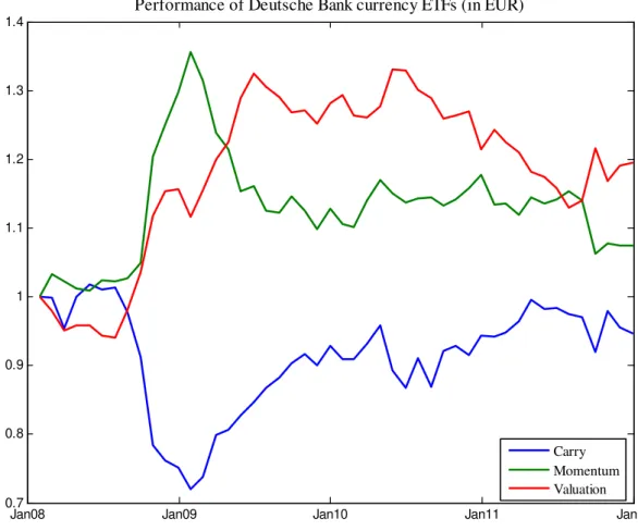
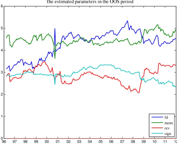
One concern in optimized portfolios is whether in-sample over…tting

leads to unstable and erratic coe¢cients OOS. Figure 1.2 shows the

estimated coe¢cients of the diversi…ed portfolio with managed costs in

(42)

stable, leading to consistent exposure to the conditioning variables.

The optimal diversi…ed portfolio has a robust OOS economic

per-formance. In the next section we compare it with simple strategies

proposed in the literature.

1.4 Comparison with naive currency strategies

We want to assess the importance of using our optimization procedure

by comparing our strategy with simple alternatives. This is especially

important because DeMiguel, Garlappi, and Uppal (2009) show that

simple rules of investment have robust out-of-sample performance when

compared to optimized portfolios. One could argue though that simple

currency strategies are not so naive. The performance of long-short

portfolios depends on the characteristic used to sort currencies in the …rst

place. The choice of characteristics to average is thus crucial. Why carry,

momentum and reversal and not something else? There is the choice of

designing a strategy that is neutral in terms of the basis currency (as

f d) or not (as sign):The weighing of di¤erent currency characteristics is also arbitrary in a naive strategy. So the scope for arbitrary choices

in‡uenced by ex post observation of the data is not necessarily small

for naive strategies. Still, the simple strategies found in the literature

(43)

We compare the economic performance of the optimal diversi…ed

strategy with 5 simple portfolios: i) the sign strategy, which is long currencies yielding more than the USD and short the others; ii) the

version of momentum (momb) proposed in Burnside, Eichenbaum, and

Rebelo (2011) which is long currencies with a positive return in the

previous month and short the others; iii) an equal-weighted combination

of sign and momentum; iv) the interest rate spread strategy (f d); v) an

equal-weighted portfolio of the signals used in our portfolio policy –

momentum, reversal,signand f d.

It is questionable whether the EW strategy is a naive approach since

this strategy uses the signals selected by the optimized portfolio. But

including this EW portfolio allows an assessment of how relevant it is to

manage transaction costs and to allow the coe¢cients in the strategy to

di¤er from equality.

Table 1.4 shows the economic performance of the optimal strategy

compared to the simple alternatives. All strategies include a 100%

in-vestment in the risk free asset complemented with a long-short

cur-rency portfolio. We scale all simple strategies to have constant leverage

throughout the period, set to match the mean leverage of the optimized

strategy. This ensures that di¤erences in performance do not depend on

(44)

opti-mally chosen indirectly in the maximization of the utility function. The

leverage (Lt = Nt P

i=1

jwitj=

Nt P

i=1

j xitj=Nt) depends both on the estimated

coe¢cients and on the level of the explanatory variables and therefore

changes through time. We also include a version of the optimal strategy

with constant leverage to assess if time-varying leverage is important to

performance.

The optimal strategy, with a Sharpe ratio of 1.06 and a certainty

equivalent of 16.69 percent, outperforms all others. The 0.22 gain in

Sharpe ratio with respect to the EW strategy (the ‘naive’ approach

that performed the best) is statistically signi…cant with a p-value of

0.027.18This is because the optimal coe¢cients are not equal (as seen in

Figure 1.2) and the simple strategy does not manage transaction costs.

The gain in certainty equivalent of 7.13 percentage points is even more

expressive.

Perhaps surprising is the unimpressive performance of the

combi-nation of sign and momb: It achieves a lower Sharpe ratio than the

signstrategy alone. This is because leverage is set to a constant level, so the outperformance of this strategy documented in Burnside,

Eichen-baum, and Rebelo (2011) comes from time-varying leverage. Whenever

a currency yields more than the USD but experiences a negative return

(45)

in the previous month, the two signals cancel out resulting in a weight of

zero for the currency. As a result, the combination ofsignandmombhas

time-varying leverage, increasing after months when carry has positive

returns and decreasing otherwise.

The optimal strategy with constant leverage has a good performance,

with a Sharpe ratio of 0.99, though not as good as the unconstrained

strategy. Allowing leverage to change over time leads to lower kurtosis

and less negative skewness.

All in all, the evidence on economic performance is clear: the optimal

strategy produces a certainty equivalent gain of 7.13 percentage points

per year over the best performing naive strategy. This gain is due to a

higher Sharpe ratio and lower crash risk (as captured by kurtosis and

left-skewness).

In table 1.5 we regress the excess returns of the optimal strategy on

those of the simple portfolios to assess its abnormal returns, captured by

the intercept. The t-statistics and R-squares are obviously signi…cant,

since the optimal strategy is built with similar variables as the naive

strategies. But these variables do not fully explain the excess returns

which range from 0.68 to 2.28 percent per month. The optimal strategy

shows an abnormal return of 8.16 percent per year with respect to the

(46)

Figure 1.3 shows the cumulative excess returns of each naive strategy

compared to the optimal diversi…ed portfolio. We also include the excess

return on the stock market portfolio for comparison. Currency strategies

in general outperform the stock market. The Sharpe ratio of the stock

market in the OOS period is 0.29, lower than any currency strategy

examined.

But the graph also shows that no simple portfolio systematically

outperforms the optimal strategy. This contrasts with the result of

DeMiguel, Garlappi, and Uppal (2009) for stocks. This result extends

and con…rms recent …ndings that optimization methods can

outper-form more naive approaches in currency markets (Corte, Sarno, Tsiakas

(2009), Berge, Jordà, and Taylor ( 2010)).

1.5 Risk exposures

Cochrane (2011) uses the expression “factor zoo” to describe the growing

number of risk factors proposed in the literature to explain asset returns.

The literature on currency markets is no exception and many sets of risk

factors have been proposed, mostly to explain the returns of the carry

trade.

Lustig, Roussanov, and Verdelhan (2011a) propose an

(47)

(HM LF X) to explain carry trade returns. This is an approach similar

in spirit to the Fama and French (1992) three-factor model for stock

returns. Note however that the HM LF X factor is itself by

construc-tion a carry portfolio. So while this approach establishes that there

is systematic risk in the carry trade, it does not provide intuition on

what is the fundamental risk source that justi…es its returns.

Brunner-meier, Nagel, and Pederson (2008) argue that liquidity-risk spirals are

the source of risk of the carry trade. They use the innovation in the

TED spread and in the VIX as factors proxying for liquidity and risk.

Menkho¤, Sarno, Schmeling, and Schrimpf (2011a) propose innovations

in foreign exchange market volatility as a risk factor to explain the carry

trade and currency momentum. They also use the innovation in

aver-age transaction costs and argue the information in this is subsumed by

FX volatility. Lustig and Verdelhan (2007) and Lustig, Roussanov, and

Verdelhan (2011b) propose consumption growth risk as a factor to

ex-plain the carry returns. Table 1.6 shows the exposure of the optimal

diversi…ed strategy (with managed transaction costs) to 8 sets of risk

factors.

The …rst model shows that the currency strategy is not exposed to

consumption growth risk.19 This con…rms the results of Burnside (2011)

1 9_{For this we use the monthly growth rate of Real Personal Consumption}

(48)

and Jordà and Taylor (2011).

The second and third models show that our strategy is exposed to

liq-uidity risk (as captured by innovations in the TED spread) and increases

in stock volatility (as captured by the changes in VIX). The VIX is a

more signi…cant variable, its beta has a t-statistic of -3.98 versus -2.90

for the TED spread.

The fourth model regresses the returns of the optimal strategy on

innovations in transaction costs (the cross-section average in the forward

exchange market). This does not yield signi…cant results as the adjusted

R-squared is negative.

The …fth model shows the diversi…ed portfolio, with a t-statistic of

-2.15, is exposed to innovations in foreign exchange volatility con…rming

Menkho¤, Sarno, Schmeling, and Schrimpf (2011a).20 But the adjusted

R-squared is only 1.88, much less than the 7.27 of the VIX.

Our optimal strategy is also somewhat exposed to stock market risk

as the CAPM and the Carhart (1997) models show. But the only

rel-evant variable is the excess return on the market portfolio with a

t-statistic of 4.02 in the CAPM and 4.08 in the Carhart four-factor model.

The best performing model, in term of adjusted R-squared, is the

2 0_{We follow Menkho¤, Sarno, Schmeling, and Schrimpf (2011a) in computing FX}

volatility in montht as: F X;t=D1t

Dt

P

=1 N

P

i=1

jri; j

N ; whereDtis the number of trading

(49)

empirically-motivatedHM LF X factor of Lustig, Roussanov, and

Verdel-han (2011a). In this model we regress the optimal portfolio excess

returns on RX (the dollar-return of an equal-weighted average of all currency portfolios) andHM LF X;the di¤erence in return between the

highest yielding currencies and the lowest yielding currencies.21 The

beta with respect to theHM LF X is clearly signi…cant, with a t-stat of

6.54, and the adjusted R-squared of 20.85 is by far the highest among

the eight models used.

But the most striking result is the consistently high of the

opti-mal strategy, ranging between 1.73 and 2.38 percent per month, always

signi…cant at conventional levels of con…dence. So, while the optimal

strategy is exposed to some of the factors proposed in the literature

on currency returns, the R-squared is typically low and the abnormal

returns highly signi…cant.

There is evidence of time-varying risk exposures in the carry trade

(Christiansen, Ranaldo, and Söderllind (2010)). In particular, the

expo-sure of the carry to the stock market rises after shocks to liquidity and

risk. This is not captured by the unconditional analysis in table 1.6. So

it is of interest to ask whether the optimal strategy also has time-varying

risk.

2 1_{We retrieve the data from Adrien Verdelhan’s webpage. The data is for returns}

(50)

Following Christiansen, Ranaldo, and Söderllind (2010) we run the

following OLS regression:

rp;t rft= + 0RM RFt+ 1RM RFtzt 1+ 2Rbonds ;t+ 3Rbonds ;tzt 1+"t

(1.10)

wherezt 1is a proxy for (lagged) risk andRbonds ;tis the excess return of

the 10 year US bond over the risk-free rate.22 _{As proxies for risk we use}

the foreign exchange volatility, the TED spread, VIX, the average

trans-action cost, and leverage. The …rst four are also used in Christiansen,

Ranaldo, and Söderllind (2010). We add leverage as this is time varying

in the optimal strategy and could naturally induce time-varying risk.

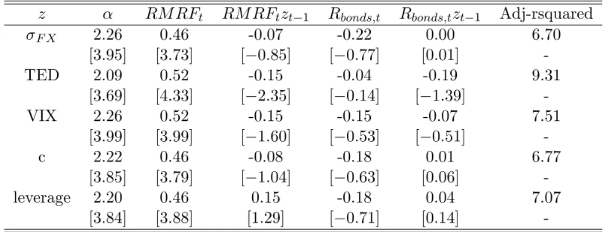
The results of the regression are in table 1.7. The only interaction

term that is signi…cant is for the TED spread with the market. But the

sign of the coe¢cient is negative, implying the strategy is less exposed

to the stock market after a liquidity squeeze. In order for time-varying

risk to explain the returns of the diversi…ed strategy, the opposite should

happen. All other interaction terms are not signi…cant, so time-varying

risk is of little relevance to explain the performance of the diversi…ed

strategy. In particular, there is no evidence that the optimal strategy is

riskier when it is more leveraged. In general, the conditional models do

not add much to the CAPM, and the large signi…cant persists after

(51)

considering time-varying risk.

Either unconditionally or conditionally the risk factors proposed to

explain the carry trade can do very little to explain the returns of our

optimal diversi…ed currency strategy. This indicates that the optimal

strategy exploits market ine¢ciencies rather than loading on factor risk

premiums.

1.6 Value to diversi…ed investors

We assess whether the currency strategies are relevant for investors

al-ready exposed to the major asset classes. Indeed, there is no reason a

priori that investors should restrict themselves to pure currency

strate-gies, particularly when there are other risk factors that have consistently

o¤ered signi…cant premiums as well.

The value of currency strategies to diversi…ed investors holding bonds

and stocks is a relatively unexplored topic. Most of the literature on

the currency market has focused on currency-speci…c strategies. One

exception is Kroencke, Schindler, and Schrimpf (2011) who …nd that

combining investments in stocks and bonds with currencies improves

the Sharpe ratio from 0.34 to 0.43 without entailing an increase in crash

risk.

(52)

constant relative risk aversion of 4. The returns on wealth are now:

Rp;t+1 =rftU S+ M

X

j=1

wjFj+ Nt X

i=1

wi;tri;t+1

Nt X

i=1

jwi;tjci;t (1.11)

where wj are the (constant) weights on a set of M investable factors

F expressed as excess returns, and wi;t depends on the characteristics

and the coe¢cients that maximize utility jointly withwj.

Table 1.8 shows the OOS performance of the portfolios with and

without the currency strategy. The currency strategy combines the

in-terest rate spread, sign, momentum, and long-term reversal.

Subse-quently, each two rows compare a portfolio of investable factors with a

portfolio combining these factors with the currency strategy.

The opportunity to invest in currencies is clearly valuable to

in-vestors. Including currencies in the portfolio always adds to the Sharpe

ratio and raises the certainty equivalent. The OOS gains in certainty

equivalent range between 9.99 percentage points for an investment in

stocks and bonds and 38.04 percentage points for a diversi…ed

invest-ment using the Carhart factors. The gain with respect to the Carhart

factors comes mainly from the dismal performance of stock momentum

in 2009, when it experienced one of its worst crashes in history (Daniel

(53)

These gains are far more impressive than the gains from adding

fac-tors like HML and SMB to the stock market. Indeed, only the inclusion

of bonds improves upon the certainty equivalent of the stock market

OOS. Generally, the inclusion of SMB, HML, and WML factors

im-proves Sharpe ratios, but this increase is o¤set by higher drawdowns,

resulting in lower certainty equivalents.

Including currencies however leads to substantial gains. This extends

the evidence in Burnside (2011) that there is no known set of risk factors

that prices currency and stock returns simultaneously. The relevance of

the interest rate spread, currency momentum, and long-term reversal

to forecast currency returns makes all conventional risk premiums seem

small in comparison.

Including currencies in the portfolio of stocks and bonds produces

increases in the Sharpe ratio as high as 0.81 for a portfolio of US stocks

and currencies. On average adding currency strategies increases the

Sharpe ratio by 0.51. This con…rms the results of Kroencke, Schindler,

and Schrimpf (2011).

One possible justi…cation for the higher Sharpe ratios obtainable by

investing in currencies is that these might entail a higher crash risk –

as Brunnermeier, Nagel, and Pedersen (2008) shows for the carry trade.

(54)

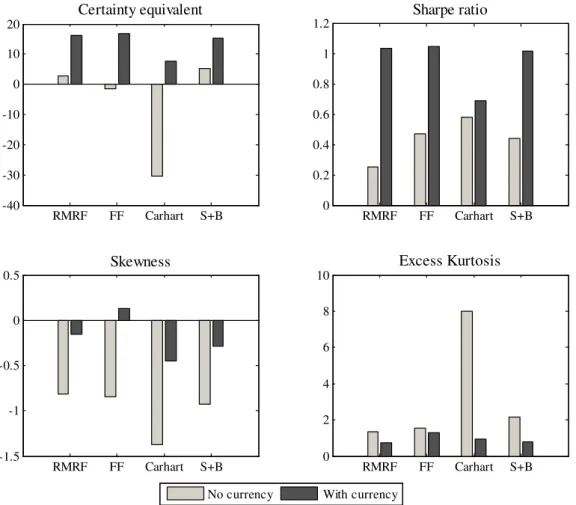
Figure 1.4 shows how complementing a portfolio policy with investments

in the currency market contributes to performance, including kurtosis

and skewness. The currency strategies increase Sharpe ratios and

cer-tainty equivalents and, most notably, they also reduce substantially the

excess kurtosis and left-skewness of diversi…ed portfolios.

Our results make it hard to reconcile the economic value of currency

investing with the existence of some set of risk factors that drives returns

in currencies and other asset classes. The substantial increases in Sharpe

ratios combined with the lower crash risk indicate that there is either

a speci…c set of risk factors in the currency market or that currency

returns have been anomalous throughout our sample.

1.7 Speculative capital

We cannot justify the pro…tability of our currency strategy as

compen-sation for risk. The obvious alternative explanation is market

ine¢-ciency. This might arise due to insu¢cient arbitrage capital, possibly

because strategies exploring the cross section of currency returns were

not well known. Jylhä and Suominen (2011) …nd carry returns explain

hedge fund returns controlling for the other factors proposed by Fung

and Hsieh (2004) and that growth in hedge fund speculative capital is

(55)

Following Jylhä and Suominen (2011), we run an OLS regression of

the returns of the optimal strategy on hedge fund assets under

man-agement scaled by the monetary aggregate M2 of the 11 currencies in

their sample (AU M=M2) and new fund ‡ows ( AU M=M2):23 _The

re-gression uses the out-of-sample returns, after transaction costs, of the

optimal strategy from 1996:03 to 2008:12 as the dependent variable. The

estimated coe¢cients (and t-statistics in parenthesis) are:

rp;t = 0:08 1:47 (AU M_M₂ )t 1 +3:56 ( AU M_M₂ )t

(4:29) ( 3:23) (0:36)

The new ‡ow of capital to hedge funds is not signi…cant in the

re-gression but the estimated coe¢cient has the correct sign. The level of

hedge fund capital predicts negatively the returns of the optimal

strat-egy. With a t-statistic of -3.23, this provides convincing evidence that

the returns of the diversi…ed currency strategy are an anomaly that is

gradually being corrected as more hedge fund capital exploits it.

This opens the question whether the large returns of the strategy

are likely to continue going forward. We note that in the last three

years of our sample (2009-2011) the strategy produces a Sharpe ratio of

0.82, lower than its historical average but still an impressive performance

(though not much di¤erent than the stock market in the same period).

2 3_{We thank Matti Suominen for providing us the time series of AUM/M2. See their}

(56)

1.8 Conclusion

Diversi…ed currency investments using the information of momentum,

yield di¤erential, and reversal, outperform the carry trade substantially.

This outperformance materializes in a higher Sharpe ratio and in less

severe drawdowns, as reversal and momentum had large positive returns

when the carry trade crashed. The performance of our optimal currency

strategy poses a problem to peso explanations of currency returns.

Our optimal currency portfolio picks stable coe¢cients for the

rel-evant currency characteristics and, by dealing with transaction costs,

outperforms naive benchmarks proposed in the literature.

The economic performance of the optimal currency portfolio cannot

be explained by risk factors or time-varying risk. This suggests market

ine¢ciency or, at least, that the right risk factors to explain currency

momentum and reversal returns have not been identi…ed yet. Investing

in currencies signi…cantly improves the performance of diversi…ed

port-folios already exposed to stocks and bonds. So currencies either o¤er

exposure to some set of unknown risk factors or have anomalous returns.

The most convincing explanation for the returns of our optimal

di-versi…ed currency portfolio is that it constitutes an anomaly – one which

is being gradually arbitraged away as speculative capital increases in the

(57)

Strategy Max Min Mean std kurt skew SR CE fd 15.91 -25.39 19.23 19.47 4.48 -1.23 0.99 18.97 mom 17.31 -11.60 8.01 14.23 1.80 0.21 0.56 11.61 rev 8.38 -11.31 3.09 8.72 2.24 -0.26 0.36 8.95 sign 21.29 -30.11 17.96 18.74 7.35 -0.90 0.96 18.29

ca 2.79 -3.47 0.61 3.86 1.24 -0.44 0.16 7.59 q 2.02 -2.32 0.12 1.79 4.44 -0.74 0.07 7.34 fd, mom, rev, sign 56.83 -32.78 44.30 32.89 5.54 0.66 1.35 34.72

All 60.38 -25.56 45.28 33.70 5.10 0.60 1.34 34.85