A Work Project presented as part of the requirements for the Award of a Master Degree in Economics from the NOVA – School of Business and Economics – and from the INSPER.
Strategic Asset Allocation in Brazil
André Filipe Barreto Morais
24644
A Project carried out on the Double Degree Program in Economics, under the supervision of:
João Manuel Amaro de Matos and Marco Antônio Cesar Bonomo.
Strategic Asset Allocation in Brazil
Abstract
We study the impact of asset returns’ predictability on optimal portfolio allocation,
considering investors concerned with a steady flow of long-term consumption. Relying on a
monthly database for 2006-2016, the analysis focuses on the Brazilian context covering
returns on (1) a real short-term asset, (2) a long-term asset, (3) a Brazilian stock index, and
five other state variables. Predictability of long-term assets returns has a significant impact on
their overall optimal demand. In addition, by using the S&P500 index we show that foreign
stocks are more predictable than the Brazilian index for moderately conservative investors.
JEL Classification: G11
Keywords: Intertemporal hedging demand; Portfolio Choice; Predictability; Strategic asset
allocation
Acknowledgments
I am tremendously indebted to my supervisors, João Amaro de Matos and Marco Antônio
Cesar Bonomo, for all the recommendations, motivation and suggestions. I am also
enormously grateful for the computational support provided by Professor Marco Lyrio.
I dedicate this work to those who have always been with me during this fascinating academic
1 Introduction
Harry Markowitz (1952) pioneered the analysis of quantitative finance with the
unprecedented article Portfolio Selection. In his work, the author shows the importance of the process of asset allocation through portfolio diversification. The mean-variance analysis of
Markowitz, despite having proved to be a robust tool in the process of asset allocation and be
widely used, has shown some inconsistencies with long-term asset allocation. This theory is
based on the assumption that investors are only concerned with the wealth distribution a
period ahead. Thus, the model is static and does not capture the investor’s concern to maintain
a flow of long-term consumption provided by its wealth.
Markowitz’s model should be extended in order to take into consideration the
long-term allocation process, namely the investors’ need to reduce the risk of having their
consumption affected over time. Paul Samuelson (1969) and Robert Merton (1969, 1971)
started developing that line of research in the context of multi-period models. Because they do
not present closed form solution, very complex numerical methods are necessary, which, for a
long time, made the use of these models unviable. The computational revolution in the 1990s,
alongside with the recent developments in numerical methods, made the implementation of
multi-period models more appealing in the recent past.
Solutions of multi-period asset allocation models may differ significantly from those
presented by static models, as summarized in Campbell and Viceira (2002). Particularly,
when investment opportunities are not constant over time, long-term investors are concerned
both with shocks to these opportunities and with shocks to their own wealth. In order to hedge
this exposure, long-term investors should seek an intertemporal demand for protection in
financial assets. This demand for protection is related to the agents’ degree of risk aversion.
Investors with relative risk aversion equal to one allocate their wealth purely myopically, not
agents seek for assets that increase in value in case of deterioration in investment
opportunities. These assets behave as insurance against the risks of falling returns on wealth.
Investment opportunities are not constant over time. Campbell (1999), Fama and
French (1989), among others, provide empirical evidence supporting that. The real rate of
short-term interest has changed over time, but, at the same time, the excess returns on stocks
and bonds also show some predictability in their dynamics. The most important aspect in
these findings is the mean reversion tendency of stocks in the long-run. This feature reflects
the different perception of risk that short and long-term investors have.
In order to meet the long-term analysis using the mean-variance model, one could
calculate long-run variances and apply them in the static model. However, such a solution
would only serve investors who are only concerned with the average and volatility of their
wealth in a single period of time. And yet, this investor would be limited to making a single
allocation for that period, without the opportunity for rebalancing it over time.
Hereupon, this article replicates the dynamic model proposed by Campbell, Viceira,
and Chan (2003). In particular, we study how the predictability and persistence of some
selected Brazilian assets’ returns affect the long-term wealth distribution of an investor who
values a constant stream of consumption, and considers, in his decision, the variability of
investment opportunities over time.
2 The Model
2.1 Securities
The model assumes that n securities are available to invest, and investors can distribute their wealth, after consumption, among them. 𝑅",$%& is the real portfolio return, 𝛼(,$
is the portfolio weight on asset 𝑖, and 𝑅&,$%& is the benchmark real return. We use a real short-term asset return as a benchmark and, then, calculate excess returns by using it. Though, the
𝑅",$%&= 𝛼(,$ 𝑅(,$%&− 𝑅&,$%& + 𝑅&,$%&
-(./
. (1)
2.2 State variables dynamics
Following Campbell et al. (2003), we assume a first-order vector autoregressive process VAR(1) to capture the dynamics of the relevant state variables1. Hereby, the vector of
log excess returns, 𝒙𝒕%𝟏, is defined in the following way:
𝒙𝒕%𝟏≡
𝑟/,$%&− 𝑟&,$%&
𝑟6,$%&− 𝑟&,$%&
⋮ 𝑟-,$%&− 𝑟&,$%&
, (2)
where 𝑟(,$%& ≡ log (𝑅(,$%&). In this article, 𝑟&,$%& is the real short-term return, 𝑟/,$%& is the real
return on nominal bonds, or long-term assets, and 𝑟6,$%& is the real stock index return. The system is going to include three other state variables, 𝑠$%&. Placing 𝑟&,$%&, 𝑥$%&, and 𝑠$%&
together, we get a 𝑚×1 vector, the state vector:
𝒛𝒕%𝟏≡ 𝑟&,$%&
𝑥$%&
𝑠$%&
. (3)
The first-order vector autoregressive system is equated in the following matrix form:
𝒛𝒕%𝟏= 𝚽𝟎+ 𝚽𝟏𝑧$+ 𝒗𝒕%𝟏, (4)
𝒗𝒕%𝟏~𝑁(0, ΣL),
(5) 𝚺𝐯≡ 𝑉𝑎𝑟$ 𝒗𝒕%𝟏 =
𝜎&/ 𝝈𝟏𝒙S 𝝈𝟏𝒔S
𝝈𝟏𝒙 𝚺𝒙𝒙 𝚺𝒙𝒔S
𝝈𝟏𝒔 𝚺𝒙𝒔 𝚺𝒔𝒔
,
where, 𝚽𝟎 is the 𝑚×1 matrix of interceps, 𝚽𝟏 is the 𝑚×𝑚 slope coefficients matrix, and 𝒗𝒕%𝟏represents the shocks to the state variables. These shocks are independent and identically distributed (i.i.d.). Consequently, they can be cross-sectionally correlated, although they are homoscedastic and independently distributed over time. By using a VAR system, we can
1
analyse the dependence of expected asset returns on their previous values, even as on other
variables that show to be good predictors.
Assuming these shocks are homoscedastic, it does not allow the state variables to
predict changes in risk. Portfolio choice is only affected by their predictive power in expected
returns. However, in the late 1980’s and early 1990’s some authors2 have studied the
capability of the state variables in predicting risk, and found out that these variables had little
power in predicting risk. The state variables had bigger effects in predicting expected returns,
dominating the former effect.
2.3 Preferences
Here, the investor is going to be assumed of having recursive Epstein-Zin (1989, 1991)
preferences. The convenience this model of utility holds is held by its characteristic that
allows to separate the definition of relative risk aversion from elasticity of intertemporal
substitution. They are not necessarily the inverse of each other anymore, like in the older
power utility model, 𝛾 ≠ 𝜓X&. Then, the utility function is expressed below:
𝑈 𝐶$, 𝐸$ 𝑈$%& = 1 − 𝛿 𝐶$ &X]
^ + 𝛿 𝐸 $ 𝑈$%&
&X] & ^
^ &X]
, (6)
where 𝐶$ represents consumption at time 𝑡, 𝛾 holds for relative risk aversion, 𝜓 is the
elasticity of intertemporal substitution, 𝛿 is the time discount factor, 𝜃 is equal to (&X])
(&Xabc), and
𝐸$(∙) is the conditional expectation operator.
At time 𝑡, agents use all relevant information in order to make an optimal
consumption and portfolio allocation over time. The investor is constrained to an
intertemporal budget constraint:
𝑊$%&= 𝑊$− 𝐶$ 𝑅",$%&, (7)
2
where 𝑊$ is wealth at time 𝑡. The Euler equation for consumption, subject to the intertemporal budget constraint, derived by Epstein and Zin (1989 and 1991) is expressed by:
𝐸$ 𝛿
𝐶$%&
𝐶$ Xa& ^
𝑅",$%&X &X^ 𝑅(,$%& = 1. (8)
This equation is set for an asset 𝑖, and also for the portfolio. Consumption and portfolio
decisions of investors must satisfy this Euler equation (8). When investment opportunities do
not vary over time, the equilibrium decision should be a constant consumption-wealth ratio,
and investors optimize their portfolios myopically. The allocation decision is made as if the
investment horizon is only one period ahead. However, when investment opportunities vary
over time, there are no exact analytical solutions to this equation, except for certain values of
𝛾 and 𝜓. Giovannini and Weil (1989) showed that, with 𝛾 = 1, the investor should follow a
myopic rule, and that he chooses a constant ratio of consumption-wealth equal to (1 − 𝛿)
when 𝜓 = 1. Though, when 𝛾 = 1, a choice for consumption relative to wealth is not
constant, unless 𝜓 = 1, and likewise, with 𝜓 = 1, the optimal allocation is not myopic, unless
𝛾 = 1. This is the case of the log utility investor, 𝛾 = 𝜓 = 1.
3 Methodology of the solution
3.1 An approximation
In this framework, we are going to use log returns. Campbell and Viceira (1999, 2001)
got to the following expression of log portfolio returns3, accurate for continuous time:
𝑟",$%&= 𝑟&,$%&+ 𝜶𝒕S𝒙𝒕%𝟏+
1 2𝜶𝒕
S 𝝈 𝒙 𝟐− 𝚺
𝒙𝒙𝜶𝒕 . (9)
The vector 𝝈𝒙𝟐 ≡ 𝑑𝑖𝑎𝑔(𝚺𝒙𝒙) contains the variances of excess returns.
The budget constraint in (7) is not linear. According to Campbell (1993, 1996),
log-linearization around the unconditional mean of the log consumption-wealth ratio obtains
3
Δ𝑤$%&≈ 𝑟",$%&+ 1 −
1
𝜌 𝑐$− 𝑤$ + 𝑘, (10)
where Δwr%& is the difference between 𝑤$%& and 𝑤$, 𝜌 ≡ 1 − exp (𝐸 𝑐$− 𝑤$ ) and 𝑘 ≡
log 𝜌 + 1 − 𝜌 log (&Xv)
v . As consumption is optimally chosen by the investor, 𝜌 depends
on the optimal level of 𝑐$ relative to 𝑤$, and, thus, is endogenous. This form of budget
constraint is exact if the elasticity of intertemporal substitution is equal to one and, in this
case, 𝑐$− 𝑤$ is a constant equal to (1 − 𝛿).
By applying a second-order Taylor expansion to the Euler equation (8) around the
conditional means of Δ𝑐$%&, 𝑟",$%& and 𝑟(,$%&, one obtains a loglinearized Euler equation that
becomes exact if consumption and return on assets have lognormal joint distribution (𝜓 = 1).
Hence, we get to a transformed log linearized Euler equation as follows:
Er 𝑟(,$%&− 𝑟&,$%& + &
/𝑉𝑎𝑟$(𝑟(,$%&− 𝑟&,$%&) = ^
a 𝜎(,xXy,$− 𝜎&,xXy,$ + 𝛾 𝜎(,",$− 𝜎&,",$ − (𝜎(,&,$− 𝜎&,&,$), (11)
where,
𝜎(,xXy,$= 𝐶𝑜𝑣 𝑟(,$%&, 𝑐$%&− 𝑤$%& , 𝜎&,xXy,$ = 𝐶𝑜𝑣 𝑟&,$%&, 𝑐$%&− 𝑤$%& , 𝜎(,",$= 𝐶𝑜𝑣 𝑟(,$%&, 𝑟",$%& ,
𝜎&,",$= 𝐶𝑜𝑣 𝑟&,$%&, 𝑟",$%& , 𝜎(,&,$= 𝐶𝑜𝑣 𝑟(,$%&, 𝑟&,$%& , 𝑎𝑛𝑑 𝜎&,&,$= 𝑉𝑎𝑟 𝑟&,$%& .
Left-hand part of the equation (11) is the risk premium on asset 𝑖 over asset 1, adjusted for
Jensen’s Inequality by adding half of the excess return variance. This equation relates the risk
premium of asset 𝑖 to its excess of covariance with consumption growth, to its excess of
covariance with the return on the portfolio, and to the covariance of its excess return with the
return on asset 1 (the last term is eliminated from the equation when asset 1 presents no risk).
Since consumption growth and portfolio return are endogenous, this equation is a first-order
condition that describes the optimal solution and not a solution on its own.
3.2 Solving the approximate model
In order to solve the model, Campbell and Viceira (2002) assume that the optimal rule
𝛂r= 𝑨•+ 𝑨&𝒛$, (12)
cr− 𝑤$= 𝑏•+ 𝐁&S𝒛$+ 𝒛$S𝑩/𝒛$. (13)
The optimal rule for the portfolio is thus linear in the VAR state vector, however the optimal
rule for consumption is quadratic. 𝑨𝟎 (𝑛 − 1)×1, 𝑨𝟏 (𝑛 − 1)×𝑚, 𝑏𝟎 1×1, 𝑩𝟏 𝑚×1, and
𝑩𝟐 𝑚×𝑚 are matrices of constant coefficients to be determined. This is the generalization of
the solution obtained by Campbell and Viceira (1999) for the multivariate case. It is
noteworthy that only 𝑚 +„…X„
/ elements of 𝑩/ are to be determined.
In order to validate equations (12) and (13) and obtain the solution of the parameters,
the conditional moments appearing in (11) are written as functions of the VAR parameters
and the unknown parameters of (12) and (13). Next, we solve this resulting equation for the
parameters that satisfy (11). Consequently, the conditional expectation of equality (11) is:
Er 𝒙$%& +
1
2𝑉𝑎𝑟$ 𝒙𝒕%𝟏 = 𝑯𝒙𝚽𝟎+ 𝑯𝒙𝚽𝟏𝒛𝒕+ 1 2𝝈𝒙
𝟐.4 (14)
Campbell et al. (2003) show that the three conditional moments on the right-hand side of equation (11) can be written as linear functions of the state variables:
𝝈xXy,$− 𝜎&,xXy,$𝒍 ≡ 𝜎(,xXy,$− 𝜎&,xXy,$ (./,…,-= 𝚲𝟎+ 𝚲𝟏𝒛𝒕 , (15)
𝝈",$− 𝜎&,",$𝒍 ≡ 𝜎(,",$− 𝜎&,",$ (./,…,-= 𝚺𝒙𝒙𝜶𝒕+ 𝝈𝟏𝒙, (16)
𝝈&,$− 𝜎&,&,$𝒍 ≡ 𝜎(,&,$− 𝜎&,&,$ (./,…,-= 𝝈𝟏𝒙, (17)
where 𝒍is a vector of ones.
3.3 Optimal Portfolio Choice
After the log linearized Euler equation (11) being solved for the optimal portfolio rule:
𝜶𝒕 =
1 𝛾𝚺𝒙𝒙
X𝟏 𝐸
$ 𝑥$%& +
1
2𝑉𝑎𝑟$ 𝑥$%& + (1 − 𝛾)𝝈𝟏𝒙 + 1 𝛾𝚺𝒙𝒙
X𝟏 −𝜃
𝜓(𝝈xXy,$− 𝜎&,xXy,$𝒍) . (18)
𝐸$ 𝑥$%& +&
/𝑉𝑎𝑟$ 𝑥$%& and (𝝈xXy,$− 𝜎&,xXy,$𝒍) are linear functions of 𝒛𝒕 in (14) and (15),
respectively. The optimal portfolio choice is expressed as the sum of two components.
4
The first term on the right of (18) is the myopic component. When the benchmark
asset is considered not risky (𝝈𝟏𝒙= 0), the myopic allocation is ruled essentially by the
Sharpe ratio (SR) of the risky assets: the vector of expected excess returns is adjusted by the
inverse of the variance-covariance matrix of returns on risky assets and the inverse of the
relative risk aversion coefficient. If asset 1 is risky, investors with 𝛾 ≠ 1 adjust their
allocation by a term (1 − 𝛾)𝝈𝟏𝒙. This component does not depend on 𝜓.
The second term on the right of (18) represents the demand for protection. In this
model, investment opportunities vary over time because the expected returns of the assets
depend on the state variables. An investor who is more risk averse than a log utility investor,
will seek protection against adverse changes in investment opportunities (Merton 1969,
1971). He will optimize his portfolio by having strategic positions in some assets. A
logarithmic investor optimizes his allocation purely myopically, having no hedging demand.
If 𝛾 = 1, then 𝜃 = 0, therefore, the protection component disappears. Yet, when investment
opportunities are constant, the demand for protection is zero for every level of risk aversion,
corresponding to a VAR model with just a constant term.
By replacing (14) and (15) into (18):
𝛂𝐭≡ 𝑨𝟎+ 𝑨𝟏𝒛𝒕, (19)
where,
𝑨𝟎= 1 𝛾 𝚺𝒙𝒙
X𝟏 𝑯 𝒙𝚽𝟎+
1 2𝝈𝒙
𝟐+ 1 − 𝛾 𝝈
𝟏𝒙 + 1 −
1 𝛾 𝚺𝒙𝒙
X𝟏 −𝚲𝟎
1 − 𝜓 , (20)
𝑨𝟏=
1 𝛾 𝚺𝒙𝒙
X𝟏𝑯
𝒙𝚽𝟏+ 1 −
1 𝛾 𝚺𝒙𝒙
X𝟏 −𝚲𝟏
1 − 𝜓 . (21)
Equation (19) confirms the initial assumption made by Campbell et al. (2003) for the initial guessing of the optimal portfolio rule. Coefficients matrices 𝑨𝟎 and 𝑨𝟏 show as functions of the parameters that describe preferences and the dynamics of the state variables, as well as of
note that the terms 1 −&
] in equations (20) and (21) picture the effect of intertemporal
protection on optimal portfolio choice. Therefore, the demand for intertemporal protection
affects the average allocation of the portfolio through 𝑨𝟎 and 𝑨𝟏, and the sensitivity of the optimal allocation to variations in the state variables through 𝑨𝟏.
Campbell et al. (2003) show that given 𝜌, the coefficient matrices X𝚲𝟎
&Xa and X𝚲𝟏 &Xa
are independent of the intertemporal elasticity of substitution 𝜓. Hence, the optimal portfolio
rule is independent for any 𝜓 given 𝜌. 𝜓 only affects portfolio choice as it defines 𝜌.
4 Empirical Application
Previous section presented the academical background of strategic asset allocation.
Here, such a set-up is used to assess how investors, who differ in their preferences for
consumption and risk aversion, distribute their portfolio among the available assets provided
by the model: a real short-term asset (STA), a long-term asset (LTA), and a stock. The VAR
system describes the dynamics of investment opportunities using a real short-term asset
return, an excess-return of a stock-market index, an excess-return of a long-term asset, and
other state variables that help to forecast these excess-returns. Optimal allocation of the
portfolio is computed for different levels risk-aversion 𝛾. Assuming that 𝜓 = 1, 𝑐$− 𝑤$=
1 − 𝛿5, and 𝛿 = 0,956 in annual terms, implies that the parameter 𝜌 = 𝛿7.
4.1 Data Description
For the purpose of this study, log returns of portfolio assets, and other state variables
are necessary. Our sample covers January 2006 to December 2016, using monthly frequency.
In order to construct monthly log returns of the real short-term asset (STA), we obtained the
5
When 𝜓 = 1, Campbell et al. (2003) show that consumption-wealth ratio equals 1 − 𝛿. 6
This value, 0,95, is obtained by 𝛿 = 𝑒X‘’, where 𝑠𝑟 is the mean average of the CDI rate of return for the
considered period. We get the same value for 𝛿 when we consider the IDkA Pre 3M return instead. 7
accumulated monthly nominal return over the CDI rate, which is a daily average of the
overnight interbank loans in Brazil, adjusted by inflation – 𝑟x“(. For the monthly log
excess-return of stock-market index (Stock), we gathered monthly nominal excess-returns over the Ibovespa
index 𝑟(”•–, monthly nominal returns over the IbrX index 𝑟(”’—, and monthly nominal returns
over the S&P 500 index plus the exchange-rate returns between the U.S. Dollar and the
Brazilian Real 𝑟‘"— (SPXBRL). Monthly log excess returns of the long-term asset (LTA) were constructed using monthly nominal returns of a set of indexes that measure the behaviour of
synthetic portfolios of Brazilian federal securities with constant term8: IDkA Pre 3M, 𝑟6„
(three months), IDkA Pre 1A, 𝑟&˜ (one year), IDkA Pre 2A, 𝑟/˜ (two years), IDkA Pre 3A,
𝑟6˜ (three years), IDkA Pre 5A, 𝑟™˜ (five years), IDkA IPCA 2A, 𝑟("xš/˜ (two years), IDkA IPCA 3A, 𝑟("xš6˜ (three years), IDkA IPCA 5A, 𝑟("xš™˜ (five years). The 3 last indexes can be analysed as inflation-indexed bonds. Note that IDkA Pre 3M, 𝑟6„, is also used as an alternative for the monthly log returns of the real short-term asset. Subsequently, the
12-month accumulated Ibovespa dividend-yield, 𝑠“X", the yield-spread between the IDkA Pre
5A and the IDkA Pre 3M, 𝑠‘"’›š“, the nominal return over the CDI, 𝑠˜x“(, the nominal return
over the IDkA Pre 3M, 𝑠˜6„, the Emerging Markets Bond Index9 (EMBI +), 𝑠›„”(, and, finally, the 12-month accumulated return over the Brazilian Institute of Geography and
Statistics’ (IBGE) price index (IPCA-IBGE), 𝑠("xš, were the state variables chosen to predict
the returns10. All the variables adjusted by inflation used IPCA-IBGE.
In the next sections, we use combinations of these log returns and state variables.
8
Since January 2006, these indexes are constructed by the Brazilian Association of Financial and Capital Markets (ANBIMA).
9
The EMBI + is an index, created by JPMorgan, based on debt securities issued by emerging countries. It shows the financial returns obtained each day by a selected portfolio of securities from these countries. The unit of measure is the base point. Ten basis points are equivalent to one-tenth of 1%. Points show the difference between the rate of return of emerging-market securities and that offered by securities issued by the US Treasury. This difference is the spread, or the sovereign spread, which is also known by risk of Brazil.
10
𝑠“X", 𝑠‘"’›š“, and 𝑠˜ are variables that have been identified as good return predictors by authors such as,
respectively, Fama and Schwert (1977), Campbell (1987), and Glosten et al. (1993). Moreover, 𝑠›„”(, and
4.2 Sample Analysis
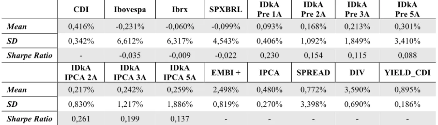
Table 1.1 and Table 1.2 show the first and second moments for the historical series of
the variables introduced before. In Table 1.1, stock returns and LTA returns are in the excess
form over the CDI return. These same returns, in Table 1.2, are in the excess form over the
IDkA Pre 3M return. Sample statistics are in percentage and in monthly frequency. Log mean
excess-returns are adjusted by half of the variance to accommodate for Jensen’s inequality. In
both tables, LTA have the highest log mean excess-return and the lowest volatility, therefore,
they also hold the highest Sharpe ratios, contrary to Campbell, et al. (2003) where stocks had the highest Sharpe ratio.
Table 1.1 – Sample Statistics (Excess returns over CDI return)
CDI Ibovespa Ibrx SPXBRL IDkA Pre 1A
IDkA Pre 2A
IDkA Pre 3A
IDkA Pre 5A
Mean 0,416% -0,231% -0,060% -0,099% 0,093% 0,168% 0,213% 0,301%
SD 0,342% 6,612% 6,317% 4,543% 0,406% 1,092% 1,849% 3,410%
Sharpe Ratio - -0,035 -0,009 -0,022 0,230 0,154 0,115 0,088
IDkA IPCA 2A
IDkA IPCA 3A
IDkA
IPCA 5A EMBI + IPCA SPREAD DIV YIELD_CDI
Mean 0,217% 0,242% 0,259% 2,498% 0,480% 0,772% 3,590% 0,895%
SD 0,830% 1,217% 1,886% 0,819% 0,270% 3,398% 0,690% 0,186%
Sharpe Ratio 0,261 0,199 0,137 - - - - -
Table 1.2 – Sample Statistics (Excess returns over IDkA Pre 3M return) IdkA Pre
3M Ibovespa Ibrx SPXBRL
IDkA Pre 1A
IDkA Pre 2A
IDkA Pre 3A
IDkA Pre 5A
Mean 0,429% -0,244% -0,073% -0,112% 0,081% 0,155% 0,200% 0,288%
SD 0,354% 6,611% 6,314% 4,545% 0,372% 1,067% 1,827% 3,391%
Sharpe Ratio - -0,037 -0,011 -0,025 0,216 0,145 0,109 0,085
IDkA IPCA 2A
IDkA IPCA 3A
IDkA IPCA
3A EMBI + IPCA SPREAD DIV YIELD_3M
Mean 0,204% 0,229% 0,246% 2,498% 0,480% 0,772% 3,590% 0,908%
SD 0,802% 1,190% 1,864% 0,819% 0,270% 3,398% 0,690% 0,203%
Sharpe Ratio 0,254 0,192 0,132 - - - - -
It is worth noting that both of the previous tables have a negative log mean
excess-return for stocks (Ibovespa, IbrX, and S&P 500). They have also the highest volatility.
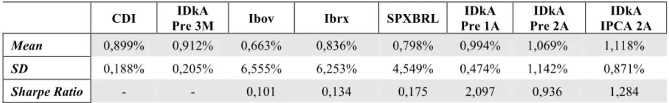
Table 2 contains mean nominal returns for CDI, IdkA Pre 3M, Ibovespa, SPXBRL,
subsequent exercises. These returns are not in the log form, therefore, they were not corrected
by half the variance. They are also not presented in the excess-return form.
Table 2 – Nominal Returns
CDI IDkA
Pre 3M Ibov Ibrx SPXBRL
IDkA Pre 1A IDkA Pre 2A IDkA IPCA 2A
Mean 0,899% 0,912% 0,663% 0,836% 0,798% 0,994% 1,069% 1,118%
SD 0,188% 0,205% 6,555% 6,253% 4,549% 0,474% 1,142% 0,871%
Sharpe Ratio - - 0,101 0,134 0,175 2,097 0,936 1,284
Once again, it can be seen that Ibovespa shows to be the worst investment, ex-post.
This is clear when we analyse Figure 1. This graph shows the result of an investment of
R$100,00 in the beginning of January 2006 in each of the following eight assets: CDI, IDkA
Pre 3M, Ibovespa, Ibrx, SPXBRL, IDkA Pre 1A, IDkA Pre 2A, and IDkA IPCA 2A.
Figure 1
In December 2016 the CDI strategy results in R$325,95, the IDkA Pre 3M strategy results in
R$331.49, the Ibovespa strategy results in R$180,02, the Ibrx strategy results in R$231,53,
and, even taking into account the exchange rate risk, the S&P500 strategy yields R$249,58,
exceeding both Brazilian stock-market indexes. All three assets that follow outperformed
STA and stocks: IDkA Pre 1A, IDkA Pre 2A, and IDkA IPCA 2A. In December 2016, the
IDkA Pre 1A strategy results in R$368,34, the IDkA Pre 2A strategy results in R$403,61, the
IDkA IPCA 2A strategy results in R$432,02. 0 100 200 300 400 500 Ja n -06 Ju l-06 Ja n -07 Ju l-07 Ja n -08 Ju l-08 Ja n -09 Ju l-09 Ja n -10 Ju l-10 Ja n -11 Ju l-11 Ja n -12 Ju l-12 Ja n -13 Ju l-13 Ja n -14 Ju l-14 Ja n -15 Ju l-15 Ja n -16 Ju l-16
Investing R$100 in January 2006
CDI IDkA Pre 3M Ibovespa Ibrx
4.3 VAR Estimation
There were made 391 combinations containing a real short-term asset, a long-term
asset and a stock (Brazilian stock or foreign stock), and three other state variables by using
the data presented in Section 4.1. Afterwards, for the purpose of this analysis, we selected
four types of combinations: one that includes a long-term asset and a Brazilian stock-market
index; a Brazilian stock-market index and a foreign equity index; a long-term
inflation-indexed asset and a Brazilian stock-market index; and, finally, a combination that contains a
long-term asset, a Brazilian stock-market index, and the same state variables used by
Campbell et al. (2003), which are the 12-month accumulated dividend yield, the spread between a long-term asset and a short-term asset, and the benchmark nominal return. The
selection process consisted in selecting the combinations with more statistical significant
coefficients and highest excess-returns’ R-squared in their VAR estimations. They are going
to be named combination 1, combination 2, combination 3 and combination 4, respectively.
Tables 3 and 4 display the estimated VAR parameters and the covariance structure of
unexpected returns, respectively. Tables 3 exhibit the estimated coefficients of the VAR
setting, as well as their t-statistics, in parentheses, and the R-squared statistics. Tables 4 show,
in the main diagonal, the standard deviations of the unexpected returns multiplied by 100, and
the upper-diagonal elements are the cross-correlation coefficients of unexpected returns.
4.3.1 VAR Estimation – Combination 1
In this combination, it was used the CDI real return as a real short-term variable, the
IDkA Pre 1A excess return over CDI as a LTA, the Ibovespa excess-return over CDI as a
stock-market index, and three other state variables: the 12-month accumulated dividend yield,
the EMBI + spread, and the CDI nominal return. This is the first-type combination with more
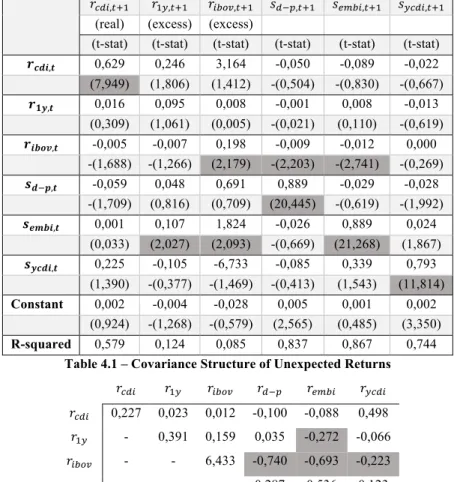
In Table 3.1, the second column presents the equation of the real short-term asset,
where the only variable that explains its future returns is its one-year lagged returns11.
Third column of Table 3.1 shows the equation of the LTA, 𝑟&˜,$%&. Lagged LTA returns are not statistically significant in predicting its future returns. The EMBI + spread has
a coefficient with t-statistics greater than 2, being the only variable with predictive power in
this equation.
Table 3.1 – VAR Parameters
𝑟x“(,$%& 𝑟&˜,$%& 𝑟(”•–,$%& 𝑠“X",$%& 𝑠›„”(,$%& 𝑠˜x“(,$%&
(real) (excess) (excess)
(t-stat) (t-stat) (t-stat) (t-stat) (t-stat) (t-stat)
𝒓𝒄𝒅𝒊,𝒕 0,629 0,246 3,164 -0,050 -0,089 -0,022
(7,949) (1,806) (1,412) -(0,504) -(0,830) -(0,667)
𝒓𝟏𝒚,𝒕 0,016 0,095 0,008 -0,001 0,008 -0,013
(0,309) (1,061) (0,005) -(0,021) (0,110) -(0,619)
𝒓𝒊𝒃𝒐𝒗,𝒕 -0,005 -0,007 0,198 -0,009 -0,012 0,000
-(1,688) -(1,266) (2,179) -(2,203) -(2,741) -(0,269)
𝒔𝒅X𝒑,𝒕 -0,059 0,048 0,691 0,889 -0,029 -0,028
-(1,709) (0,816) (0,709) (20,445) -(0,619) -(1,992)
𝒔𝒆𝒎𝒃𝒊,𝒕 0,001 0,107 1,824 -0,026 0,889 0,024
(0,033) (2,027) (2,093) -(0,669) (21,268) (1,867)
𝒔𝒚𝒄𝒅𝒊,𝒕 0,225 -0,105 -6,733 -0,085 0,339 0,793 (1,390) -(0,377) -(1,469) -(0,413) (1,543) (11,814)
Constant 0,002 -0,004 -0,028 0,005 0,001 0,002 (0,924) -(1,268) -(0,579) (2,565) (0,485) (3,350)
R-squared 0,579 0,124 0,085 0,837 0,867 0,744
Table 4.1 – Covariance Structure of Unexpected Returns
𝑟x“( 𝑟&˜ 𝑟(”•– 𝑟“X" 𝑟›„”( 𝑟˜x“(
𝑟x“( 0,227 0,023 0,012 -0,100 -0,088 0,498
𝑟&˜ - 0,391 0,159 0,035 -0,272 -0,066
𝑟(”•– - - 6,433 -0,740 -0,693 -0,223
𝑟“X" - - - 0,287 0,536 0,123
𝑟›„”( - - - - 0,309 0,122
𝑟˜x“( - - - 0,094
Fourth column of Table 3.1 presents the log equation of the Ibovespa excess-return
over the CDI. The remark addressed by Campbell et al. (2003) is also valid here: stock’s excess-returns are difficult to predict – this equation has the lowest R-squared, 0,085. Only
lagged stock returns and lagged risk of Brazil spread have predictive power.
11
Among these two excess-returns’ equations the one that has the highest R-squared is
the one of the LTA. Although, the number of variables that help to predict these asset returns
is higher in the Ibovespa equation, with two statistically significant variables. The first two
equations have only one statistically significant variable each.
Last three columns show the results of the estimated parameters for the state variables
equations. Each of these three equations is well described by an AR (1) process. Their own
lagged coefficients are positive and close to one, thus, presenting a dynamic persistence. The
third state variable, CDI nominal return, has the lowest coefficient, 0,793.
Table 4.1 shows the covariance structure of the VAR system innovations. Unexpected
returns of Ibovespa are negatively correlated with shocks to its 12-month accumulated
dividend yield. This is in line with what was found in previous empirical research promoted
by authors such as Campbell (1991), Campbell and Viceira (1999), and Stambaugh (1999).
Shocks to Ibovespa returns are also negatively correlated with shocks to the EMBI + spread
state variable, and with shocks to the CDI nominal returns. Finally, LTA unexpected returns
are negatively correlated with shocks to the EMBI + spread.
4.3.2 VAR Estimation – Combination 2
Combination 2 differs from combination 1 in the real short-term asset and in the
long-term asset. They are substituted, respectively, by the log return of the IDkA Pre 3M and by
the log excess-return of the S&P 500 over IDkA Pre 3M return.
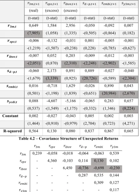
The second column of Table 3.2 presents the log equation of the foreign stock asset.
Its one-period lag and Brazilian stock’s one-period lag are the only coefficients statistically
significant in predicting real short-term asset’s returns.
Log equation of the foreign stock has only the 12-month accumulated dividend yield
coefficient statistically significant in predicting its returns. Its R-squared is the highest among
Ibovespa’s equation is statistically significant to predict its future returns. Among these
excess-returns, the one with highest R-squared is the real foreign stock.
Table 4.2 – VAR Parameters
𝑟6„,$%& 𝑟‘"—,$%& 𝑟(”•–,$%& 𝑠“X",$%& 𝑠›„”(,$%& 𝑠˜6„,$%&
(real) (excess) (excess)
(t-stat) (t-stat) (t-stat) (t-stat) (t-stat) (t-stat)
𝒓𝟑𝒎,𝒕 0,649 1,584 2,956 -0,050 -0,092 0,007
(7,905) (1,058) (1,335) -(0,505) -(0,864) (0,182)
𝒓𝒔𝒑𝒙,𝒕 -0,006 -0,132 -0,031 0,001 -0,005 -0,001
-(1,219) -(1,507) -(0,238) (0,228) -(0,785) -(0,627)
𝒓𝒊𝒃𝒐𝒗,𝒕 -0,007 0,052 0,203 -0,009 -0,012 -0,003
-(2,051) (0,870) (2,310) -(2,248) -(2,902) -(1,585)
𝒔𝒅X𝒑,𝒕 -0,060 2,173 0,891 0,889 -0,027 -0,040
-(1,679) (3,339) (0,925) (20,726) -(0,589) -(2,304)
𝒔𝒆𝒎𝒃𝒊,𝒕 0,016 -0,718 1,629 -0,026 0,890 0,043
(0,501) -(1,198) (1,839) -(0,651) (20,984) (2,670)
𝒔𝒚𝒄𝒅𝒊,𝒕 0,088 -4,607 -5,166 -0,065 0,283 0,657
(0,537) -(1,549) -(1,175) -(0,332) (1,346) (8,224)
Constant 0,002 -0,027 -0,043 0,005 0,002 0,003 (1,464) -(0,910) -(0,979) (2,704) (0,723) (4,271)
R-squared 0,564 0,130 0,080 0,837 0,867 0,665
Table 4.2 – Covariance Structure of Unexpected Returns
𝑟6„ 𝑟‘"— 𝑟(”•– 𝑟“X" 𝑟›„”( 𝑟˜6„
𝑟6„ 0,239 -0,058 -0,018 -0,064 -0,063 0,539
𝑟‘"— - 4,360 -0,103 0,114 0,130 0,102
𝑟(”•– - - 6,450 -0,736 -0,698 -0,230
𝑟“X" - - - 0,287 0,535 0,144
𝑟›„”( - - - - 0,309 0,127
𝑟˜6„ - - - 0,117
Last three columns comprise the results of the estimated parameters for the state
variables’ equations. Similarly, from combination 1, the three equations representing the state
variables are well described by an AR (1) process. Their lagged coefficients are positive and
close to one, presenting a dynamic persistence. Here, 𝑠˜6„ has the lowest coefficient, 0,657. Table 4.2 presents the covariance structure of the innovations of the VAR system.
Unexpected returns of Ibovespa are negatively correlated with shocks to the 12-month
IDkA Pre 3M, and with shocks to the risk of Brazil spread. Conversely, innovations to the
foreign stock are positively correlated with shocks to all three state variables.
Combination 3 does not have any lagged state variable with a statistical significant
coefficient in its log excess-returns’ equations. The same is true for combination 4, making it
hard to use these combinations, once it limits our ability to explain portfolio allocations.
4.4 Strategic Asset Allocations
In section 3.3 we show that the optimal allocation rule is linear in the vector of state
variables. Therefore, optimal allocation among the chosen assets varies over time. One way to
study this rule is to examine its mean and volatility. In order to analyse the magnitude of the
effects of the optimal allocation, we calculated the myopic allocations (tactical effect) for
each of these assets, as well as their demands for protection (strategic effect). Based on the
estimated VAR parameters and the cross-correlation of residuals, the optimal portfolios were
calculated for each of the four combinations of 𝜓 = 1, 𝛿 = 0,95 (at an annual frequency) and
𝛾 = 1, 𝛾 = 2, 𝛾 = 5, and 𝛾 = 20.
Both third and eighth columns in Table 5 show the portfolio allocation across the
STA, LTA or foreign stock, and Brazilian stock for a log utility investor holding combination
1 and combination 2, respectively. In this case, the investor is going to decide merely
myopically. When 𝛾 = 1, it can be seen from equation (18) that this allocation depends only
on the inverse of the variance-covariance matrix of unexpected excess-returns and on the
mean excess-returns. Therefore, the allocation decision is essentially based on the asset with
the best risk-return relationship, that is, the asset with the highest Sharpe ratio (SR, Table 1).
For combination 1, the myopic allocation when 𝛾 = 1 holds a long position in LTA of
6349,21%, a selling position in stock of 131,06% and a short position in STA of 6118,15% –
Table 5. The largest excess-return position is in the asset with the highest SR in absolute
value of the LTA to stock ratio of 48,45, probably due to the substantial positive estimated
correlation of 15,9% between unexpected returns on stocks and bonds, shifting the exposure
towards the asset with highest SR in absolute value.
Regarding combination 2, the myopic allocation when 𝛾 = 1 has a short position in
the foreign stock of 68,88%, a short position of 78,20% in the Brazilian stock and a long
position in the STA of 247,07%. The largest excess-return’s position is in the asset with the
highest absolute value in the SR, which is the Ibovespa, 0,037, compared to the -0,025 foreign
stock’s SR. Here, the foreign stock to Brazilian stock ratio is 0,88.
Table 5 – Mean Asset Demands for Combination 1 and Combination 2 (%)
Combination 1 Combination 2
Asset γ=1 γ=2 γ=5 γ=20 Asset γ=1 γ=2 γ=5 γ=20 Myopic Demand
STA
-6118,15 -3008,43 -1142,59 -209,68 STA
247,07 173,32 129,08 106,95 Hedging Demand 0,00 -1589,02 -1309,38 -429,42 0,00 77,94 98,20 41,76 Total Demand -6118,15 -4597,45 -2451,98 -639,10 247,07 251,26 227,27 148,72 Myopic Demand
LTA
6349,21 3173,97 1268,83 316,26
Foreign Stock
-68,88 -34,27 -13,51 -3,13 Hedging Demand 0,00 1457,98 1205,58 399,56 0,00 -42,16 -51,18 -19,63 Total Demand 6349,21 4631,95 2474,40 715,82 -68,88 -76,43 -64,69 -22,76 Myopic Demand
Stock
-131,06 -65,54 -26,24 -6,58
Stock
-78,20 -39,05 -15,57 -3,82 Hedging Demand 0,00 131,04 103,81 29,86 0,00 -35,78 -47,02 -22,13 Total Demand -131,06 65,50 77,57 23,28 -78,20 -74,83 -62,58 -25,95
Investors with risk aversion greater than one seek assets that increase in value when
investment opportunities deteriorate. Such assets behave as insurance against a fall in the
return of wealth, which would lead to a reduction in the pattern of consumption that wealth
could provide. Assets with such characteristics are those that tend to have a lower risk over
long horizons of time. Thus, investors with 𝛾 > 1 seek, therefore, an intertemporal demand
for protection. This intertemporal hedging demand tends to be higher in assets that show a
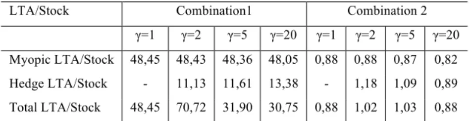
Table 6 – LTA and Foreign Asset to Brazilian Stock Ratios in Absolute Value
LTA/Stock Combination1 Combination 2
greater degree of predictability. It also tends to increase with the degree of persistence of state
variables that prove to be good predictors of these asset returns.
In combination 1, since LTA have a large positive Sharpe ratio, investors hold,
normally, long positions in these assets. Hence, an increase in expected LTA returns is
understood as an improvement in the investment opportunity set. According to our VAR
estimation, future LTA returns increase when the EMBI + spread increases (Table 3.1). Once
LTA are considerably negatively correlated with the EMBI + spread by 27,2%, poor LTA
returns are correlated with an improvement in future investment opportunities. Consequently,
conservative investors with 𝛾 > 1 can use LTA to hedge against the variation of their future
returns, resulting in a positive intertemporal hedging demand.
Stock returns also have a positive intertemporal hedging demand. First, the EMBI +
spread forecasts excess stock returns and LTA returns positively. Thus, an increase in the
stock return represents an improvement in the investment opportunity set. Since stock returns
are highly negatively correlated with changes in the risk of Brazil variable by -69,3%, this
generates a positive intertemporal hedging demand by conservative investors with 𝛾 > 1.
Still, there is a positive correlation between unexpected LTA returns and stock returns of
15,9%, so investors can offset their positive intertemporal hedging demand for LTA by taking
short positions in stocks. Although, the model yields a positive intertemporal hedging demand
for all levels of risk-aversion, meaning that the former effect more than compensates for the
later. Here, investors with 𝛾 > 1 have a positive total demand for stock, since intertemporal
hedging demand overweighs myopic demand. Strategic effects surpass tactical effects,
making it clear the importance of asset returns predictability in optimization.
Intertemporal hedging demand is smaller for stocks than for LTA, probably due to the
fact that LTA returns are more predictable than stock returns – LTA R-squared is the highest
In what concerns combination 2, following the same reasoning above, since the
Brazilian stock has a negative SR, investors hold, normally, short positions in these type of
assets. Hence, an increase in expected Brazilian stock returns is understood as a deterioration
in investment opportunities. Future Brazilian stock returns increase when the 12-month
accumulated dividend yield increases (Table 3.2). Once the Brazilian stock is considerably
positively correlated with the 12-month accumulated dividend yield by 11,4%, poor Brazilian
stock returns are correlated with an improvement in future investment opportunities.
Consequently, conservative investors with 𝛾 > 1 can use the Brazilian stock to hedge against
their future returns volatility, resulting in a negative intertemporal hedging demand.
Foreign stock returns also have a negative intertemporal hedging demand. There is a
negative correlation between unexpected Brazilian stock returns and foreign stock returns of
10,3%, so investors can offset their negative intertemporal hedging demand for Brazilian
stock by taking short positions in foreign stocks. The Brazilian Hedging stock to foreign
Hedging stock ratio is bigger than 1 for moderately conservative investors, probably due to
the former’s R-squared, which is higher than the foreign stock’s R-squared.
The same analysis of could have been made for combinations 3 and 4. There, LTA
returns are, once again, more predictable than stock returns, and intertemporal hedging
demand is bigger for LTA, than for stocks.
Figure 2.1 and Figure 2.2 plot the history of total and hedging asset allocations for 𝛾 =
5 and 𝜓 = 1 across the 3 assets of combination 1 and combination 2, respectively. Hedging
demands are less volatile than total demands for both combinations. Myopic allocations are
responsible for changing the sign of demands. Campbell et al. (2003) show that hedging demands only change sign in harsh events. Trying to follow such strategies is almost
Figure 2.1
Figure 2.2
5 Conclusion
We study the predictability of asset returns and its impact on long-term investors’
financial decisions. Intertemporal hedging demands are strategically relevant in optimal
portfolio allocation, contrary to myopic optimal allocations where they play a tactical role.
The state variables used to predict asset returns affect this demand for protection
through the correlation of their shocks to unexpected returns on stocks and long-term assets, -10000 -8000 -6000 -4000 -2000 0 2000 4000 6000 8000 10000 Ja n -06 Ju l-06 Ja n -07 Ju l-07 Ja n -08 Ju l-08 Ja n -09 Ju l-09 Ja n -10 Ju l-10 Ja n -11 Ju l-11 Ja n -12 Ju l-12 Ja n -13 Ju l-13 Ja n -14 Ju l-14 Ja n -15 Ju l-15 Ja n -16 Ju l-16
History of Asset Allocations - Combination 1
STA LTA Stock Hedging STA Hedging LTA Hedging Stock
-600 -400 -200 0 200 400 600 800 Ja n -06 Ju l-06 Ja n -07 Ju l-07 Ja n -08 Ju l-08 Ja n -09 Ju l-09 Ja n -10 Ju l-10 Ja n -11 Ju l-11 Ja n -12 Ju l-12 Ja n -13 Ju l-13 Ja n -14 Ju l-14 Ja n -15 Ju l-15 Ja n -16 Ju l-16
History of Asset Allocations - Combination 2
STA Foreign Stock Stock
and their persistence. Risk of Brazil, as measured by the EMBI + spread, and the 12-month
accumulated dividend yield has the highest correlations amongst all the state variables. These
state variables are the most important in defining the optimal portfolio demands.
We consider two types of asset combinations. First we use only Brazilian assets and
perform the predictability analysis. We innovate in combination 2 by replacing one of the
Brazilian components, the Long Term Assets (LTA), by a foreign index (the S&P500).
In the first combination, the long-term asset was the responsible for intertemporal
hedging demand. This demand arises from the high correlation between shocks to the variable
that help to predict returns, EMBI + spread, and shocks to long-term assets. We find that the
total optimal demand (strategic plus myopic) for long-term assets is positive. In this
combination, intertemporal hedging demand is positive, playing an important strategic role
for conservative investors, as opposed to the negative myopic allocation. Corroborating past
empirical research, we find that LTA returns are more predictable than stocks in Brazil, so
that intertemporal hedging demand is greater for LTA than for stocks.
Our analysis innovates by comparing investment in Brazilian assets with the
possibility of investing in a foreign index. In our set-up the foreign index is more predictable
for moderately conservative investors, than the Brazilian stocks. As a consequence,
moderately conservative investors use S&P 500 for intertemporal hedging.
This research is not free of limitations. Long-term investors have wealth, but labour
income is not modelled. Short-selling is not constrained. The results constitute an
approximation for investors with elasticity of intertemporal substitution different than one.
The VAR system is estimated without corrections for small-sample biases and Bayesian
priors were not used. Although, Banbura, Giannone, and Reichlin (2010) have shown that a
Bayesian vector auto regression model is more appropriate for modelling large data sets.
As the ANBIMA historical series will become longer, it will be worth to reassess the
demands for the assets with more robust estimates of the VAR parameters.
References
Banbura, T., Giannone, R., Reichlin, L., 2009. “Large Bayesian vector auto
regressions”. Journal of Applied Econometrics 25.
Barberis, N.C., 2000. “Investing for the long run when returns are predictable.” Journal of
Finance 55.
Campbell, J.Y., 1987. “Stock returns and the term structure.” Journal of Financial Economics
18.
Campbell, J.Y., 1991. “A variance decomposition for stock returns.” Economic Journal 101.
Campbell, J.Y., 1993. “Intertemporal asset pricing without consumption data.” American
Economic Review 83.
Campbell, J.Y., 1996. “Understanding risk and return.” Journal of Political Economy 104.
Campbell, J.Y., Chan, Y.L., Viceira, L.M., 2003. “A Multivariate Model of Strategic Asset
Allocation.” Journal of Financial Economics 67.
Campbell, J.Y., Viceira, L.M., 1999. “Consumption and portfolio decisions when expected
returns are time varying.” Quarterly Journal of Economics 114.
Campbell, J.Y., Viceira, L.M., 2000. “Consumption and portfolio decisions when expected
returns are time varying: erratum.” Unpublished paper, Harvard University.
Campbell, J.Y., Viceira, L.M., 2001. “Who should buy long-term bonds?” American
Economic Review 91.
Campbell, J.Y., Viceira, L.M., 2002, Strategic Asset Allocation, Oxford University Press. Epstein, L., Zin, S., 1989. “Substitution, risk aversion, and the temporal behavior of
consumption and asset returns: a theoretical framework.” Econometrica 57.
consumption and asset returns: an empirical investigation.” Journal of Political Economy 99.
Fama, E., French, K., 1989. “Business conditions and expected returns on stocks and bonds.”
Journal of Financial Economics 25.
Fama, E., Schwert, G., 1977. “Asset returns and inflation.” Journal of Financial Economics 5.
Giovannini, A., Weil, P., 1989. “Risk aversion and intertemporal substitution in the capital
asset pricing model.” NBER Working Paper 2824, Cambridge, MA.
Glosten, L.R., Jagannathan, R., Runkle, D., 1993. “On the relation between the expected
value and the volatility of the nominal excess return on stocks.” Journal of Finance 48.
Harvey, C., 1989. “Time-varying conditional covariances in tests of asset pricing models.”
Journal of Financial Economics 22.
Harvey, C., 1991. “The world price of covariance risk.” Journal of Finance 46.
Hodrick, R.J., 1992. “Dividend yields and expected stock returns: alternative procedures for
inference and measurement.” Review of Financial Studies 5.
Kandel, S., Stambaugh, R., 1987. “Long horizon returns and short horizon models.” CRSP
Working Paper 222, University of Chicago.
Markowitz, Harry. 1952. “Portfolio selection”. Journal of Finance 7.
Merton, R.C., 1969. “Lifetime portfolio selection under uncertainty: the continuous time
case.” Review of Economics and Statistics 51.
Merton, R.C., 1971. “Optimum consumption and portfolio rules in a continuous-time model.”
Journal of Economic Theory 3.
Samuelson, P.A., 1969. “Lifetime portfolio selection by dynamic stochastic programming.”
Review of Economics and Statistics 51.