Memory Storage Fidelity in the Hippocampal
Circuit: The Role of Subregions and Input
Statistics
Torsten Neher1,2*, Sen Cheng1,3, Laurenz Wiskott1,2
1International Graduate School Neuroscience, Ruhr-University Bochum, Bochum, Germany,2Institute for Neural Computation, Ruhr-University Bochum, Bochum, Germany,3Mercator Research Group‘Structure of Memory’, Department of Psychology, Ruhr-University Bochum, Bochum, Germany
Abstract
In the last decades a standard model regarding the function of the hippocampus in memory formation has been established and tested computationally. It has been argued that the CA3 region works as an auto-associative memory and that its recurrent fibers are the actual storing place of the memories. Furthermore, to work properly CA3 requires memory patterns that are mutually uncorrelated. It has been suggested that the dentate gyrus orthogonalizes the patterns before storage, a process known as pattern separation. In this study we review the model when random input patterns are presented for storage and investigate whether it is capable of storing patterns of more realistic entorhinal grid cell input. Surprisingly, we find that an auto-associative CA3 net is redundant for random inputs up to moderate noise levels and is only beneficial at high noise levels. When grid cell input is presented, auto-associa-tion is even harmful for memory performance at all levels. Furthermore, we find that Hebbian learning in the dentate gyrus does not support its function as a pattern separator. These findings challenge the standard framework and support an alternative view where the sim-pler EC-CA1-EC network is sufficient for memory storage.
Author Summary
It is well known that the hippocampus, a mammalian brain region, has a crucial role in memory formation. Furthermore, it has a remarkable anatomical structure and can be di-vided into several subregions based on physiological properties. Over the last decades a widely accepted model has evolved suggesting individual roles for each subregion in mem-ory storage. The central idea is that region CA3, with its remarkably many synapses that project into the region itself again, stores the memories within these synapses. In this model a memory is impressed onto the hippocampus by neuronal activation in the hippo-campal input region. Recently it has been found that such activations have a certain regu-larity instead of being random as assumed in the standard model. Here we investigate how well the model performs when storing memories of regular inputs. We find that the pro-posed function of CA3 actually harms memory performance. Moreover, we show that this
a11111
OPEN ACCESS
Citation:Neher T, Cheng S, Wiskott L (2015) Memory Storage Fidelity in the Hippocampal Circuit: The Role of Subregions and Input Statistics. PLoS Comput Biol 11(5): e1004250. doi:10.1371/journal. pcbi.1004250
Editor:Alessandro Treves, SISSA Intl Sch Adv Studies, ITALY
Received:September 22, 2014
Accepted:March 19, 2015
Published:May 8, 2015
Copyright:© 2015 Neher et al. This is an open access article distributed under the terms of the
Creative Commons Attribution License, which permits unrestricted use, distribution, and reproduction in any medium, provided the original author and source are credited.
Data Availability Statement:The computational code which we apply to create the data is available at:http://cns.mrg1.rub.de/index.php/software
function is redundant even in the case of random inputs. These findings call the standard model into question and support an alternative view of how the hippocampus may store memories.
Introduction
The crucial role of the hippocampus in memory formation is well known. Patients with damage to the hippocampus and its nearby cortices have severe deficits in acquiring new episodic mem-ory and in remembering events that happened shortly before the damage [1]. Impairments in memory formation can be observed in animals, too. For example, rats with a lesioned hippo-campus cannot associate stimuli if there is a time delay between them [2].
Furthermore, the hippocampus has a remarkable anatomical structure. Based on anatomical and physiological properties it can be divided into the dentate gyrus (DG) with its huge num-ber of small granule cells that show low activity [3] and the regions CA3 and CA1 consisting of a homogeneous set of pyramidal cells, where in CA3 one can find a striking number of recur-rent connections. A further notable property is that the connections among the subregions is established largely in a feedforward manner [4].
The question that arises is, how does this peculiar anatomical structure serve memory for-mation? Over the years, a standard framework has evolved regarding hippocampal functioning and it has been tested with a number of computational models (for example by Rolls (1995) [5]). The view is that the CA3 region functions as an auto-associative memory [6–9]. An auto-associative memory is a recurrent network that stores patterns in its feedback connections and can reconstruct these patterns when only a partial version of them is presented. Thus, the actu-al storing place are the recurrent connections and this idea could explain why there are so re-markably many in CA3.
An auto-associative memory can only store patterns that are not similar or mutually corre-lated [6]. By nature, however, the neural activation in the input region of the hippocampus, the entorhinal cortex (EC), is not uncorrelated [10]. Thus, it has been suggested that the DG per-forms pattern separation during the storage phase [7–9]. It decorrelates the patterns of the EC and projects the separated versions of the patterns to CA3 for storage. A large number of cells with low activity and the sparse projection of mossy fibers support pattern separation compu-tationally [11,12]. Hence, this view explains the appearance of yet other prominent hippocam-pal characteristics. Finally, it has been proposed that the role of CA1 is to decode the highly transformed patterns in CA3 back to their original versions in the EC.
A number of cells in the medial entorhinal cortex (MEC), called grid cells, fire at places in the environment regularly distributed on a hexagonal grid [10]. The present study reviews the model by Rolls and we test whether it is capable of storing grid cell input patterns. To our sur-prise, we find that CA3 functioning as an auto-associative memory is not only redundant, but harmful for memory performance. We even find a redundancy for random inputs at low to moderate noise levels. Moreover, pattern separation through the DG does not occur by simply applying Hebbian learning.
Since it was recently suggested that the subnetwork EC-CA1-EC already performs pattern completion [13], we tested whether this simpler network is indeed sufficient for
memory function.
Materials and Methods
Model Architecture and Activation Function
The model consists of the subregions entorhinal cortex (EC), dentate gyrus (DG), CA3 and CA1. Cell numbersNin each region and numbers of connections one cell in a downstream re-gion has with the upper rere-gion are summarized inFig 1. Cell numbers and numbers of connec-tions are derived from rat data [4,14] and scaled down by 100 and 10, respectively. Dividing the number of connections per cell by 100, too, would lead to CA3 cells that do not receive any input from the DG. On the other hand, leaving this number constant would result in triple con-nections among cell pairs in the network. Thus, we choose to scale by the square root of 100, which scales the total number of connections between two subregions by 100, too. Cells in our
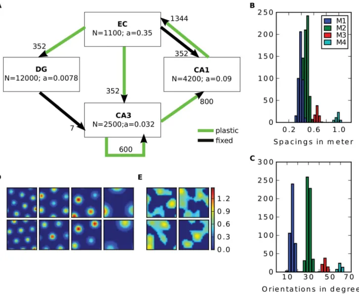
Fig 1. Model overview. A: The four subregions EC, DG, CA3 and CA1 are modeled.adenotes the proportion of cells being active at any given time. Arrows indicate connectivity among regions. Black ones are random and fixed connections, green ones are plastic and adjusted during learning. The number next to the arrows show the number of connections one cell in the downstream region has with the up stream region.B-C: Distribution of spacings (B) and
orientations (C) of the grid population in one environment. Colours indicate the modules.D-E: Four examples of grid cells (one from each module) (D) and two examples of LEC cells (E). The two rows show the firing map of the cells in two distinct environments.
model have continuous firing rates with the exception of CA3 cells, which are binary, i.e., they either fire and have the value 1 or are silent and have the value 0. This is in line with Rolls (1995), where CA3 does not work well with continuous firing rates [5].
A patternpof neural activation, for example,p2RNECþ in the EC triggers neural activity in
a downstream region, e.g., in the DG, via the connections as follows: First, the activationhiof
the output celliis calculated by the standard weighted sum of its inputs
hi ¼
XNEC
j¼1
wijpj; ð1Þ
wherewijis the strength of the connection from celljto celliand is defined as 0 whenever this
connection is not existent.
To determine the firing of a cell a simplek-Winner-Take-All (WTA) mechanism is applied: After calculating the activation of all cells of that region, thekcells with the highest activation are either set to 1 or tohiwhenever they are continuous. The others are inhibited and set to 0.
The numberkis determined by the sparsityaof that region, i.ek=aN. For instance, the pat-tern of neural activityq2RNDGþ in the DG is
qi ¼
(h
i if hi is among the k highest fhj: 1jNDGg
0 otherwise:
ð2Þ
Thus, inhibitory cells are not modeled explicitly but rather through their effect on a population level [15–19].
In order to determine the sparsityawe first estimated the average number of cells being ac-tive in one environment by referring to several studies that count acac-tive cells by immediate early genes [20–23] or by electrophysiological recordings [24,25]. Individual reports are sum-marized inTable 1and yield average activity levels of 2.9% in the DG, 22.7% in CA3 and 42.7% in CA1 across the enclosure. Second, for simplicity we assume that every active cell is a place cell and the proportion of the environment a place cell fires in is determined by its place field
Table 1. Overview of measured activity levels in hippocampal subregions.
Study Method Active cells %
DG
[23] (Fig 3) IEG 3
[22] (Fig 5) IEG 3–4
[21] (Fig 7) IEG 2.2
CA3
[20] (Fig 3c) IEG (Arc, Homer1) 18
[24] Electrophysiology 17–32
[25] Electrophysiology 26
CA1
[20] (Fig 3c) IEG (Arc, Homer1) 35
[24] Electrophysiology 48–66
[25] Electrophysiology 36
IEG means immediate early genes
size times the number of fields the cell has. Using data from recordings within a 1m2apparatus [24, Supplementary Table 1], we obtain an average coverage of 14% of a CA3 cell, and 21% of a CA1 cell. A typical DG cell has 3–4 fields and a field size smaller than 900cm2(personal com-munication with Edvard Moser) which brings us to an estimation of 27% coverage. Multiplying the proportion of cells being active across the environment by the proportion of the environ-ment one active cells fires leads to the activation level at one location given bya(seeFig 1). For the EC we calculated the average coverage of a grid cell to be 35% using data from Hafting et al. (2005) and assume that a grid cell is active in every environment [10,26]. This value is similar to the value obtained by the simulations from others [27].
Learning Rules
To store patterns in the network the plastic weights among subregions (green arrows inFig 1) are adjusted by three related Hebbian learning rules. LetCdenote the connection matrix of two regions, i.e.,cij= 1 if there is a connection from celljtoiandcij= 0 otherwise.
For the connections EC to CA3, CA3 to CA1, and CA1 to EC a rule for hetero-association is used. Let {p(s):1sM} be the set ofMinput patterns and {q(s):1sM} be the set of out-put patterns, then the connection strength is defined according to the so called Stent-Stinger rule [28]
wij¼cij
XM
s¼1
ðpðjsÞ pjÞq
ðsÞ
i ; ð3Þ
where the connection from celljtoiis the sum over all patternssoffiringpðjsÞof input cellj
subtracted by its meanp
jtimes thefiringq
ðsÞ
i of celli. The factorcijassures that non-existing
connections remain at zero weight.
For the synaptic weight matrixVof the recurrent weights in CA3 the co-variance rule is used [29] to learn an auto-association among a set of patterns {p(s):1sM}
vij¼cij
XM
s¼1
ðpðjsÞ pjÞðp
ðsÞ
i piÞ:
By subtracting the mean the two learning rules model LTP and LTD. Furthermore the subtrac-tion is essential for computasubtrac-tional reasons (see for example [30, chapter 8.2]).
Finally, the connections from EC to DG are altered by a one shot competitive learning rule. Here, the current input patternpfirst triggers a firing patternqin the downstream region ac-cording to the equations above. Synapses are then changed by
wij¼cijðwoldij þgpjqiÞ; ð4Þ
whereγis a constant learning rate. After applyingEq (4)the Euclidean norm of vectorwiof
After hetero-association of {p(s):1sM} with {q(s):1sM} by applyingEq (3) be-tween some regions, given patternp(t)as the present input we can rewrite the activationhðitÞas
hðitÞ ¼
XN
j¼1
wijp
ðtÞ
j
¼
ð3Þ XN
j¼1
cij
XM
s¼1
ðpðjsÞ pjÞq
ðsÞ
i p
ðtÞ
j
¼ qðitÞ
XN
j¼1
cijðp
ðtÞ
j pjÞp
ðtÞ
j þ
X
s6¼t
qðisÞ
XN
j¼1
cijðp
ðsÞ
j pjÞp
ðtÞ
j
qðitÞcðpðtÞ pÞ T
pðtÞ
|fflfflfflfflfflfflfflfflfflfflffl{zfflfflfflfflfflfflfflfflfflfflffl}
St
þX
s6¼t
c qðisÞðpðsÞ pÞ T
pðtÞ
|fflfflfflfflfflfflfflfflfflfflfflfflfflffl{zfflfflfflfflfflfflfflfflfflfflfflfflfflffl}
Xði;s;tÞ
;
wherecis the proportion of cells one output cell is connected to in the input layer. Thus, we can write the activation of cellias the sum of a signal termqiStwhich stems from the
propor-tion of the weights arising from the storage of patternp(t)and the crosstalk termsX(i,s,t)which
come from the contribution of the other stored patterns in which this cell was active [31]
hðitÞ q
ðtÞ
i Stþ
X
s6¼t
Xði;s;tÞ: ð5Þ
Ideally, the activation is high if and only if the cell hasfired in patternq(t).
Input
We perform simulations with random patterns and more realistic patterns that were generated by a grid cell code in the medial entorhinal cortex (MEC). For a randomly created pattern, cell activityhiis sampled from a normal distribution with mean and variance equal to 1. All cells,
but thekones with the highest activation are set to zero, as inEq (2). We store 252 patterns in both cases.
For the grid cell input we built a 1m by 1m virtual square environment. Each cell is
equipped with a hexagonal grid of place fields with equal size. The peak firing rate of each field is drawn from a uniform distribution from 0.5 to 1.5. According to the findings of Stensola et al. (2012) we divided the grid cell population into four modules [32]. Cells belonging to the same module have similar grid spacing and orientation. The cell parameter are drawn from normal distributions with variances 8 cm and 3 degree, respectively. The mean spacings of the modules are 38.8, 48.4, 65 and 98.4 cm and are taken from [32,Fig 1D]. The mean orientations are 15, 30, 45 and 60 degrees. The resulting distribution of spacings and orientations of the population is illustrated in Fig1B–1C. As in Stensola et al. (2012) there are more cells in the modules with small spacings.
Activation of celliat one location is determined by
hi¼e
d ri 2
logð5Þ
pðjiÞ;
wheredis the Euclidean distance to the nearestfield centerjandpðjiÞis the peak rate in that field andriis the radius. This way its activation isp
ðiÞ
j at the center and0:2p ðiÞ
j at the border of
400 locations are chosen randomly and the corresponding population activities were consid-ered as input patterns.
To study the influence of the lateral entorhinal cortex (LEC) we add input from LEC in some simulations. The activation map of one LEC cell is the summation of 30 place fields with random size at random locations. This is inspired by the findings of Deshmukh and Knierim (2011). They show that cells in the LEC tend to have several pseudo place fields that actually code for specific objects [33]. In Rennó-Costa (2010) LEC cells are modelled similarly. There, the cell’s activation map has specific active and non-active regions [15]. After defining the map in our model, we again set all LEC cells but thekones with the highest activation in each loca-tion to zero as inEq (2).
To study the effect of global remapping, input patterns from different environments are stored in some simulations. Here, each input cell has an activation map for each environment. For a grid cell, its activation map is computed by rotating and shifting its grid structure defined in the first environment, where the rotation angle and shifting vector is the same for the cells from the same module. This is inspired by the results of Fyhn et al. (2007), where they find a coherent remapping in cells recorded at the same location in the MEC [26]. For an LEC cell we define a completely new map for each environment in the same way as for the first map. Exam-ples of input cells and their remapping are shown in Fig1D–1E.
For recall a noisy version of a stored pattern is created, which we call recall cue. For each noisy pattern a subset of cells is selected randomly to fire incorrectly by setting its rate to that of an arbitrary other cell in that pattern. The quality of the cue is controlled by the number of cells that fire incorrectly and is measured by the Pearson correlation between original pattern and the recall cue.
Storage and Recall
Storing a patternpof entorhinal activation in the network is done as follows. First, this pattern triggers neural activity in the DG which in turn triggers a pattern in the CA3 region via Eqs (1) and (2). Thus, during storage, activity in CA3 is only influenced by the mossy fiber input from the DG. The connections from EC to DG are altered by the competitive learning rule (Eq (4)) for pattern separation. Hence, for the next pattern the connections are different as for the current pattern. Furthermore,pdrives an activity pattern in CA1. Now, the pattern in CA3 is hetero-as-sociated withpin EC, auto-associated in the recurrent connections in CA3, and hetero-associat-ed with the pattern in CA1. Finally, the CA1 activity is hetero-associathetero-associat-ed withpin the EC.
After the storage of all patterns the network is presented a recall cue by setting entorhinal activity to a noisy versionp^of a previously stored pattern. This activity triggers a patternq~ð0Þ
in CA3 directly via the previously learned weights from EC to CA3. The pattern then runs through 15 activation cycles of the auto-associative network in CA3 while leaving the input from the EC clamped (we have verified that after 15 cycles the results have converged). In more detail, for thet-th cycle the activation of CA3 celliis
hiðtÞ ¼a
XNEC
j¼1
wijp^þb
X
NCA3
j¼1
vijq~jðt 1Þ;
whereαandβare constant factors set to 1 and 3 andq~ðtÞis determined by the k-WTA
mecha-nism described inEq 2. Hence, during recall CA3 activity is dominated by the recurrent con-nections and the DG is not involved anymore. The resulting patternq~ð15Þtriggers one in
CA1, which in turn determines the output activity in the EC via the learned weights from CA3 to CA1 and CA1 to EC, respectively. In simulations without recurrent connectionsq~ð0Þ
Evaluation
Memory performance is determined by the network’s ability to perform pattern completion. In more detail, after storage, patterns are presented to the network again, but now in a corrupted version called recall cue. If the network’s output is more similar to the original pattern than its cue was, then the network has done some amount of recall. As a measure for similarity we use the Pearson correlation coefficient. For instance, the correlation between the originally stored patternpin the EC and the reconstructed onep~is defined as:
Corrðp;p~Þ ¼
ðp pÞTðp~ ~pÞ
kp pk kp~ p~k
;
wherepandp~are the means ofpandp~, respectively. The higher this correlation is, the more
similar is the recalled pattern to the original one. Furthermore, we define the average correla-tion over all stored patterns {p(s):1sM} as
CorrEC¼
1
M
XM
s¼1
CorrðpðsÞ;p~ ðsÞÞ
:
We perform simulations where we alter the quality of the recall cue and we illustrate the mem-ory performance by plottingCorrECover the quality of the cues, i.e. the average correlation the
cues have with the original patterns. Measurements above the main diagonal show then that the output of the network is on average more similar to the stored patterns than the cues. Hence, the more the measurements are above the diagonal, the better is the performance. To investigate how much pattern completion each subregion contributes to the overall perfor-mance, we similarly defineCorrCA3andCorrCA1.
Different Networks
We compare the model to two alternatives. Firstly, to determine how effective the CA3 recur-rent connections are, we perform simulations of a network without these connections. Here, the patternq~ð0Þis directly transferred to CA1 during recall without undergoing the activation
cycles of the auto-associative network in CA3. The result of these simulations are indicated by dashed lines throughout the figures.
Secondly, we investigate the ability of a minimal EC-CA1-EC model to store patterns. We performed simulations, in which during storage, activity in CA1 is triggered by the input from EC-CA3-CA1 pathway, without any plasticity in these connections. The CA1 patterns are then hetero-associated with the original input patterns in the connection weights EC-CA1 and CA1-EC, so in contrast to previous simulations the EC-CA1 connections are now plastic. Dur-ing the recall phase, the recall cue is transferred to CA1 via the temporoammonic pathway and from there back to EC. The result of these simulations are indicated by magenta lines through-out the figures.
Besides outlined architecture, parameters do not change across simulations except in section
‘Comparison to the Model in Rolls (1995)’. All parameter changes there are described in the main text.
Pattern Separation Index
good measure of how effective the DG separates the patterns. The flatter it is, the better is the separation. Thus, we refer to it as the pattern separation index.
Results
Comparison to the Model in Rolls (1995)
In a series of studies, a hippocampal model for memory formation within the standard frame-work has been established and tested computationally [5]. The main argument of this model is that CA3 equipped with many recurrent connections functions as an auto-associative network and is the crucial place for pattern completion. To test the theory, performance of simulations where those connections have been removed, has been compared to performance of the full network.
To reproduce the results of Rolls (1995) we performed a simulation of this model using the same parameters as in that study, including number of cells and connections and the sparse-ness parameter, and stored 100 random patterns.Fig 2Ashows the average correlation between stored patterns and the reconstructed ones in the EC vs. the cue quality. Since the curve is well above the diagonal the network as a whole performs pattern completion. Only when the cue quality becomes highly degraded, pattern completion starts to break down. The intermediate stages of the network, CA1 and CA3, while not as efficient as the entire network, perform pat-tern completion as well to a certain degree (Fig 2A). To specifically test the role of the recurrent connections in CA3, we performed the same analysis without those recurrent connections. In this case, pattern completion in CA3 was abolished (Fig 2A, dashed green line). However, as in the data of Rolls (1995), at the output level pattern completion was not affected. This has not been discussed and we will turn to this in more detail below. In conclusion, we reproduce the main results of the model (compareFig 2Awith [5,Fig 3bottom]).
While most of the parameters in the Rolls’model are consistent with the rat hippocampal anatomy, two clearly are not. Firstly, in the model CA1 the sparsity, i.e., the proportion of cells being active,aCA1= 1%, is much lower compared to the other regions, but the contrary is true
in the real rat hippocampus [24,34] (and see sparsity estimates inMethods). This way, many CA1 cells only code for one pattern as shown inFig 2Band the pattern a cell codes for is burned into the weights of that cell, which is reflected in a high learning rate in CA1. However, it is unrealistic to assume such a coding scheme. Since it allows CA1 to store only 1
aCA1¼ 100
patterns, even when numbers of cells and connections are scaled up to realistic ones of several hundreds of thousands as in the rat. This sparse coding scheme is functional, since the recall performance breaks down when we abandon it by increasing the sparsity to 10% (Fig 2C). In particular, patterns that are stored in the beginning of learning are overwritten by patterns that are stored later.
Secondly, full connectivity from CA1 to EC is assumed. This property is important, too. When the connectivity is diluted like between other regions, the low activity in CA1 is unable to trigger the whole original pattern in the EC (Fig 2D, diamonds). In this case, given a pattern in CA1, due to its high sparsity there are a few cells in EC that do not get any activation from it. However, this high connectivity is biologically not plausible.
Besides the changes in CA1, we scaled the model up and adjusted all parameters to more bi-ological plausible ones (Fig 1A) and simplified the activation function to a k-WTA mechanism (seeMethodsfor details). Overall, these changes did not alter the behaviour of the network (Fig 2E), although the presence of recurrence in CA3 now has a stronger effect on pattern comple-tion at the output stage. Notice also, that the complecomple-tion of the first hetero-associacomple-tion from EC to CA3 is much more effective. Due to a very sparse coding in Rolls’EC (5%) and a sparse connectivity the signal cannot be transferred properly to CA3 during recall. This is not the case in our model, since here the sparsity in EC is 35%.
From now on, all simulations are performed with continuous input, thus the model is now as described in the Method Section.
Fig 2. Analysis of the model by Rolls (1995). A: Recall performance in the model as proposed in [5]. Different colors show mean correlation between reconstructed patterns and stored ones in different regions; dashed lines show performance in a simulation where the recurrent connections in CA3 were turned off.B: Histogram of CA1 cell firing during storage. When sparsity is 0.01 (magenta) each cell fires about one time. This grandmother-like coding is abandoned if sparsity is 0.1 (black).C: Recall performance in CA1 (red) and EC (blue) for sparsity 0.1 measured for the last 10 patterns stored (stars) and for the first 10 (diamonds). Abandoning the grandmother-like code leads to a breakdown in performance by forgetting previously stored patterns.D: Recall performance in EC when connectivity from CA1 to EC is not complete and sparsity in CA1 is 0.01 (diamonds). A grandmother-like code cannot reproduce the whole pattern if the connectivity is sparse. When CA3-CA1 is a hetero-association with sparsity 0.1 (stars) diluting the connectivity has a milder effect.E: Our model as described in text yields similar results as inA, but is biologically more plausible, we believe.
Pattern Separation in DG
The standard framework suggests that the role of the DG is to perform pattern separation [7–9]. This process transforms correlated patterns in the EC into more uncorrelated ones in CA3. This is a necessary operation, since a Hopfield-like auto-associative memory in CA3 would only be efficient in storing patterns that are nearly orthogonal to each other [35]. [5] has suggested that pattern separation can be learned by a Hebbian competitive net, however, that has not been verified computationally. We therefore investigated whether DG is a good pattern separator and whether Hebbian learning enhances this function. We compared three different simulations. One with learning in the DG enabled, one where it is disabled, and one simulation, where we modeled the DG as a perfect pattern separator. In the last case, we removed the EC-DG-CA3 pathway and instead artificially set up a random uncorrelated code in CA3 for
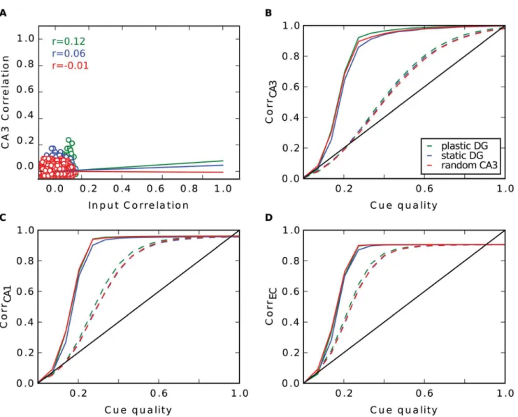
Fig 3. Pattern separation in the DG with random input. A: Pairwise correlation between stored patterns in CA3 as a function of pairwise correlation in EC with learning in DG (green), without (blue) and when the CA3 code is set up randomly (red). Regression lines are plotted, r values are shown in the upper left.
B-D: Recall performance of the different simulations in CA3 (B), CA1 (C) and EC (D). Dashed lines are simulations where the recurrent connections in CA3 have been removed.
storage. Each set of simulations were performed with random input and more realistic grid cell input (seeMethods).
As one might expect, with random input there are no great differences in performance be-tween the three simulations (Fig3B–3D). Patterns in the EC input are already uncorrelated by construction. This low degree of correlation is then just transferred to CA3. Hebbian learning in connections between EC and DG is not able to remove any more correlation (Fig 3A). Since the pairwise correlation in CA3 is not linearly dependent on the ones in EC (r value ranges from -0.01 to 0.12), the pattern separation index is not reliable here.
By contrast, with grid cell input from the EC, Hebbian learning has a strong effect on the network. One observation is the different firing behaviour of CA3 cells. Since each input tern refers to one location in space, we can illustrate the firing of CA3 cells over all stored pat-terns plotted over the environment (Fig 4A). Note that only 252 of the 400 locations can be occupied, as only 252 patterns were selected for storage. We observe that after learning, many cells in CA3 establish place fields. They fire around certain locations, but are silent elsewhere. This is in accordance to other work that have shown that Hebbian learning indeed transforms grid cell code into a place field representation [36–40]. Consequently, the probability a CA3 cell fires at locationsgiven it fires at locationtis significantly higher when the Euclidean dis-tance between these locations is small than when they are far away (green line inFig 4I). When learning is disabled, a typical cell in CA3 fires scattered over the entire space and is more com-parable to a CA3 cell that is created randomly, as in the third simulation. Hence, the probability it fires atsis no longer dependent on the distance totin the random CA3 case (red curve inFig 4I). This dependency is weaker when the DG connections are static (blue curve). In particular, the dependency extends to a smaller radius.
More interestingly, we find that Hebbian learning does not support pattern separation. To the contrary, we have measured the pairwise correlation between all stored patterns in CA3 and in EC and we have found that some patterns are highly similar in CA3 (Fig 4B) when learning is enabled. This is a direct consequence of the established place-field-like code in CA3. Patterns referring to close locations are very similar. Without learning, we do not see patterns of such high correlation, since CA3 cells are not as spatially selective as before. This is in line with the lower pattern separation index of the static DG (0.15) compared to the plastic one (0.28). In the simulation where the DG is modeled as a perfect separator the correlation be-tween two patterns is distributed around zero and no high correlations are found by definition.
In simulations without recurrent connections, the consequence of a place-field-like code in CA3 is a better recall performance in CA3 compared to the other scenarios, but a worse one at the output level in the EC (Fig4C–4E, dashed lines). To investigate the reason for the improve-ment in CA3 in this simulation, we looked at the activity distributions of cells during recall with a noiseless cue. We distinguished between activities of cells that should fire given the pres-ent recall cue and those of cells that should be silpres-ent. To no surprise, we find that the mean of the former is much higher. With plasticity in the DG the two distributions have very little over-lap (green curves inFig 4F). Thus, it is very rare that a cell that should be silent receives more activation than a cell that should be active. Hence, very few mistakes are made. In contrast, if the CA3 code is random, these distributions overlap more and false behaviour occurs more often.
What is the origin of this effect? InEq (5)we expressed the activation of celligiven the noiseless recall cuep(t)as the sum of the signalStand the crosstalk terms. In the random case,
the activations of cells that should be silent are distributed around 0. Here, in each activation the signal term vanishes (becauseqðitÞ ¼0) and it is only influenced by the sum of crosstalk
qðitÞ¼1) and the distribution is shifted to the right by the average signalS=hStitwhile its
shape is preserved (we find that the variance ofSis negligible). Hence, the sums of crosstalk terms are not dependent on whether a cell fired during storage or not.
In contrast, in a place-field-like code these distributions are not just shifted byS. Here, crosstalk terms tend to be larger, when a cell is supposed to fire (Fig 4G). Note that each cross-talk termX(i,s,t)is proportional toqðisÞ, the firing of celliat locations, times the overlap
ðpðsÞ pÞTpðtÞof the input pattern at locationswith the cue. Suppose cellihas fired att, as
seen inFig 4I,qðisÞis more likely to be non zero when locationsis nearby locationt.
Additional-ly, due the spatial character of the grid cell input, the overlap is highly dependent on the dis-tance, too, and is maximal when the locations are close by (Fig 4H). Thus, the more likely
qðisÞ¼1, the higher is the overlap as shown inFig 4J(green dots). This is not true when celli
has been silent att(Fig 4K). Here, the cell is less likely to fire at nearby locations and hence crosstalk terms with a large overlap factor do vanish at least as often as others. Therefore, cross-talks are greater in cells that should be active than in cells that should not. This explains the higher activation of cells that should be active and the better performance.
When learning is disabled the probability ofqðisÞis less dependent on the distance ofsandt.
Hence, the relation of the overlap withqðisÞis less pronounced (blue dots inFig 4J).
Consequent-ly, this relation disappears in a random CA3 code, since here a CA3 cell fires entirely indepen-dently on the distance (red dots inFig 4J).
The advantage in performance when learning is enabled, however, is already gone at the CA1 stage (dashed lines inFig 4D). Due to the high similarity of some patterns in CA3, some crosstalk terms in CA1 become very large. The consequence is a high variance of the sum of crosstalks and hence wider distributions of activities of cells that should be active and of those that should not. This results in a high overlap between these two distributions, thus many er-rors are made (Fig 4L).
Without Hebbian learning in the DG and in the simulation where the DG is a perfect sepa-rator, we do not see this high variance because of the lack of patterns that are highly similar. Here, the distributions are sharper resulting in less overlap and fewer mistakes (Fig 4L).
Furthermore, the recall correlations in CA3 without recurrent connections are very low, in particular when the CA3 patterns are created randomly (red dashed line inFig 4C). This re-quires an explanation.
Even though the 252 patterns stored in CA3 are orthogonal and span a high dimensional space, due to the high correlations in the grid input, the learned EC-CA3 weights, span a much lower dimensional space. When CA3 patterns are projected into this low-dimensional sub-space, the correlation between recalled and stored patterns are high, i.e., the EC-CA3 hetero-as-sociation works in principle. However, when assessing the retrieval quality, we compare the retrieved to the stored pattern in the larger dimensional space of CA3 patterns. Since the EC-CA3 weights span a low-dimensional space, they cannot address the higher dimensional space and, therefore, the correlations between stored and recalled patterns are low, and the dashed red line inFig 4Cis far below the diagonal.
and are silent during storage (dashed).H: Average overlap of two pattensp(s)
andp(t)
in the EC plotted over the distance ofsandt.I: Probability that a CA3 cell fires at a location s given it fires at t plotted over the Euclidean distance of s and t. Inset shows zoomed plot.J: Average Overlap of two pattensp(s)and p(t)in the EC plotted over the probability a cell fires atsgiven it fires att.K: Probability a cell fires at s, given it is silent at t. Inset shows zoomed plot.L: Same asFbut in CA1.
The recurrent collaterals in CA3 are doing their job well in the random CA3 case since the solid red line is well above the dashed one inFig 4C. However, the solid red line is still barely above the diagonal for low to moderate cue quality and well below for high cue quality, because the auto-associative net cannot entirely overcome the limitation of the EC-CA3 projections. As in the network without recurrent connections, when patterns are projected onto the low-di-mensional subspace, recall performance would be much better. That information about the stored input patterns is preserved in CA3, despite the low retrieval correlations, is evident when examining the later stages of hippocampal processing, in CA1 (Fig 4D) and EC output (Fig 4E). There, the retrieval performance is quite high for random CA3 patterns. The fact that it is better than for the static or plastic DG case confirms that auto-associative networks per-form best for uncorrelated (CA3) patterns.
For the static and plastic DG case, we find that without recurrent connections performance is better than for random CA3 patterns (Fig 4C, green and blue dashed lines lie above red dashed line) and that the difference between recurrent and no recurrent connections is less pronounced (compare respective solid to dashed lines). These findings lend further support to our explanation for the retrieval correlations for random CA3 patterns. When DG is static or plastic, the pattern in CA3 is driven to a certain extend by the EC input (via DG) and thus is correlated with it. Therefore, the mismatch between the dimensionality of the CA3 patterns and that of the EC inputs is lower and, as a result, the retrieval correlations in CA3 are higher. However, the correlations between stored CA3 patterns reduce the ability of the CA3 recurrent network to perform pattern completion, which hurts retrieval performance in the downstream layers (Fig4Dand4E).
To summarize, Hebbian plasticity does not enhance pattern separation as suggested in [5]. When grid input is given, it has even the contrary effect and hence harms memory perfor-mance. Moreover, we find that a static DG performs decent pattern separation. Therefore, in the following analysis learning in the DG is disabled.
Pattern Completion in CA3
To test the hypothesis that CA3 functions as an auto-associative memory, we compared a sim-ulation of the complete network with one, where we disabled the recurrent connections. Once again, we perform this comparison for random and grid cell inputs.
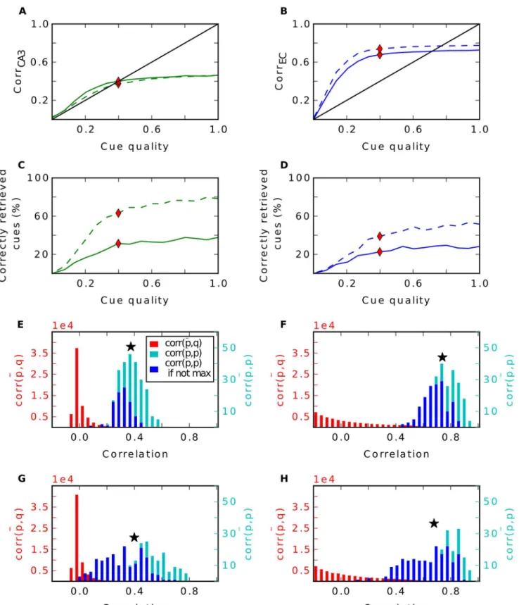
When random inputs are presented, we indeed find the recurrent connections performing a fair amount of pattern completion in CA3 (Fig 5A) as also found by [5]. At the output stage in the EC, however, the recurrent connections in CA3 are only beneficial when cues are highly de-graded. Both simulations with and without recurrent CA3 connections perform equally well for strong to moderate cue qualities (Fig 5B). Thus, in these cases the hetero-associative steps EC-CA3, CA3-CA1 and CA1-EC are already sufficient for pattern completion.
In more detail, the mean of the distribution of correlations between the reconstructed pat-terns and their original version is increased by the recurrent connections, which is good. How-ever, at the same time, this distribution becomes wider and even bimodal. Thus, it begins to intersect with the distribution of correlations between the reconstructed patterns and all other stored pattern. Consequently, it starts to confuse reconstructed patterns with the other stored ones (Fig 5G). This confusion cannot be solved at later stages and the correlation between these patterns and their originals stays low till the output stage (Fig 5H). The result is a bimodal distribution of correctly remembered patterns with high correlation and false recalled ones with correlation around 0. When the recurrent connections are disabled, the distribution of correlations in the EC stays unimodal with a lower mean but fewer patterns are confused (Fig 5F).
To summarize, for moderate to good cue qualities, the computation of the recurrent con-nections is completely redundant, since the pattern completion is also performed by the inevi-table decoding pathway over CA1. For weak cues, the recurrent connections do help recall, but this advantage comes at the price of a higher confusion rate.
We also tested how effective the pattern completion by the recurrent connections is in the grid cell input scenario. We observe that having these connections helps in CA3 only marginal-ly, but at the price of a significantly higher confusion rate (Fig6A–6H). More importantly, at the output level in EC the recurrent connections become a deficiency for the model and the performance is worse. Additionally, the higher confusion rate is still apparent. Thus, the recur-rent connections are not only redundant but even harmful for memory performance for all cue qualities.
Recall by the EC-CA1-EC Pathway
An alternative proposal is that pattern completion is performed by the pathway EC-CA1-EC [13]. Our data shows that recurrence in CA3 is redundant and that three hetero-associations are sufficient for completion. We investigated, whether the two associations EC-CA1-EC are sufficient for pattern completion as well. The results are shown inFig 7.
When input patterns are created randomly, the simpler model confuses fewer patterns (Fig
7C–7D), but performance in terms of correlation is worse than with the complete network (Fig
7A–7B). It seems that in this scenario two steps are not sufficient to reconstruct the whole pat-tern. Interestingly, in the more realistic grid cell input scenario, the two steps in the alternative model are slightly more effective in pattern completion than the complete network (Fig7E– 7F). Moreover, the former confuses far fewer patterns than the latter (Fig7G–7H).
We wondered whether scaling factors effect the model. Thus, we performed simulations as inFig 7where we scaled down the number of neurons by only 20 rather than by 100. We stored 2525 patterns while leaving all other parameters constant. In particular, the number of synap-ses is still scaled by 10. We find no qualitative differences between the simulations indicating that our results do not change when numbers of cells and synapses approach the realistic ones.
reconstructed pattern and another stored pattern (red). Blue indicate the cases when the correlation between the reconstructed pattern and the stored pattern is not maximal. Star marks mean of the distribution of the correlation between the reconstructed pattern and the stored pattern. The histogram is calculated at the cue quality indicated by the red rhombus inA-D.G-H: Same asE-Fbut with recurrent connections enabled.
Fig 7. Comparison of the complete model with the simpler EC-CA1-EC model.Performance of the complete model (green and blue) and of the simpler EC-CA1-EC model (magenta) when random input is given (A-D) and grid input is given (E-H).A: Recall performance in CA3 (complete model) and CA1 (simpler model).B: Performance in EC.C-D: Proportion of correctly retrieved patterns in CA3/CA1 (C) and EC (D), respectively; dashed lines are simulations without recurrent connections.E-H: Same as left column, but with grid cell input.
LEC Input and Different Environments
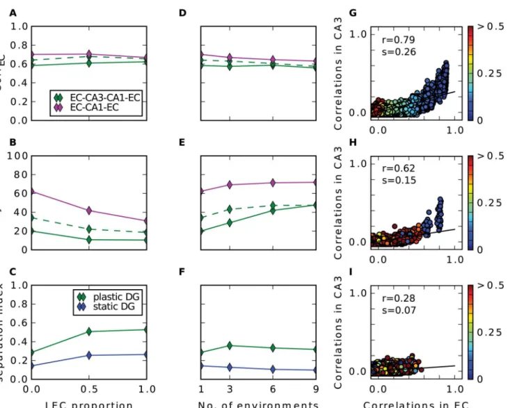
Up to now we have considered only input to the hippocampus that originates from the medial part of the entorhinal cortex. Studies have shown that substantial part of hippocampal input comes from the lateral entorhinal cortex (LEC). In contrary to the grid cells, neurons in LEC fire only weakly spatially modulated [41] and rather respond to individual objects [33]. How do the networks behave under the influence of such input? Since the proportion of LEC input relative to MEC input is not clear, we parametrized it and performed simulations with different proportions of LEC cells. We find that the recall correlations in EC are not affected much by adding LEC input (Fig 8A). When input comes only from LEC the networks confuse patterns more often. Because of the pseudo place field code in LEC, nearby patterns are highly
Fig 8. LEC input and multiple environments.Results of simulations with additional LEC input (A-C) and with input from multiple environments (D-F). First row (A, D) shows the recall correlation in EC averaged over all cue strengths, second row (B, E) shows averaged proportion of correctly retrieved patterns and last row (C, F) shows pattern separation index.G: Pairwise correlation between stored patterns in CA3 as a function of pairwise correlation in EC in a simulation with only LEC inputs. Euclidean distance (in m) of the pair is indicated by the colour of disk according to the colourbar. Black line is the regression line with slope s (separation index) and r value shown in the upper left.H-I: Same as (G) in a simulation with only MEC input originating from nine different environments.Hshows all pairs where both patterns come from the same map,Ishow all pairs where the patterns come from different maps.
correlated and the radius to which this extends is slightly larger than in the grid cell code (com-pareFig 8GwithFig 4B). Consequently, the number of high correlated patterns is higher which results in a higher confusion as well as in a slightly less effective pattern separation.
Fyhn et al. (2007) found that when a rat is exposed to a new environment the grid cells remap, i.e. their grid pattern rotates and shifts coherently while the spatial frequency remains roughly stable [26]. We investigated how well the networks can store patterns of activity origi-nating from different environments rather than from just one. We find that by increasing the number of maps, the recall correlations and the proportion of correctly retrieved patterns of the networks with and without recurrent connections become almost equal, where the EC-CA1-EC network remains the best in both measures (Fig8D–8E).
As argued above, already a small number of moderately correlated patterns in CA3 degrades the auto-association and the subsequent hetero-association with CA1. Given just one map, cor-relation appears only in patterns that are nearby. We wondered, whether this is still true com-paring patterns from different environments. In Fig8H–8Iwe see the pairwise correlations of stored patterns in CA3 over the ones in the input in a simulation where we store patterns from nine different environments. Comparing patterns that originate from the same map, only those that are up to 5 cm apart have a high correlation above 0.6 and these are the only pairs, that remain to have moderate correlations left in CA3(Fig 8H). Many pairs, that are not nearby, have a fair correlation in the input but are almost uncorrelated after pattern separation through the DG. This can be observed for pairs where each pattern is from a different environment, too (Fig 8I). Many of them are moderately correlated in the input, but no longer in CA3. The re-mapping of the grids does not orthogonalizes the activities in the EC. Nevertheless, after pat-tern separation by the DG the patpat-terns become almost uncorrelated in CA3.
To conclude, when patterns are stored from several environments, the relative number of pattern pairs that are nearby and from the same environment decreases and with it the number of pairs with remaining correlation in CA3. This benefits in particular the recurrent network and it performs as well as the network without recurrent connections. Nevertheless, the EC-CA1-EC network performance is best in all scenarios.
Discussion
In the last decades, a view has evolved about how the peculiar anatomic structure of the hippo-campus serves memory formation. It has been postulated that the CA3 region with its many re-current connections functions as an attractor network performing pattern completion when degraded input is given [7,11]. Thus, it is believed that CA3 is the actual storing place. Com-plex mathematical analysis show that the memory capacity of such a network is sufficient, when the activity in the region is sparse enough [30,35,42]. However, a decorrelation among the stored patterns is crucial and all the analysis supposes that. It is believed that the DG re-moves all correlations from the input patterns of the EC and performs the so called pattern sep-aration. This is supported by a sparse coding, by strong and sparse synapses from DG to CA3 [9,11], and by Hebbian plasticity from EC to DG during storage [5].
the activity approaches zero, the performance of a single auto-associative memory reaches nearly that of several hetero-associations, while at the same time fewer neuronal components are needed. However, in the standard model these components have to be present to perform encoding and decoding, turning this argument against the proposed function of CA3.
Secondly, simple Hebbian plasticity in the DG as proposed by Rolls (1995) does not support pattern separation. To the contrary. We have shown that due to this plasticity the grid cell code in the EC is mapped into a place field like code in CA3. This is in line with other work, that in-vestigate the transformation from grid cells to place cells [36–40] by Hebbian learning. In this code, patterns from nearby locations happen to be highly correlated, which is the opposite of what a pattern separator should do. Thus, a competitive net is not a good candidate to orthogo-nalize patterns for grid cell input. What is not modeled here, is adult neurogenesis in the DG [43]. This additional plasticity might support pattern separation in contrast to Hebbian learn-ing alone. Weisz and Argibay (2009) studied the effects of neurogenesis in the standard model and they find advantages in memory performance, but they only considered the case of random inputs [44]. However, alternative hypotheses for adult neurogenesis exist (e.g [18]). We show that by having random and fixed connections the DG performs quite well as a pattern separa-tor. Only for very highly correlated patterns in the input, there remains some amount of corre-lation in these patterns after applying the separator. Despite the significant reduction, this amount is still enough to degrade the auto-associative CA3. Thus, to make the standard model work, a separator is needed that functions perfectly. However, assuming it exists, the benefit of a recurrent CA3 net would still be small compared to the EC-CA1-EC model if applied to grid cell input.
Thirdly, a further challenging argument against an auto-associative function of CA3 is the fact that the actual representations in the mammalian CA3 are far from uncorrelated. The vast majority of active pyramidal cells are place cells [45], thus activity patterns are correlated by na-ture. Storing such patterns of continuous place cell activity that occur in one environment in an auto-associative network leads to a continuous attractor or so called chart [46]. Every point in this chart refers to the neural representation of one location in the environment. A degraded input is then attracted towards a point on the chart and the network is indeed able to diminish the noise orthogonal to the attractor. However, it has been observed that many points are not stable [47] and drift along the attractor until they reach a fix point [48]. This means that many finally retrieved patterns are representations of the wrong location. Since we store correlated patterns in the auto-associative CA3 net, a continuous attractor is also formed in the present model. It can store a large number of patterns drawn from the grid map moderately well, how-ever, drifting occurs in the recall. This drifting is already reduced, since the CA3 representa-tions are binary rather than continuous [49], but still apparent as reflected by the high confusion rate of patterns when using the recurrent connections in CA3 (seeFig 6C). Papp et al.(2007) state that the drift may be much slower than pattern completion and hence storage of locations is still possible [49]. In other words, pattern completion is already done in the first update cycles in the attractor network. This is in agreement with our results. By viewing each hetero-associative step as one update cycle, pattern completion is performed by the three asso-ciative networks without loosing accuracy caused by the drift and the auto-assoasso-ciative function in CA3 becomes redundant.
problems. A further alternative to an attractor net in CA3 has been suggested by Cheng (2013). Here, it is assumed that the recurrent CA3 network is not plastic, but rather creates intrinsic se-quences which are then associated with temporal sese-quences of patterns in the EC [13]. We do not model temporal aspects here, but our study shows that because of the redundancy of CA3 as an auto-associative net, it very likely fulfils some other function. Similarly, the minimal model does not require plasticity in the synapses projecting from EC to CA3 nor in the Schaffer Collaterals, where plasticity has been found [51]. Hence, the plasticity could serve another function leaving the pattern completion in the model unaffected.
Experimental studies reported evidence for CA3 being an auto-association memory. For ex-ample, Gold and Kesner (2005) show that rats with lesioned CA3 are impaired in remembering a location when parts of the spatial cues are removed [52]. Another study obtains similar re-sults when plasticity in CA3 synapses is corrupted in knock-out mice [53]. The authors con-clude that CA3 is crucial for spatial pattern completion. In our opinion this is not convincing. If the actual storing place of the memory is CA3 then lesioning it or removing plasticity should give equivalent results as lesioning the entire hippocampus [13]. This is not the case, since in both studies animals behave normally in full cue conditions, but animals with hippocampal le-sions are clearly impaired [54,55]. An alternative interpretation for the experimental observa-tions could be that the animals rely more on the integration of self motion cues in condiobserva-tions when external cues are poor. This is in line with others who assign a path integration function to CA3 [46,56]. If spatial information provided by the external cues is sufficient, spatial recog-nition can be performed by CA1 alone [57,58].
Our work illustrates how essential it is to consider the whole hippocampal loop while inves-tigating individual functional roles of the subregions.
Author Contributions
Conceived and designed the experiments: TN SC LW. Performed the experiments: TN. Ana-lyzed the data: TN SC LW. Contributed reagents/materials/analysis tools: TN. Wrote the paper: TN SC LW.
References
1. Milner B, Corkin S, Teuber J (1968) Further analysis of the hippocampal amnesic syndrome: A 14-year follow-up study of HM. Neuropsychologia 6: 215–234. doi:10.1016/0028-3932(68)90021-3
2. Gluck MA, Myers CE (2001) Gateway to memory. Cambridge, MA, USA: MIT Press.
3. Leutgeb JK, Leutgeb S, Moser MB, Moser EI (2007) Pattern separation in the dentate gyrus and CA3 of the hippocampus. Science 315: 961–966. doi:10.1126/science.1135801PMID:17303747
4. Amaral DG, Ishizuka N, Claiborne BJ (1990) Neurons, numbers and the hippocampal network. Prog-ress in Brain Research 83: 1–11. doi:10.1016/S0079-6123(08)61237-6PMID:2203093
5. Rolls ET (1995) A model of the operation of the hippocampus and enthorhinal cortex in memory. Inter-national Journal of Neural Systems 6: 51–70.
6. Marr D (1971) Simple memory: a theory for archicortex. Philosophical Transactions of the Royal Society of London, Series B 262: 23–81. doi:10.1098/rstb.1971.0078
7. McNaughton BL, Morris RGM (1987) Hippocampal synaptic enhancement and information storage within a distributed memory system. Trends in Neurosciences 10: 408–415. doi:10.1016/0166-2236 (87)90011-7
8. Treves A, Rolls ET (1994) Computational analysis of the role of the hippocampus in memory. Hippo-campus 4: 374–391. doi:10.1002/hipo.450040319PMID:7842058
9. O’Reilly RC, McClelland JL (1994) Hippocampal conjunctive encoding, storage, and recall: avoiding a trade-off. Hippocampus 4: 661–682. doi:10.1002/hipo.450040605PMID:7704110
11. Rolls ET (2007) An attractor network in the hippocampus: Theory and neurophysiology. Learning & Memory 14: 714–731. doi:10.1101/lm.631207
12. Treves A, Tashiro A, Witter MP, Moser EI (2008) What is the mammalian dentate gyrus good for? Neu-roscience 154: 1155–1172. doi:10.1016/j.neuroscience.2008.04.073PMID:18554812
13. Cheng S (2013) The CRISP theory of hippocampal function in episodic memory. Frontiers in Neural Cir-cuits 7: 88. doi:10.3389/fncir.2013.00088PMID:23653597
14. Vassilis C, Bruce G, Stuart C, Imre V (2010) Hippocampal Microcircuits. A Computational Modeler’s Resource. Springer New York.
15. Rennó-Costa C, Lisman J, Verschure P (2010) The mechanism of rate remapping in the dentate gyrus. Neuron 68: 1051–1058. doi:10.1016/j.neuron.2010.11.024PMID:21172608
16. Roudi Y, Treves A (2008) Representing where along with what information in a model of a cortical patch. PLoS Comput Biol 4. doi:10.1371/journal.pcbi.1000012PMID:18369416
17. Moustafa AA, Myers CE, Gluck MA (2009) A neurocomputational model of classical conditioning phe-nomena: A putative role for the hippocampal region in associative learning. Brain Research 1276: 180–195. doi:10.1016/j.brainres.2009.04.020PMID:19379717
18. Appleby PA, Kempermann G, Wiskott L (2011) The role of additive neurogenesis and synaptic plasticity in a hippocampal memory model with grid-cell like input. PLoS Comput Biol 7: e1001063. doi:10.1371/ journal.pcbi.1001063PMID:21298080
19. Monaco J, Abbott L (2011) Modular realignment of entorhinal grid cell activity as a basis for hippocam-pal remapping. Journal of Neuroscience 31: 9414–9425. doi:10.1523/JNEUROSCI.1433-11.2011 PMID:21697391
20. Vazdarjanova A, Guzowski JF (2004) Differences in hippocampal neuronal population responses to modifications of an environmental context: Evidence for distinct, yet complementary, functions of CA3 and CA1 ensembles. The Journal of Neuroscience 24: 6489–6496. doi: 10.1523/JNEUROSCI.0350-04.2004PMID:15269259
21. Alme CB, Buzzetti RA, Marrone DF, Leutgeb JK, Chawla MK, et al. (2010) Hippocampal granule cells opt for early retirement. Hippocampus 20: 1109–1123. doi:10.1002/hipo.20810PMID:20872737
22. Marrone DF, Adams AA, Satvat E (2011) Increased pattern separation in the aged fascia dentata. Neu-robiology of Aging 32: 2317.e23. doi:10.1016/j.neurobiolaging.2010.03.021
23. Satvat E, Schmidt B, Argraves M, Marrone DF, Markus EJ (2011) Changes in task demands alter the pattern of zif268 expression in the dentate gyrus. The Journal of Neuroscience 31: 7163–7167. doi:10. 1523/JNEUROSCI.0094-11.2011PMID:21562279
24. Leutgeb S, Leutgeb JK, Treves A, Moser MB, Moser EI (2004) Distinct ensemble codes in hippocampal areas CA3 and CA1. Science 305: 1295–1298. doi:10.1126/science.1100265PMID:15272123
25. Lee I, Yoganarasimha D, Rao G, Knierim JJ (2004) Comparison of population coherence of place cells in hippocampal subfields CA1 and CA3. Nature 430: 456–459. doi:10.1038/nature02739PMID: 15229614
26. Fyhn M, Hafting T, Treves A, Moser MB, Moser EI (2007) Hippocampal remapping and grid realignment in entorhinal cortex. Nature 466: 190–194. doi:10.1038/nature05601
27. de Almeida L, Idiart M, Lisman JE (2009) The input–output transformation of the hippocampal granule cells: From grid cells to place fields. The Journal of Neuroscience 29: 7504–7512. doi:10.1523/ JNEUROSCI.6048-08.2009PMID:19515918
28. Stent GS (1973) A physiological mechanism for Hebb’s postulate of learning. Proceedings of the Na-tional Academy of Sciences 70: 997–1001. doi:10.1073/pnas.70.4.997
29. Sejnowski TJ (1977) Storing covariance with nonlinearly interacting neurons. Journal of Mathematical Biology 4: 303–321. doi:10.1007/BF00275079PMID:925522
30. Amit DJ (1989) Modeling Brain Function: The World of Attractor Neural Networks. Cambridge, UK: Cambridge University Press.
31. Willshaw D, Dayan P (1990) Optimal plasticity from matrix memories: What goes up must come down. Neural Comput 2: 85–93. doi:10.1162/neco.1990.2.1.85
32. Stensola H, Stensola T, Solstad T, Froland K, Moser MB, et al. (2012) The entorhinal grid map is discre-tized. Nature 492: 72–78. doi:10.1038/nature11649PMID:23222610
33. Deshmukh SS, Knierim JJ (2011) Representation of nonspatial and spatial information in the lateral en-torhinal cortex. Frontiers in Behavioral Neuroscience 5. doi:10.3389/fnbeh.2011.00069PMID: 22065409
35. Hopfield JJ (1982) Neural networks and physical systems with emergent collective computational abili-ties. Proceedings of the National Academy of Sciences of the United States of America 79: 2554– 2558. doi:10.1073/pnas.79.8.2554PMID:6953413
36. Rolls ET, Stringer SM, Elliot T (2006) Entorhinal cortex grid cells can map to hippocampal place cells by competitive learning. Network 17: 447–465. doi:10.1080/09548980601064846PMID:17162463
37. Franzius M, Vollgraf R, Wiskott L (2007) From grids to places. Journal Computational Neuroscience 22: 297–299. doi:10.1007/s10827-006-0013-7
38. Si B, Treves A (2009) The role of competitive learning in the generation of DG fields from EC inputs. Cognitive Neurodynamics 3: 177–187. doi:10.1007/s11571-009-9079-zPMID:19301148
39. Savelli F, Knierim JJ (2010) Hebbian analysis of the transformation of medial entorhinal grid-cell inputs to hippocampal place fields. Journal of Neurophysiology 103: 3167–3183. doi:10.1152/jn.00932.2009 PMID:20357069
40. Cheng S, Frank LM (2011) The structure of networks that produce the transformation from grid cells to place cells. Neuroscience 197: 293–306. doi:10.1016/j.neuroscience.2011.09.002PMID:21963867
41. Hargreaves EL, Rao G, Lee I, Knierim JJ (2005) Major dissociation between medial and lateral entorhi-nal input to dorsal hippocampus. Science 308: 1792–4. doi:10.1126/science.1110449PMID: 15961670
42. Treves A, Rolls ET (1991) What determines the capacity of autoassociative memories in the brain? Net-work: Computation in Neural Systems 2: 371–397. doi:10.1088/0954-898X/2/4/004
43. Gross CG (2000) Neurogenesis in the adult brain: death of a dogma. Nature Reviews Neuroscience 1: 67–73. doi:10.1038/35036235PMID:11252770
44. Weisz VI, Argibay PF (2009) A putative role for neurogenesis in neurocomputational terms: Inferences from a hippocampal model. Cognition 112: 229–240. doi:10.1016/j.cognition.2009.05.001PMID: 19481201
45. O’Keefe J (1976) Place units in the hippocampus of the freely moving rat. Experimental Neurology 51: 78–109. doi:10.1016/0014-4886(76)90055-8PMID:1261644
46. Samsonovich A, McNaughton BL (1997) Path integration and cognitive mapping in a continuous at-tractor neural network model. The Journal of Neuroscience 17: 5900–5920. PMID:9221787
47. Tsodyks M, Sejnowski T (1995) Associative memory and hippocampal place cells. International Journal of Neural Systems 6: 81–86.
48. Cerasti E, Treves A (2013) The spatial representations acquired in CA3 by self-organizing recurrent connections. Frontiers in Cellular Neuroscience 7: 112. doi:10.3389/fncel.2013.00112PMID: 23882184
49. Papp G, Witter MP, Treves A (2007) The CA3 network as a memory store for spatial representations. Learning & Memory 14: 732–744. doi:10.1101/lm.687407
50. Levy WB (1996) A sequence predicting CA3 is a flexible associator that learns and uses context to solve hippocampal-like tasks. Hippocampus 6: 579–590. doi:10.1002/(SICI)1098-1063(1996)6:6% 3C579::AID-HIPO3%3E3.0.CO;2-CPMID:9034847
51. Buchanan K, Mellor J (2010) The activity requirements for spike timing-dependent plasticity in the hip-pocampus. Frontiers in Synaptic Neuroscience 296: 2243–2246.
52. Gold AE, Kesner RP (2005) The role of the CA3 subregion of the dorsal hippocampus in spatial pattern completion in the rat. Hippocampus 15: 808–814. doi:10.1002/hipo.20103PMID:16010664
53. Nakazawa K, Quirk MC, Chitwood RA, Watanabe M, Yeckel MF, et al. (2002) Requirement for hippo-campal CA3 NMDA receptors in associative memory recall. Science 297: 211–218. doi:10.1126/ science.1071795PMID:12040087
54. Morris RG, Garrud P, Rawlins JN, O’Keefe J (1982) Place navigation impaired in rats with hippocampal lesions. Nature 297: 681–683. doi:10.1038/297681a0PMID:7088155
55. Gilbert PE, Kesner RP, DeCoteau WE (1998) Memory for spatial location: role of the hippocampus in mediating spatial pattern separation. The Journal of Neurosciences 18: 804–810.
56. Colgin LL, Leutgeb S, Jezek K, Leutgeb JK, Moser EI, et al. (2010) Attractor-map versus autoassocia-tion based attractor dynamics in the hippocampal network. Journal of Neurophysiology 104: 35–50. doi:10.1152/jn.00202.2010PMID:20445029
57. Brun VH, Otnass MK, Molden S, Steffenach HA, Witter MP, et al. (2002) Place cells and place recogni-tion maintained by direct entorhinal-hippocampal circuitry. Science 296: 2243–2246. doi:10.1126/ science.1071089PMID:12077421

![Fig 2. Analysis of the model by Rolls (1995). A: Recall performance in the model as proposed in [5]](https://thumb-eu.123doks.com/thumbv2/123dok_br/18252709.342471/10.918.68.800.111.629/fig-analysis-model-rolls-recall-performance-model-proposed.webp)