A microbearing gas flow with different walls´ temperatures

A MICROBEARING GAS FLOW WITH DIFFERENT

WALLS

’

TEMPERATURES

by

Snežana S. MILI]EV and Nevena D. STEVANOVI] * Faculty of Mechanical Engineering, University of Belgrade, Belgrade, Serbia

Original scientific paper DOI: 10.2298/TSCI110804086M

An analytical solution for the non-isothermal 2-D compressible gas flow in a slider microbearing with different temperatures of walls is presented in this pa-per. The slip flow is defined by the continuity, Navier-Stokes and energy conti-nuum equations, along with the velocity slip and the temperature jump first order boundary conditions. Knudsen number is in the range of 10–3-10–1, which corres-ponds to the slip flow. The ratio between the exit microbearing height and the mi-crobearing length is taken to be a small parameter. Moreover, it is assumed that the microbearing cross-section varies slowly, which implies that all physical quantities vary slowly in x-direction. The model solution is treated by developing a perturbation scheme. The first approximation corresponds to the continuum flow conditions, while the second one involves the influence of rarefaction effect. The analytical solutions of the pressure, velocity, and temperature for moderately high Reynolds numbers are presented here. For these flow conditions the inertia, convection, dissipation, and rate at which work is done in compressing the ele-ment of fluid are presented in the second approximation, also.

Key words: microbearing, non-isothermal, slip flow, different walls‘ temperatures, analytical solution

Introduction

Microbearing gas flow is encountered in various micro-electro-mechanical systems (MEMS) such as microbearings, micropumps, microvalves or magnetic disk storages [1]. The hard disc industry demands nanometer distances between sliders with read/write heads and rotating recording disks. The gas slider bearing flow in the continuum regime is traditionally modelled with the Reynolds lubrication equation which is derived from the Navier-Stokes and continuity equations under the no-slip boundary conditions. The thickness of the lubricating film in microdevices is of the order of the mean free path of gas molecules and the continuum theory is not applicable yet. A wide range of Knudsen numbers is possible in microdevice flows, but the slip flow regime with 10–3 < Kn < 0.1 is the most frequent. Therefore, solutions for such flow conditions in microbearings are desirable.

Analytical and numerical analyses of the slip gas flow in microbearings have been performed so far by a number of authors. Burgdorfer [2] made the Reynolds equation

correction by including the Maxwells first order slip conditions at the wall. Mitsuya [3] set up a 1.5-order slip model for ultra thin gas lubrication. Hsia et al. [4] developed a second order model by incorporating their second order boundary condition in the Reynolds lubrication equation. They also carried out experiments with different gases in microbearings, and compared the obtained load carrying capacity with the analytical results. Sun et al. [5] incorporated an expression for the effective viscosity in the Navier-Stokes equation and obtained a modified Reynolds equation. Bahukudumbi et al. [6] developed a semi-analytical model for gas lubricated microbearings. They remarked that the viscosity coefficient depends on the Knudsen number. Since the proposed relation is not general, the rarefaction correction parameter had been introduced in this relation. The values of the rarefaction correction parameter had been defined for certain Knudsen number and surface accommodation parameter values by comparing the flow rate results with the numerical solutions of the Boltzmann equation under the same conditions obtained by Fukui et al. [7, 8]. Finally, the derived function of the viscosity coefficient had been introduced in the model, and the new modified Reynolds equation was obtained. Liu et al. [9] analyzed the posture effects of a slider air bearing and the influence of the lower plate velocity on the pressure distribution and velocity field with a direct simulation Monte Carlo method. All these solutions are obtained for the isothermal flow condition, while there have been no solutions yet for the non-isother-mal flow conditions in the microbearing.

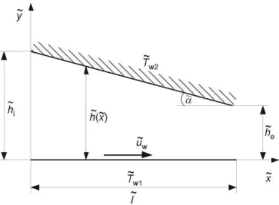
The model developed in this paper is referred to the non-isothermal microbearing gas flow with different temperatures of the walls. It is based on already verified results for an isothermal pressure-driven gas flow in a microchannel with slowly varying cross section [10] and an isothermal gas flow in a microbearing [11, 12]. The small parameter is defined as the ratio between the exit microbearing height and the microbearing length h l_e . Moreover, it is assumed that the channel cross-section varies slowly, which also implies that all physical quantities vary slowly in the flow direction. The gas flow is subsonic and the ratio between Mach and Reynolds number Ma2/Re is taken to be of the order of the small parameter. All these assumptions together with the defined relations of Reynolds, Mach, and Knudsen numbers to the small parameter e, enable a precise estimation of each term in the dimensionless governing equations, as well as in the boundary conditions. The problem is solved by the continuum governing equations (continuity, Navier-Stokes, and energy), accompanied by the Maxwell-Smoluchowski first-order velocity slip and temperature jump boundary conditions. In the solving procedure, the pressure, velocity, and temperature are expressed as the perturbation series of Knudsen number. The system of non-linear second order differential equations is obtained, and it is solved numerically. Whereas no solutions of non-isothermal gas flow in the microbearing exist in the open literature yet, the results are compared with Fukui et al. [7, 8] numerical solution of the Boltzman equation for isothermal microbearing gas flow. The obtained results appear to be in good agreement with numerical solution of the Boltzman equation for the flow conditions with no temperature differences between walls, which is a good verification of the presented solution.

Problem description

boundary condition have to be involved too. These equations are transformed into the non-dimensional form by the introduction of the following scales: the exit microbearing height h_e for crosswise co-ordinate y and microbearing height, the microbearing length l for stream-wise co-ordinate x, the wall velocity u_w for velocities, the average temperature of the lower and the upper plate

a

T for the temperature, while the pressure is scaled by the pressure at the microbearing outlet cross-section p_r and the density by

r pr

  /RT_a, where R is the gas constant. Furthermore, all non-dimensional parameters

are denoted without a bar, i. e. the pressure as p, the stream-wise velocity component as u, etc. The small parameter is defined as the ratio between the exit microbearing height and the microbearinglength:

e

h l

  (1)

The low Mach number flow conditions enable an assumption that the ratio between the square of the Mach number and the Reynolds number is of the order of the small parameter:

2 r

r

Ma Re

 _

(2)

where g = O(1),  is the ratio of specific heats, and Mar – the referent Mach number value

defined as:

w r

a

Ma

R

u

T



 (3)

and Reris the referent Reynolds number:

w e r r

a

Re R

u h p T





(4)

The dynamic viscosity



~ is assumed to be constant, i. e.



1.

The assumption of the slowly varying channel cross-section implies that the crosswise velocity component

v

~

is much smaller than the stream-wise component u, which leads to the following relation: v = eV, V = O(1).

The continuity equation, the Navier-Stokes equations for the stream-wise and crosswise directions, the energy equation, and the equation of state in the dimensionless form are:

( ) ( )

0

u V

x y





 _ _

  (5)

2

2 2

r 2

Ma u u V u p u O( )

x y x y





_    _  



 



   

  (6)

2

( )

p O

y



 

 (7)

2

2 2

r r 2

2

2 2

r

1

Ma Pr Ma Pr

( 1)Ma Pr ( )

T T p T

u V u k

x y x y

u O y

  _  _   _  _

 _{ }  _{ }

 

 

  _{ } 



 

 _ 

 

   (8)

p



T (9)

The same as the dynamic viscosity, the thermal conductivity k is treated as constant. Therefore, the Prandtl number Prc_p



/k is constant, where cp is the specific heat at

constant pressure. In accordance with the well-known Maxwell-Smoluchowski first-order slip boundary conditions, the gas velocity and the temperature at the wall in the dimensionless form are, respectively:

v

r 0

0

v 0

2 d

1 Kn , 0

d y

y

y

T u

u V

p y



 







   (10)

v

r ( )

( )

v _{( )}

2 d d ( )

Kn ,

d y h x d

y h x

y h x

T u h x

u V u

p y x













   (11)

T r

0

T 0

2 2 Kn d

1

1 Pr d

y

y

T T

T

p y





   



 



  (12)

T r

( )

T ( )

2 2 Kn d

1

1 Pr d

y h x

y h x

T T

T

p y





   



 



  (13)

where q = (Tw1 – Tw2)/2, v and T are the momentum and the thermal accommodation

coefficients, and Knr is the reference Knudsen number defined as Knrr he. Since the

molecular mean-free path is defined as   _{( R} _{T 2)}1/ 2_{/p [6], the relation between the local}

e

Kn h and the reference Knudsen number Kn_r is Kn = (T1/2/p)Knr. Furthermore, the

relation between Knr, Mar, and Rer is:

r r

r

Ma Kn

Re 2





 (14)

The presumption of an extremely subsonic flow in the slip regime enables the relation between the Mach and Knudsen numbers and the small parameter e:



Ma2_r = bem, b = O(1) and Knr = he

n

Rer = (b/g)e

m–1

, b = g2p_/2h2_{, and 2n + m = 2. The supposition of the low Mach and Knudsen}

number flow constrains m and n to the positive domain, which together with the relation 2n + + m = 2 gives that these parameters must be in the following ranges: 0 < m < 2 and 0 < n < 1. This way, two characteristic problems could be analyzed: Rer < 1, when 1< m <2 and 0 < n <

< 1/2, and Rer > 1, when 0 < m < 1 and 1/2 < n <1. In this paper, the solution for Rer > 1 is

presented. The values of the parameters m and n are chosen to enable the attendance of the inertia in the second approximation of the momentum equation, as well as the convection, dissipation and rate at which work is done in compressing the element of fluid in the second approximation of the energy equation, together with the rarefaction: m = n = 2/3. The relations for the dimensionless numbers are: Rer = (b/g)e–

1/3

, kMar 2

= be2/3, and Knr = he 2/3

. All dependant variables from eqs. (5)-(9), i. e. pressure, temperature, and velocity components, are presented in the form of perturbation series:

3 2 3 4

0 1

f  f   f O  (15)

where f0 is the solution for the flow with no-slip boundary conditions, and f1 comprises the

corrections for the slip and temperature jump on the wall. The systems of equations for two approximations, along with the corresponding boundary conditions are obtained by a substitution of the perturbation series for the pressure, velocities, and temperature in the continuity eq. (5), momentum conservation eq. (6), energy eq. (8), equation of state (9), and the boundary conditions (10)-(13). In order to capture the slip effect already in the second approximation, the power for the small parameter in the second term on the r. h. s. of eq. (15) is the same as for the Knudsen number (e2/3). As the inertia in equation (6) is of the order

2 2 3 r

Ma







, for the perturbation series in eq. (15), the inertia effect is included also in the second approximation. Also, the terms for the dissipation, convection, and rate at which work is done in compressing the elements of fluids in the energy eq. (8) are of the order

3 2 2 r

Ma





 and hence come out in the second approximation. The terms of the order O(1) and O(e2/3) are extracted, and the following sets of equations are obtained:

 for O(1)

0 0 0 0

0 0

0

p u p V

T T

x y

   

_{ } _{ }

 _  _

  (16)

2

0 0

2

d 1

d

u p

x

y



 

 (17)

2 0 2 0 T y

 

 (18)

0y ₀ 1, 0y ₀ 0

u _  V _  ₍₁₉₎

0 0 0

d ( )

0, 0

d

y h y h y h

y h

h x

u V u

x

  



   (20)

0y ₀ w1 1

0y h w2 1

T _ T  



(22)

 for O(e2/3)

0 1 0 1 0 1 0 0 1 0 1 0 1 0

2 2

0 0 0 0 0 0

0

p u p T u p u p V p T V p V

x T T T y T T T

   

 _{  }  _{  }

   

   

 _{ }  _{ } (23)

2

0 0 0 1 1

0 0 2

0

d d

p u u p u

u V

T x y x y



 _   _  





  

  (24)

2 2

0 0 0 0 1 0

0 0 0 2

0

d

1 1

Pr Pr Pr

d

p T T p T u

u V u

T x y x y y

 

   

 

  _  _  _  _    

 _{ }  _  _ 

    (25)

0

1 0 1 0

0 0

2 1

1 , 0

v y y v y u u V p y  _{ }           (26) v 0

1 1 1

v 0 0

2 1 d ( )

1 ,

d

y h y h y h

y

u h x

u V u

p y x

 _{ }             (27) 0 T 1 0

T 0 0

2 2 1

1 1 Pr y y T T p y            _

  (28)

0 T

1

T 0

2 2 1

1 1 Pr y h y h T T p y             _

  (29)

The solution procedure for each system of these equations is the same. First, the approximation of the temperature is derived from the corresponding energy equation (18) and (25) along with the temperature boundary conditions (21), (22), (28), and (29). Then, the approximation of the velocity is derived from the corresponding momentum eqs. (17) and (24) and the velocity boundary conditions (19), (20), (26), and 27). The pressure approx-imation follows from the continuity equations (16) and (23). The systems are solved successively, and the temperature, velocity and pressure analytical solutions, for the moderately high Reynolds numbers gas flow in the microbearings with different temperatures of the walls, are:

0 1 2

T a ya (30)

1 2 a h    (30a) 2 1

a  



_(30b)

2

0 1 0 2 0 3

u b T b T b (31)

2 0 2 1 1 2 4 h p b      _  _

  (31b)

2 0 3 1 1 2 4 h p b        _  _

  (31c)

3 2

0 1 0 2 0 3 0 4 0ln 0 5

V  c T c T c T c T T c (32)

2 3 3 0

1 3 0

0

1

( )

32

p h

c h p

p             (32a)

2 3 2

0 0 0

2 2 0

0 0

1

( 9)

8 2

2

h h p h p hp

c p p p      _      _  _      











(32b)





3 2 2

3

0 0 0

3 2 0 0

0 0

2 0 0 0

0

1 1 ( 1)

ln( 1) ( 1) 1 ( )

4 4 8

4

1

2

h p p h p

c hp h h p p

p p

h h p p

p p  _{ }         _{  } _{  }  _{  }  _ _  _    _  _            _{ }  _  _{ }  _{ } (32c) 3 0 0

4 2 0

0

1

4 4

h p p

c hp p       _  _      (32d) 2 2 0 5 2 1 1 4 4 h p

c  h

 

 

 _

 _  _

  (32e)

2 3 2

0 0 0

1 1

( 1) ln 2 ( ) 4 2 ( 1) ln ( ) 0

1 h p p 1 hp

           _{ }  _{ }  _{ }  _  _   _ 

    (33)

4 3 2 2

1 3 0 4 0 5 0 6 0 7 0ln 0 8 0 ln 0 9

T a T a T a T a T a T T a T T a (34)

2 2

0 1 0

3 ₃ 1 1 1 1 ₂ 1

1 1

Pr 1 Pr

( ) 4

12 12

p b p

a b a c a b

a a













        _  _

  (34a)

2

0 2 0

4 ₃ 2 1 1 2 1 2 1 ₂ 1 2

1 1

Pr 1 Pr

( ) 4

6 6

p b p

a b a b a a c a b b

a a













          _  _

  (34b)

2 2 2

0 3 0

5 3 3 1 2 2 1 3 1 4 1 2 2

1 1

Pr 3 1 Pr

2 2

2

p b p

a b a b a a c a c a b

a a













     _{ }   _    _ _  _

4 4

T 1

6 7 3

T 0

3 3 2 2

4 5 7

2 2

8

2

1 2

( 1 1 ) [(1 ) (1 ) ]

2 1 Pr

[(1 ) (1 ) ] [(1 ) (1 ) ] [1 (1 ) ln(1 )

(1 ) ln(1 )] [(1 ) ln(1 ) (1 ) ln(1 )]

a

a a a

p

a a a

a       _                               







_

_

_

_































(34d)

2 0

7 3 5 1 3 1 2 1

Pr

( )

p

a c a b a a

a 

 

  (34e)

0 8 1 Pr 2 p h a a    (34f)

4 3 2

T 1

9 3 4 5 6

T 0

2

7 8

2 2

1 (1 ) (1 ) (1 ) (1 )

1 Pr

(1 ) ln(1 ) (1 ) ln(1 )

a

a a a a a

p a a                       _{    }  

    (34g)

5 4 3 2 2 3

1 4 0 5 0 6 0 7 0 8 0 9 0ln 0 10 0 ln 0 11 0 ln 0 12

u b T b T b T b T b T b T T b T T b T T b (35)

2 0 1 1 1 1

4 ₂ 1 1 1

1 1 2

10

p b b b a

b a b c

a a





     _   _

  (35a)

2

0 1 1 2 1 2 1

5 ₂ 1 2 1 2 1 1 1 2

1 1

1

( ) 3 2 2

12

p a b b a a b

b b b a b c a b c

a a a





 _     _     _

  (35b)

2

0 1 2 1 2 1 2 1 1 3

6 ₂ 1 2 2 1 1 3 1 3 2 2 1 1 4

1 1 1

1

5

2 3 ( ) 2

3 6

p a a b b a b a b b

b a b c a b c b b b b a b c

a a a

a





  _{ }   

 _        _

  (35c)

2

0 1 2 2 1 2 1 3 1 2 3 1

7 ₂ 2 3 1 1 5 1 2 3 1 2 4 ₂

1 1 1

1 1

3

( ) 2 2

2

2 2

p a a b a a b b a b b p

b b b a b c a b c a b c

a a a

a a







 _     

 _       _

  (35d)

1

8 1 2 1 2

0

5 5 4 4 3 3

4 5 6

2 2 1 7 2 1 2 9 10 2 1

{[2 (1 ) ] 1 [2 (1 ) ] 1 }

2

[(1 ) (1 ) ] [(1 ) (1 ) ] [(1 ) (1 ) ]

[(1 ) (1 ) ]

2

[(1 ) ln(1 ) (1 ) ln(1 )] [(1 ) ln(1 ) (1

v v

a

b b b b b

p

b b b

p b a b b                              _  _                 

 

_

_

_

_





































2

3 3 1

11 ₂

1

) ln(1 )]

(1 ) ln(1 ) (1 ) ln(1 ) p

0 1 2 2 3

9 2 3 3 1 2 5

1 1

p a a b b

b b b a b c

a a   _    _   _  





(35f) 0

10 2 4

1

2

p

b b c

a

 

 (35g)

0

11 1 4

1

3

p

b b c

a

 

 (35h)





5 4 3

v 1

12 1 2 4 5 6

v 0

2 2

1

7 2 9 10

1

3 1 1 2

11 8 9 2 2

1 1

2

[2 (1 ) ] 1 (1 ) (1 ) (1 )

(1 ) (1 ) 1 ln(1 ) (1 ) ln(1 )

2

(1 ) ln(1 ) (1 ) (1 )

2

a

b b b b b b

p

p

b b b

a

p p

b b b

a a                _  _                   _   _     

 

_

_

_

_

_



























(35i)

5 5 0 4 4 0

4 1 3 5 1 4 2 3

1 1

3 3 0 11 1 8

6 1 5 2 4 3 3

1

2 2 0 1 10 1 7

7 2 1 6

1 1

(1 ) (1 ) ( ) (1 ) (1 ) ( )

5 4

(1 ) (1 )

3 3 3

(1 ) (1 )

2 2 2 2

p p

b b a b b a b a

a a

p b b a

b b a b a b a

a

p p b b a

b b a

a a           _  _      _   _   _{ }   _{ }       _    _{  }      _         _    _             





2 8

2 5 3 4

0 1

8 9 ₂ 1 9 2 6 2 7 3 5 3 8

1 1

0

9 2 7 3 8 1

2 2 0

10 1 7 2 1

2

2

(1 ) ln(1 ) (1 ) ln(1 ) ( )

(1 ) ln(1 ) (1 ) ln(1 ) (

2

b a

b a b a

p p

b b b a b a b a b a b a

a a

p

b b a b a

a

p

b b a b

a          _ _             _        _                _   _      _      _        

    ₈

3 3 0

11 1 8 1

2

0 1

12 2 2 9 3 6 3 7 2 3 9

1 1

2

1 0 1

1 3

1 1

)

(1 ) ln(1 ) (1 ) ln(1 ) ( )

3

1 2

ln (1 )

1 2 1

1

4 (1 ) ln 2 (

1 2

a

p

b b a

a

p p

b b a b a b a b a

a a

p p p

b b a a              _      _  _              _{ }       _   _{ }  _         _{ }   _                _         

 2 3

1

) ln 0

where a prime denotes d/dx, while h is the channel cross-section law defined as: h(x) = hi–

–x(hi– 1), where hi is the dimensionless parameter defined as the ratio of the inlet and outlet

microbearing heights hi = h hi/ .e Based on the coefficient g that is defined from eqs. (1)-(4) as g =



_wl p h/ _{e e}2and the bearing number L = 6



u l p h_{w e e}2, is evident the relation g = L/6.

The system of the two second order differential eqs. (33) and (36) that enables the prediction of the pressure along the microbearing, demands four boundary conditions at the channel inlet – p0, p1,

p

0



, and

p

1



. However, the first derivate of the pressure is unknown.

This problem is overcome by using the known pressure at the channel outlet instead of the first pressure derivate at the inlet, which imposes the application of the shooting method for the solving of the system of equations. The boundary conditions for the pressure, prescribed at the inlet and outlet are: x = 0, p = p0 = 1, p1 = 0, and x = 1, p = p0 = 1, p1 = 0.

Results and discussion

The results for the pressure, velocity, and temperature field for different temperature walls microbearing gas flows are presented in this section. The problem is defined by five dimensionless parameters. Here, the following five have been selected: the reference Knudsen and Mach number, half of the dimensionless temperature difference between the lower and upper wall θ, the bearing number L, and the ratio between the inlet and exit microbearing heights h1. All results are obtained for v= 1, T = 1, and for a monoatomic gas, thus = 5/3

and Pr = 2/3.

In fig. 2, the pressure distribution for a microbearing with constant and equal temperatures of the walls (q = 0) with and without the second order effects (inertia, convection, dissipation, and rate at which work is done in compressing the element of fluid) are presented. Those are compared with a numerical solution of the Boltzmann equation (Fukui et al. [7, 8]) and an analytical solution with two approximations (Stevanovic [11]) which are obtained for an isothermal microbearing gas flow without inertia effects. Excellent agreement is achieved. For Kn = 0.1, a deviation from the numerical solution exists, which is a consequence of only two approximations in the presented model, while good agreement is attained for lower Knudsen numbers.

The walls’ temperature influence on the pressure distribution along the microbearing is presented in fig. 3. The temperature difference between the walls for two analyzed regimes is the same, but the position of the warmer wall is different. The upper location of the warmer wall (q = –0.5) leads to a higher pressure i. e. a higher microbearing load carrying capacity than for the lower location of the warmer wall (q = 0.5)

Figure 2. Comparison of the presented results for the pressure distribution in microbearing with equal temperatures of the walls with those of Fukui et al. _{[7, 8] and of Stevanovi}ć _{[11] for} the flow condition h_{i = 2,} L _{= 1, Mar = 0.3, and}

case. Also, the influence of the second order effects that come out from the momentum and energy equations on the pressure distribution along the microbearing are presented in fig. 3. These effects (inertia, convection, dissipation, and rate at which work is done in compressing the element of fluid), without the second order effects that come out from the boundary conditions (slip and temperature jump), would be marked in all figures in this paper as “the second order effects.” It is evident that “the second order effects” lead to pressure increase in the microbearing, as well as to a higher load carrying capacity.

In order to analyze the influence of the slip and temperature jump at the wall on pressure distribution in microbearing, beside the results for Kn = 0.1, the results obtained for the continuum flow condition (Kn = 0) are presented in fig. 3 as well. It is obvious that these second order effects that appear in the boundary conditions at the wall lead to a lower pressure in the microbearing. The influence of the warmer wall position on the pressure distribution is the same for the continuum as for the slip flow conditions. When the wormer wall is above, the pressure is higher than when the wormer wall position is underneath.

Figure 3. The walls’ temperatures influence on

the pressure distribution along the microbearing for: h_i = 2, L = 1, Mar = 0.3, Knr = 0.1 and three temperature boundary conditions: q = 0.5, q = 0, and q = –0.5

Figure 4. The walls’ temperature influence on the

velocity field in the microbearing for h_i = 2, L _{= 1,}

Mar = 0.3, Knr = 0.1 and three temperature boundary conditions: q _{= 0.5,} q _{= 0, and} q ₌ –_0.5

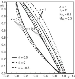
In fig. 4, the influence of the temperature boundary conditions on the velocity profiles for the flow condition defined with Knr = 0.1, hi = 2, L = 1, Mar = 0.3 are presented.

The full lines refer to the upper location of the warmer wall (q = –0.5), the dash-dotted lines to the equal wall temperature (q = 0), while the dashed lines refer to the lower position of the warmer wall (q = 0.5). In any case, the slip at the lower wall decreases from the inlet to the exit, while at the upper wall the slip is increasing. For both presented temperature boundary conditions, the velocity becomes higher from the microbearing inlet to its exit.

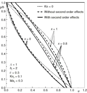
The influence of the second order effects, as well as the rarefaction effect on the velocity in the microbearing is presented in fig. 5. The inertia, convection, dissipation, and rate at which work is done in compressing the element of fluid lead to lower velocity values for the flow conditions defined with Knr = 0.1, hi = 2, L = 1, Mar = 0.3, and q = 0.5, but have

conditions (26) and (27), and the solution for u0 (31) that does not depend on the

second order effects. The results for Kn = = 0 are also presented in fig. 5 with dotted lines. These results are the first order solution u0 (31) which excludes the

rarefaction as well as the second order effects from the momentum and energy equations. The difference between the velocity profiles obtained by omitting all second order effects (u0), obtained by

excluding only the second order effects from the momentum and energy equa-tions –b = 0 in eqs. (24) and (25), i. e. in solutions (34) and (35) – and obtained with the rarefaction as well as the second order effects from the momentum and energy equations –b¹ _{0 in eqs. (24) and}

(25), i. e. in solutions (34) and (35) – is evident.

The temperature profiles for the microbearing gas flow between the walls at different temperatures are depicted in fig. 6. The results are given for the Knudsen number Knr = 0.1, Mach number Mar = 0.3, bearing number L = 1, the ratio of the inlet and outlet

microbearing heights hi = 2, and for twodifferent temperature boundary conditions. For both

presented cases, the temperature difference is the same, but in fig. 6(a) the lower wall is warmer (q = 0.5), while in fig. 6(b) it is colder (q = –0.5). The complete temperature solution

Figure 5. The rarefaction influence and the second order effects influence on the velocity field in the microbearing for h_i = 2, L _{= 1, Mar = 0.3, Knr = 0.1,}

and q _{= 0.5}

Figure 6. The temperature profiles for the microbearing gas flow for h_i = 2, L _{= 1, Mar = 0.3,}

obtained by eq. (35) is illustrated as well as the solution without the second order momentum and energy effects – obtained by putting b = 0 in eq. (35) – and the deviation between them is negligible. The temperature jump is the same for both solutions and it is larger at the warmer wall than at the colder in one cross-section. It always increases from the inlet to the exit. The gas temperature always decreases from the wormer towards the colder plate and is different from the linear temperature distribution. Also, the first approximation, i. e. the solution for the continuum, eq. (30), which excludes any second order effect, are presented in fig. 6. In that case, the temperature profile is the same in any cross-section. The rarefaction influence on the temperature profile decreases the temperature differences in the microbearing cross-section.

Conclusions

The presented perturbation method enables obtaining a non-isothermal analytical solution for a microbearing gas flow, which had not been presented in literature before. The pressure, velocity, and temperature fields for the moderately high Reynolds number flow conditions and different walls temperatures have been analyzed. The small parameter has been defined by eq. (1) and Mach, Knudsen, and Reynolds numbers have been expressed with it. Furthermore, the exact relation between these numbers has been used for a precise estimation of the contribution of each term in the momentum and energy equations, as well as in the boundary conditions. The pressure, velocity, and temperature have been described with perturbation series. The first approximation corresponds to the continuum flow conditions, while the second approximation represents the contribution of the rarefaction effect. In addition, for the moderately high Reynolds numbers, from the second approximation the inertia, convection, dissipation, and rate at which work is done in compressing the element of fluid have been included.

The rarefaction influence, as well as the influence of the second order effects from the momentum and energy equations on the pressure, velocity, and temperature fields has been analysed. The rarefaction causes a lower pressure in the microbearing, while the second order effects from the momentum and energy equations increase the pressure in the microbearing. The temperatures of the walls also influence the pressure. For the same temperature difference between the walls but the opposite positions of the warmer wall, the pressure is higher when the warmer wall is above.

The rarefaction has influence also on the velocity and temperature fields. The velocity slip and the temperature jump are always present in the solution. For the solution with two approximations, they are equal, regardless of whether the second order effects are incorporated or not. However, the second order effects have influence on the velocity and temperature profiles.

The first approximation is the solution for the continuum flow conditions without the second order effects. It is applicable for a non-isothermal gas flow in classic bearings with different temperature of the walls. In that case, the temperature profile does not change along the bearing, while the velocity does.

References

[1] Gad-El-Hak, M., The MEMS Handbook, CRC Press, Boca Raton, Fla., USA, 2002

[2] Burgdorfer, A., The Influence of the Molecular Mean Free Path on the Performance of Hydrodynamic Gas Lubricated Bearing, J. Basic Eng., 81 (1959), 1, pp. 94-100

[3] Mitsuya, Y., Modified Reynolds Equation for Ultra-Thin Film Gas Lubrication Using 1.5-Order Slip-Flow Model and Considering Surface Accommodation Coefficient, ASME J. Tribology, 115 (1993), 2, pp. 289-294

[4] Hsia, Y., Domoto, G., An Experimental Investigation of Molecular Rarefaction Effects in Gas-Lubricated Bearings at Ultra Low Clearances, J. Lubr. Technol, 105 (1983), 1, pp. 120-130

[5] Sun,Y. H., Chan, W. K., Liu, N. Y., A Slip Model for Gas Lubrication Based on an Effective Viscosity Concept, J. Eng Tribol, 217 (2003), 3, pp. 187-195

[6] Bahukudumbi, P., Beskok, A., A Phenomenological Lubrication Model for the Entire Knudsen Regime,

J. Micromech and Microeng, 13 (2003), 6, pp. 873-884

[7] Fukui, S., Kaneko, R., Analysis of Ultra-Thin Gas Film Lubrication Based on Linearized Boltzmann Equation: First Report-Derivation of a Generalized Lubrication Equation Including Thermal Creep Flow, J. Tribol, 110 (1988), 2, pp. 253-262

[8] Fukui, S., Kaneko, R. V., A Database for Interpolation of Poiseuille Flow Rates for High Knudsen Number Lubrication Problems, J. Tribol, 112 (1990), 1, pp. 78-83

[9] Liu, N., Ng, E. Y. K., The Posture Effects of a Slider Air Bearing on its Performance with a Direct Simulation Monte Carlo Method, J. Micromech. Microeng, 11 (2001), 5, pp. 463-473

[10] Stevanovic, N., A New Analytical Solution of Microchannel Gas Flow, J. Micromech. Microeng, 17

(2007), 8, pp. 1695-1702

[11] Stevanovic, N., Analytical Solution of Gas Lubricated Slider Microbearing, Microfluid, Nanofluid, 7

(2009), 1, pp. 97-105

[12] Stevanovic, N., Milicev, S., A Constant Wall Temperature Microbearing Gas Flow, FME Transactions, 38 (2010), 2, pp. 65-71