Lat. Am. j. solids struct. vol.11 número8

Abstract

In this work it is presented a coupling between the Boundary Ele‐ ment Method BEM and the Finite Element Method FEM for two‐ dimensional elastostatic analysis of frame‐solid interaction. The BEM is used to model the matrix while the reinforcement is modeled by the FEM. Regarding the coupling formulation a third degree polyno‐ mial is adopted to describe the displacement and rotations of the reinforcement, while a linear polynomial is used to describe the contact force among the domain matrix and the reinforcement. Perfect bounding contact forces are improved by means of redun‐ dant equations and Least squares method. Slip‐bounding with two and three paths written as function of relative displacement are used to calculate the transmitted contact forces. Examples are used to demonstrate that the proposed slip‐bounding procedure regularizes the contact force behavior.

Keywords

Boundary Element Method, Finite Element Method, BEM/FEM cou‐ pling, adherence models.

Sliding frame‐solid interaction using BEM/FEM coupling

INTRODUCTION

The combination of the finite element method FEM and boundary element method BEM to solve structural analysis is attractive because it allows for an optimal exploitation of the respective advantage of the methods Zienkiewicz et al., . The main strength of the BEM for boundary‐value problems governed by linear, homogenous, and elliptic differential equations with constant coefficients is the reduction of the dimensionality of the problem by one unit for linear constitutive relations Brebbia, ; Brebbia, . Particularly, BEM is useful to model special situations such as very large or un‐ bounded domains, geometrical singularities e. g. cracks or to obtain very accurate results in regions of complicated shape Aliabadi, ; Bonnet, ; Frangi et al., . Thus, coupling the BEM and the FEM allows exploiting their complementary advantages. By the other hand, the FEM is appropriate to solve a lot of problems, including e. g. those with heterogeneous or non‐linear constitutive properties, or finite deformations.

The idea of combining these two methods goes back to Zienkiewicz et al. . One branch of BEM/FEM coupling is the iterative coupling in which the individual sub‐domains are treated inde‐ pendently by either method. The procedure starts with an initial guess of the interface unknowns that will be improved by solving each sub‐domain and returned to interface. This procedure repeats until an error tolerance is achieved. Although this iterative coupling is very attractive to software design, its convergence commonly depends on relaxation parameters which are rather empirical Estorff and Hagen, . For this reason, a direct coupling approach is adopted in this work.

Standard BEM formulations to deal with solids stiffened by bars or fibers are derived by combining the BEM and FEM algebraic equations. The domain continuum or matrix is analyzed by BEM, while

Fabio Carlos da Rocha a

Wilson Sergio Venturini b

Humberto Breves Coda c

a,b,c_{University of São Paulo, School of}

Engineering of São Carlos, Department of Structural Engineering, Av. Trabalhador SãoCarlense, , ‐ São Carlos‐ SP, Brazil;

a_{Federal University of Sergipe, Depart‐}

ment of Civil Engineering, Av. Marechal Rondon, s/n, ‐ São Cristovão‐ SE, Brazil;

Latin American Journal of Solids and Structures ‐ finite elements are used to represent inclusions bars for instance . The coupling is always done by enforcing displacement compatibility and traction equilibrium at interface nodes. Practical applications for non‐slipping or slipping coupling using BEM/FEM coupling are presented, for instance, in Beer and Watson , Coda and Venturini , Coda , Leite et al. , Botta and Venturini

, , Leonel , Rocha .

As contribution, the present work is able to capture bending effects in the analysis of frame‐solid interaction, which includes bending stiffness in reinforcements immersed in D continuum. For this purpose, in this study it is adopted a Rissner‐Mindlin type frame finite element with third order of ap‐ proximation for both displacement and rotations resulting in four nodes and degrees of freedom. However, the contact force is modeled by linear approximation resulting in only independent values which leads to a not square force matrix. These approximations displacements and tractions were used because it is the lowest order that satisfies the differential equation governing the problem. In this approach, the boundary element force lines are build in a compatible way, that is there are source points generating a third order approximation for displacements, but the contact force approximation is linear, also resulting in a not square force matrix.

The least Squares technique is used to eliminate the dependent equations due to the above men‐ tioned difference in approximation order for displacement and tractions. Moreover some authors, Botta and Venturini , and Leonel , claim that this procedure reduces contact force oscilla‐ tions.

This paper is organized as follows. It is presented in section the FEM formulation to model the frame structure, which is shown the kinematics adopted. In section is shown the BEM formulation adapted to domain modeling. In section it is presented the proposed coupling formulation between BEM and FEM considering both perfect bonding and debonding cases. This section is divided in subsec‐ tion . in which there are presented the basic equations to perfect bonding and an example to verify this formulation. In sub‐section . it is presented the coupling formulation considering the slip be‐ tween reinforcement and domain. Debonding models, basic equations and the non‐linear formulation to solve slipping are presented in sub‐sections . . , . . and . . , respectively. The sub‐section . presents two examples. The first simulates a pullout test and the second solve a soil‐structure interac‐ tion case. Finally, in section the final remarks and conclusions are given.

THE FRAME ELMENT MODELING – FEM FORMULATION

As mentioned before, the FEM is used to model frame elements and structures. Here, elements which have three degrees of freedom per node and cubic approximation for displacement and rotation are employed. This way, the elements have four nodes and these nodes present two translations verti‐ cal and horizontal and one rotation. Moreover, the distributed applied forces will follow linear approx‐ imation.

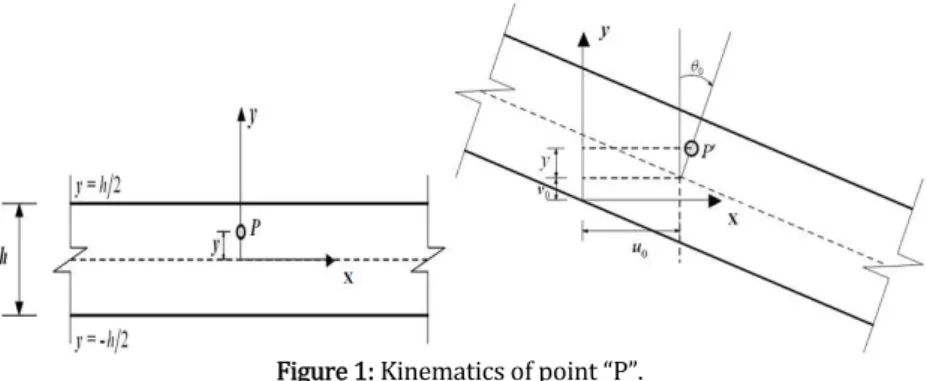
. Kinematics

For any point on the structure, the horizontal and vertical components of displacements are given by, respectively:

(

)

( )

( )

( )

( )

= +

=

0 0

0 ,

, ,

p p

U x y U x x y

V x y V x

q

where

x

and

y

are the reference system in the center of the layer, as shown in figure and

U

p and p

Latin American Journal of Solids and Structures ‐

Figure : Kinematics of point P .

From equation , one can apply the differential operator to obtain the linear strain components:

( )

( )

( )

( )

( )

( )

(

)

( )

( )

( )

( )

¶ ¶ ¶ = = + ¶ ¶ ¶ ¶ = = ¶

æ¶ ¶ ö_÷ æ ¶ ö_÷

ç _÷ ç _÷

ç ç

= _ç + _÷÷= _ç + _÷

÷÷

ç ¶ ¶ ÷ çè ¶ ø

è ø 0 0 0 0 , , , , 0 , , 1 1 , . 2 2 p x p y p p xy

U x y U x x

x y y

x x x

V x y x y

y

U x y V x y V x

x y x

y x x

q e

e

e q

Applying the constitutive law for the isotropic materials, the stress components at the point p are obtained:

( )

( )

( )

( )

(

)

(

)

(

)

(

)

( )

( )

æ¶ ¶ ö_÷

ç _÷

ç

= = _ç + _÷÷÷

ç ¶ ¶

è ø

= =

æ _¶ ö_÷

ç _÷

ç

= = _ç + _÷

÷÷ ç ¶ è ø 0 0 0 0 , ,

, , 0

, , ,

2

x x

y y

xy xy

U x x

x y E x y E y

x x

x y E x y

V x G

x y G x y x

x

q

s e

s e

t e q

where E and G are the longitudinal and shear elastic moduli, respectively.

To write the equilibrium equation it is used the Principle of Minimum Total Potential Energy. Using equations and one writes the Total Potential Energy equation as,

( )

( )

( )

( )

(

)

- =

-æ é _{æ ö æ ö} ù ö_÷

ç _{ê ç} ¶ _{÷ ç}¶ ¶ _{÷ ú ÷}

ç _{ç ÷ ç ÷ ÷}

= ç_çç ê_{ê çç} + _{¶ ÷÷}÷ + _{çç ¶} + _¶ ÷_{÷÷ ú}ú _÷÷ ÷

è ø è ø ÷

çè êë úû ø

= +

ò ò

ò

2 2

1 _{0 0 0}

0 ₂ 1 1 0 0 1 2 4 , e p e _A

p x y

U U

V _E U

U G y dA d

L L

U t U t V dA

x x q x

q x x

x x x

where Ue and Up are the internal and potential energy of external forces, tx and ty are the compo‐ nents of the distributed loading contact tractions applied to the structure, L and A are the length and cross sectional area of the frame element, respectively. For approximate unknowns U0, V0 e q0

Latin American Journal of Solids and Structures ‐

( )

( )

( )

( )

( )

= = =

= =

= = =

= =

å

å

å

å

å

4 4 4

0 0 0 0 0 0

1 1 1

2 2

1 1

, ,

,

i i i

i i i

i i i

j j

x j x y j y

i i

U u V v

t t t t

j x j x q j x q

y x y x

with 0 i

u , v₀i e q₀i being the nodal values unknown . Since j x_i

( )

and y x_j

( )

are shape functions:

( )

_{= -} æç_{ç + ÷}öæ÷_÷çç _{- ÷}÷ö_÷

(

_-

)

( )

_{= +}

(

₊

)

_ççæ _{- ÷}÷ö_÷

(

_-

)

ç ÷ç ÷ ç ÷

è øè ø è ø

1 2

9 1 1 27 1

1 , 1 1

16 3 3 16 3

j x x x x j x x x x

( )

_{= -}

(

₊

)

_çæç _{+ ÷}÷ö_÷

(

_-

)

( )

_{= +} æ_çç ₊ öæ÷_÷÷çç _{- ÷}÷ö_÷

(

₊

)

ç ÷ ç ÷ç ÷

è ø è øè ø

3 4

27 1 9 1 1

1 1 , 1

16 3 16 3 3

j x x x x j x x x x

( )

= -

( )

= + - £ £

1 2

1 1

, 1 1

2 2 and

x x

y x y x x

Minimizing the energy functional, equation , one finds the algebraic equilibrium system given by:

  =   + 

3 ,3 3 ,1 3 ,2 extr_{2 extr,1} 3 ,1

E E E E

NF NF NF NF NF NF NF

K U G f F

where: _KE _{is stiffness matrix, G}E _{is equivalence forcematrix, U}E _{unknown vector with displace‐} ments and rotations, _fE _{is the vector containing the nodal values of the distributed load, F is the} concentrated force. Labels NF and NF_extr are node numbers for the displacements and rotations , four per element, and node numbers for forces two per element , respectively

THE DOMAIN MODELING – BEM FORMULATION

Let us consider the domain

W

and its boundary

G

. For an elastic body defined by the domain

W

, the equilibrium equation, written in terms of displacements, is given by:

(

)

 +  ⋅  + =

-2 1 ₀

1 2n G

b

u u

where

u

represents the displacement vector,

G

_{is the shear modulus and} n is the Poisson’s ratio. For a domain

W

with boundary

G

, the integral representation of displacements is derived by ap‐ plying reciprocity theorem or Green’s second identity .

G G

⋅ = -

_ò

* ⋅ _dG +

_ò

* ⋅ _dG

c u P u U p

Where the symbols * is used to indicate fundamental solution equation and

p

represent bound‐

Latin American Journal of Solids and Structures ‐

(

)

(

)

(

)

(

)

{

(

) (

)

(

)(

)

}

ì - ü

ï ï

ï_{é ù} ï

= - _- í_ïë - _û - Ä + ý_ï

ï ï

î þ

é ù

= - ⋅ _ë - + Ä _û+ - Ä - Ä

-*

*

7 8 1

ˆ ˆ 3 4 ln

8 1 2

1

ˆ ˆ 1 2 2ˆ ˆ 1 2 ˆ ˆ ˆ ˆ

4 1

r G

r

n n

p n

n n

p n

U I r r I

P n r I r r n r r n

where

r

ˆ

=

r r

i

=

r

,i with r being the distance between the source and field points,

( )

1 2

i i

r

=

r r

, r_i are

components of the vector r,

n

ˆ

is the boundary normal unit vector and

I

is the second order identity

tensor or Kronecker delta .

For numerical solution,

u

and

p

are approximate by polynomial functions over boundary ele‐

ments, in this work linear polynomials are used for boundary elements internal force lines are further discussed , and the integral equation is converted into an equivalent algebraic system as follows:

=

U P

H G

where matrix

H

is obtained from the left terms in equation and matrix

G

_{from the terms on the}

right side.

U

_{is a vector which contains the nodal values of displacements for all boundary nodes and}

P

is the nodal traction vector.

After substitution of the prescribed boundary conditions, the algebraic equations may be written as

= =

X Y

A B F

The vector

X

contains all the unknown boundary displacements and tractions,

A

is a coefficient ma‐

trix which is usually non‐symmetric and densely populated, and

B

is a matrix which contains the coef‐

ficients corresponding to the prescribed boundary conditions

Y

.

One can differentiate equation to derive the integral representation of strains and then apply the Hooke’s law to obtain the stress integral equation, written for internal points, as follows,

G G

= -

_ò

_S* ⋅_udG +

_ò

_D*⋅_pdG

s

Where _S* _{and D}* _{are well known third‐order tensor for the stress equation obtained by applying the} Hooke’s law on the fundamental solution at the source point Brebbia and Domingues, .

BEM/FEM COUPLING FORMULATION

In this section, additional terms inserted in the classical formulations of BEM and FEM as well as the coupling between BEM and FEM are shown.

. Basic equations – perfect bonding

In this subsection the perfect bounding situation is described. It implies a direct compatibility be‐ tween displacements and contact force equilibrium or continuity . Thus:

= -R D

f f

=

D R

U QU

Where R

U

and

U

D are vectors containing nodal displacements for frame element and domain, re‐ spectively; R

f

and

f

D are nodal distributed force vector applied on the frame finite elements and on the force line boundary element in the D domain , respectively. Once vector R

Latin American Journal of Solids and Structures ‐ ponents two translations and one rotation and vector D

U

contains two components two transla‐ tions , the correlation between these two vectors is done by

Q

matrix.

The components of the vectors

U U

R

,

D

,

f

R and

f

Dare shown in figure .

Figure : Force and displacement approximation at frame interface. For D solids the unknown forces, D

f

, would be distributed over internal surfaces. For D solids this forces appears distributed along internal lines, which, roughly, work as internal boundaries dedi‐ cated only for tractions. Thus, the integral equation is modified to include the additional term:

G G G

⋅ = -

_ò

*⋅ G +

_ò

*⋅ G +

_ò

*⋅ G

R

D R

d d d

c u P u U p U f

where _fD_{is the internal force acting along the interface, G}

R, between the two materials and repre‐

sents the fiber effect applied in the domain. Similarly, the integral equation including this addi‐ tional effect is written as:

G G G

= -

ò

*⋅ G +

ò

*⋅ G +

ò

*⋅ G

R

D R

d d d

s S u D p D f

Latin American Journal of Solids and Structures ‐

= + D

bbUb bb bP brf

H G G

= - + +

D D

rb b rb b rr

U H U G P G f

where index b denotes boundary and index r denotes frame, respectively. Additionally, the first index

denotes source points and the second index denotes field points, which, are on boundary or load line. The superimposed frame element reinforcement and load line representations can be seen in figure in which

n

elements finite and line are employed. The displacement nodes for each finite element are represented by squares and crosses represent the collocation points of equation where displacements are calculated. It is observed that for fiber ends BEM equations are not written in the same position of the finite element nodes to avoid singularities; however displacements are extrap‐ olated to the nodal positions in order to make them compatible. Moreover, this modeling allows the reinforcement frame ends to reach the body boundary without interfering in basic BEM equations.

Figure : Compatibility between BEM and FEM nodes. Therefore, the displacement compatibility is rewritten as:

= =

 D R

U TU

T TQ

Where _Tˆ _{is the matrix that relates the nodal positions and direction of the U}D _{vector with the U}R vector. Furthermore, the T matrix has dimension 3NF columns by 2N_int rows, for which N_int is the

amount of BEM interface points.

According to figure , the amount of finite element nodes is equal to the amount of boundary inter‐ face nodes, i. e. NF =Nint, therefore the determination of the coupling parameters and the boundary values can be summarized by the following system of equations:

     

      

    

ìïï

ï _{= +}

ïï ïï

ïïï _{+ = +}

íï ïï ï

= +

î

int

int

int int

int int int int int 2 ,1 2 ,2 2 ,1 2 ,2 2 ,1 2 ,2

2 ,1 _{2 ,2 2 ,1}

2 ,2 2 ,1 2 ,2 2 ,1

3 ,3 3 ,1 3 ,3 3 ,1 3 ,1

extr extr

extr extr

extr extr

D bb b bb b br

N N N N N N N N N

D D

rb b rb b rr

N _{N NF NF}

N N N N N N

R R R R

N N N N NF _NF N

U P f

U U P f

K U G f F

H G G

H G G

Latin American Journal of Solids and Structures ‐ The N1 values of Ub and N2 values of Pb are known on G1 and G2

(

G = G +G

1 2

)

respectively, hence there are only 2 N unknowns in the system of equations . As usual, to introduce these boundary conditions into one has to rearrange the system by moving columns of Hbb, Hrb with

bb

G , G_rb from one side to the other, respectively. Once all unknowns are passed to the left‐hand side and applying conditions of equations and one can write the new system of equations as:

     

       

   _ 

ìïï

ï _{= +}

+ = +

í

= - +



int int int

int int int

int int int int int

2 ,1 _{2 ,1}

2 ,2 2 ,2 2 ,1 2 ,2

2 ,3 3 ,1

2 ,1 _{2 ,2 2 ,2 2 ,1}

2 ,2 2 ,1

3 ,3 3 ,1 3 ,2 _{2 ,1} 3 ,1

extr extr extr extr extr _extr D bb bb b br

N _N

N N N N N N N

R D

rb rb b rr

N N N

N _{N N N NF NF}

N N N

R R R D

N N N N NF _NF N

X F f

X T U F f

K U G f F

A B G

A B G

ïï ïï ïïï ïï ïï ïï ïï ïïî Or in matrix form,

 

{ }

_

{ }

+ +

+ + + + +

ì ü

é - ù ï_ï ï_ï é ù ìï_ï üï_ï

ê ú _{ïï ïï} ê ú _{ï ï}

ê ú ï_í ï_{ý =} ê ú ₊ ï_í ï_ý

ê ú _{ï ï} ê ú _{ï ï}

ê _- ú ï_ï ï_ï ê ú ï_ï ï_ï

ê ú _{ï ï} ê_ë ú_{û ïî ïþ}

ë û ïî ïþ





int i

int int int

2 ,1

2 5 ,2 2 5

2 5 ,2 3 2 2 3 2 ,1

0 0

0 0

0

extr extr

bb br bb

R R R

b

D _N

rb rb rr

N N N N N N N N N NF N N NF

X

K G U F F

T f

A G B

B

A G

 nt,1

As described above, at the fiber element level, the number of displacement values is larger than the number of bonding or contact force nodal values. This occurs because in equation the number of algebraic relations is much larger than the number of force values in D

f . To reduce the number of

equations to the same as the number of unknowns one can apply the Least Square Method LSM . In this work the LSM is applied over equation or , as follows:

   +   =    +    int

int int int int int int int

2 ,1 _{2 ,1}

2 extr,2 2 ,2 2 ,1 2 extr,2 2 extr,2 2 ,2 2 ,1 2 extr,2 2 ,2 extr extr

D D

rr rb b rr rr rb b rr rr

N _NF

NF N N N N NF N NF N N N N NF N N NF

U U P f

G H G G G G G

Or,

   +    =    +    int int int

int int 2 ,1 int2 ,3 3 ,1 int int int int 2 ,1

2 extr,2 2 ,2 2 extr,2 2 extr,2 2 ,2 2 ,1 2 extr,2 2 ,2 extr extr

R D

rr rb rr rr rb b rr rr

N N N

N _NF

NF N N N NF N NF N N N N NF N N NF

X T U F f

G A G G B G G

Where the matrix Grr defined for each fiber and



rr

G is the transpose matrix ofG_rr, i.e. G_rr =G_rrT.

Therefore, the system of equations turns into a square system as:



+ +

+ + + + + +

ì ü

é - ù ï_ï ï_ï é ù

ê ú _{ï ï} ê ú

ï ï

ê ú ï_í ï_{ý =} ê ú

ê ú _{ï ï} ê ú

ê _- ú ï_ï ï_ï ê ú

ê ú _{ï ï} ê_ë ú_û

ë û ïî ïþ

    



int

int int int 2 3 2 ,

2 3 2 ,2 3 2 2 3 2 ,1

0

0 0

extr extr extr extr

bb br bb

R R R

D

rr rb rr rr rr rr rb N N NF N N NF N N NF N N NF

X

K G U

T f

A G B

G A G G G G B

{ }

_

{ }

+ + ì ü ï ï ï ï ï ï ï ï

+ í_ï ý_ï

ï ï

ï ï

ï ï

î_{}þ 

int 2 ,1

2 3 2 ,1

2 0 0 extr b N

N N NF N

Latin American Journal of Solids and Structures ‐ . Numerical example – perfect bonding

In this section, one numerical example is analyzed to check the performance and accuracy of the proposed BEM/FEM coupling for two‐dimensional reinforced solids.

The reinforced simple supported beam subjected to homogeneous transversal surface load 7

10

q= - N , shown in figure , is analyzed. This plane structure is five meter length

( )

L

, one meter

height

(

H

)

and the position of the reinforcement is centimeter(h0) from the lower part of the ma‐ trix and is four meters long L0 . The following properties for domain

( )

D

and reinforcement

( )

R

are considered: Elasticity modulus ED =2.8

10 2

10 N m and ER=2.8

11 2

10 N m , Poisson’s ration

0.2 D

n = and n =0.0, inertia moment IR=1.78891

7 4

10 m

- and cross‐sectional area SR =1.29

2 2

10 m

- .

Figure : Geometry of the structure under analysis.

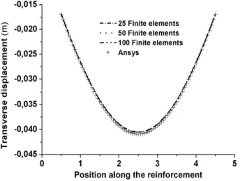
The beam is discretized by linear boundary elements with the same length. Three discretiza‐ tions are employed to model the reinforcement, with , and finite elements. The same number of force line BEM elements is employed to model the interface. The results are compared with the commercial software ANSYS employing BEAM elements to model the reinforcement and PLANE D solid elements to model the domain. Figures , and compare results axial, transverse displacements and rotations achieved using the BEM/FEM coupling discretizations and ANSYS.

Latin American Journal of Solids and Structures ‐ Figure : Transverse displacement graphics on interface, BEM/FEM.

Figure : Graphic shows the rotation on interface, BEM/FEM.

The above results make evident that even the poorest BEM/FEM coupling discretization has good accuracy when compared with the reference result.

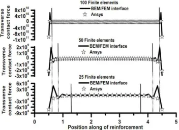
Regarding tractions at the interface, the BEM/FEM results can be seen in Figures and .

Latin American Journal of Solids and Structures ‐

Figure : Transverse contact force graphics on interface, BEM/FEM.

According to Figures and , for perfect bonded elastic reinforcement, it’s observed that for the three BEM/FEM discretizations there is a perturbation in the traction values at the ends of the fiber. The behavior of axial forces, as shown in Figure , had been observed by Botta and Venturini , however, the behavior shown in Figure has not been reported before. Moreover, the use of LSM par‐ tially smoothes the behavior of contact force when compared with results that do not apply this strate‐ gy for the coupling, Leite et al. . At this point an important result of this study should be ad‐ vanced; when debondig is allowed always occurs in a small vicinity of infinity contact stress the above perturbation disappears.

When using nonlinear constitutive relations for matrix, there are evidences of smooth solutions for this kind of problems which were reported by Coda . Moreover, one may note, in Figure , that the extension of the contact force perturbation reduces as discretization increases.

. Coupling formulation – debonding

In this section, the previous coupling is extended to accomplish debonding. The adopted models to represent debonding as well as the nonlinear formulation to simulate the slip between domain and frame elements are presented. The feasibility of this formulation is shown through numerical examples.

. . Debonding models

Fibers embedded in the domain play an important role to improve solid stiffness and loading capaci‐ ty if enough internal forces along the interface can be sustained. Sliding along the interface may be al‐ lowed when a certain amount of strength is preserved. The ideal situation for which perfect bonding is assumed, as shown in previous section, is impossible in practice; at least in the vicinity of fiber ends, as the interface forces approach the infinity Radtke et al, . Therefore, a certain amount of sliding occurs according to the bonding carrying capacity.

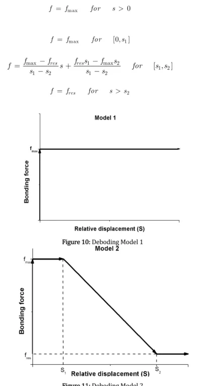
Latin American Journal of Solids and Structures ‐ From the Figure and , the following relationships are written for the adopted models, respec‐ tively:

Model

max 0

f = f for s >

Model

max [0, 1]

f = f for s

max 1 max 2

1 2

1 2 1 2

[ , ] res res

f f f s f s

f s for s s

s s s s

-

-= +

-

-2 res

f = f for s >s

Figure : Deboding Model

Latin American Journal of Solids and Structures ‐ . . Basic equations

The slip consideration introduces a new variable in equations . This new variable represents the relative displacement,

s

, between the domain and frame elements. The compatibility equations are now expressed by:

( )

= -D R

f f s

=  +

D R

U TU TS

Where vector S contains the nodal relative displacement values, T relates the nodal positions UD with S . Furthermore, T matrix has dimension 2NF_extr columns by 2N_int rows. The other terms in equations and have already been explained, but now tractions on interface depend on rela‐ tive displacements

s

. In this work, D

U

and

U

R have been approximated by cubic polynomial and S

by linear polynomial.

From the introduction of relative displacements, the equilibrium equation of the boundary element method may be rewritten as:

+ = - + +

 _{R D}

rb b rb b rr

TU TS H U G P G f

Therefore, the BEM coupling equation can be rewritten as,:

    

( )

        

( )

 = + + + = +    int int int int

int

int int

int int in

2 ,2 2 ,1 2 ,2 2 ,1 2 ,2 2 ,1

2 ,3 3 ,1 2 ,2 2 ,1 _{2 ,2}

2 ,2 2 ,1 2 ,2 2 ,1 2 ,1

3 ,3 3

extr extr

extr extr

extr extr

R bb b bb b br N N N N N N N NF NF

R R

rb b rb b rr

N N N N NF NF _{N NF}

N N N N N N NF

R R N N N

U P f s

U T U T S P f s

K U

H G G

H G G

 

( )

 ìïï ïï ïï ïï ïï íï ïï ïï

ï = +

ïï

ïïî t,1 3 int,2 extr₂_,1 3 int,1

extr

R R

N NF N

NF

G f s F

Applying boundary conditions, the equation results:

    

( )

        

( )

 = + + + = +    int int int int

int int int

int int int 2 ,1

2 ,2 2 ,2 2 ,1 2 ,2 2 ,1

2 ,3 3 ,1 2 ,2 2 ,1

2 ,1 _{2 ,2 2 ,2}

2 ,2 2 ,1 2 ,1

3 ,3 3 ,

extr extr

extr extr _extr extr

R bb bb b br

N

N N N N N N NF NF

R R

rb rb b rr

N N N N NF NF

N _{N N N NF}

N N N NF

R R N N N

X F f s

X T U T S F f s

K U

A B G

A B G

 

( )

 ìïï ïï ïï ïï ïï íï ïï ïï

ï = +

ïï

ïïî 1 3 int,2 extr₂_,1 3 int,1

extr

R R

N NF N

NF

G f s F

Latin American Journal of Solids and Structures ‐  

( )

{

}



{ }

+ + + + + + +

é ù é ù é ù é ù

ê ú ê ú ê ú ê ú

ê ú ê ú ₌ ê ú ₊ ê ú

ê ú ê ú ê ú ê ú

ê ú ê ú ê ú ê ú

ê ú ê ú ê ú ê_ë ú_û

ë  û ë û ë û 



int

int int int int

2 2 ,1

2 5 ,2

2 5 ,2 3 2 2 3 2 2 5 ,2

0 0

0 0 0

extr extr extr extr

bb br bb

R R R R

b N NF

rr rb

rb

N N N N N N N NF N N NF N N NF

X

K U G f s F

S

T T

A G B

G B A   + é ù ê ú ê ú + _{ê ú} ê ú ê ú ë û

int ,1

2 5 ,1 0

0 N N

F

By the other hand, if S is known, one writes:

( )

_

{ }

_

+ +

+ + + + +

é ù

é - ù _{ê ú} é ù é ù

ê ú _{ê ú} ê ú ê ú

ê _- ú _{ê ú =} ê ú ₊ ê ú

ê ú _{ê ú} ê ú ê ú

ê _- ú _{ê ú} ê ú ê ú

ê ú ê ú_{ë û} ê_ë ú_û

ë û ë û



 

int i

int int int

2 ,1

2 5 ,2 2 5

2 5 ,2 3 2 2 3 2 ,1

0 0

0 0 0

extr extr extr extr

bb br bb

R R R

R _NF

rb rb rr

N N NF N N N N N N NF N N NF

X

K G U S

T

T f s

A G B

B A G 

{ }

_  + é ù ê ú ê ú + _{ê ú} ê ú ê ú ë û

nt int

2 ,1

,2 2 5 ,1

0

0 b

N

N N N

F F

As can be seen, in equations and , there are more equations than unknowns, since int extr

N

³

N

. Thus, to reduce the number of equations to be equal to the number of unknowns the Least Square Method LSM is applied over internal point equations . This way:

             

( )

+ + = +        int int int int

int int int int

int int int int

2 ,3 3 ,1 2 ,2 2 ,1

2 ,1

2 ,2 2 ,2 2 ,2 2 ,2

2 ,2 2 ,2 2 ,1 2 ,2 2 ,2 2 ,1

extr extr

extr extr extr

extr extr extr extr

R

rr rb rr rr

N N N N NF NF N

NF N N N NF N NF N

R rr rb b rr rr NF N N N N NF N N NF NF

X T U T S

F f s

G A G G

G B G G



Where Grr is the transpose matrix ofGrr.

Therefore, equations and become square, as follows:



( )

{

}

+ + + + + + + +

é

ù

é

ù

é

ù

ê

ú

ê

ú

ê

ú

ê

ú

ê

ú

₌

ê

ú

ê

ú

ê

ú

ê

ú

ê

ú

ê

ú

ê

ú

ê

ú

ê

ú

ê

ú

ë

û

ë

û

ë

û















int int int int

2

2 3 2 ,2 3 2 2 3 2 2 3 2 ,2

0

0

0

0

ext

extr extr extr extr extr

bb br

R R R R

NF

rr rb rr rr rr rr

N N NF N N NF N N NF N N NF NF

X

K

U

G

f

s

S

T

T

A

G

G A

G

G

G G

{ }

_



+ + + +

é

ù

é ù

ê

ú

ê ú

ê

ú

ê ú

+

_ê

_ú

+

_{ê ú}

ê

ú

ê ú

ê

ú

ê ú

_{ë û}

ë

û







int int ,1 2 ,1

2 3 2

2 3 2 ,2

0

0

0

r extr extr bb b N rr rb

N N NF N N NF N

F

F

B

G B

Latin American Journal of Solids and Structures ‐

( )

+ +

+ + + + + +

é ù

é _- ù _{ê ú} é ù

ê ú _{ê ú} ê ú

ê _- ú _{ê ú =} ê ú

ê ú _{ê ú} ê ú

ê _- ú _{ê ú} ê ú

ê ú ê_ë ú_û

ë û ë û

    

 

int

int int int 2 3 2 ,2

2 3 2 ,2 3 2 2 3 2 ,1

0 0

0 0

extr ex extr extr extr

bb br

R R R

R

rr rb rr rr rr rr

N N NF NF N N NF N N NF N N NF

X

K G U

T f s T

A G

G A G G G G

{ }

_

{ }

_



+ + + +

é ù é ù

ê ú ê ú

ê ú ê ú

+ _{ê ú} + _{ê ú}

ê ú ê ú

ê ú ê ú_{ë û}

ë û    int int 2 ,1 2 ,1

2 3 2

2 3 2 ,2

0 0 0 extr tr extr NF bb b N rr rb

N N N N N NF N

S

F F

B

G B

. . Non‐linear formulation

As one can see, equations and are non linear regarding slip

s

. To solve them, one has to take into account the non‐linear relationship described by the debonding model presented in item . . , in which the relation between the debonding force

f

and the slip

s

is established. The equilibri‐ um equation is then rewritten in terms of the variable increments, as follows:

(

)

{

}

{

}

é ù é D ù é ù é ù é ù

ê ú ê ú ê ú ê ú ê ú

ê ú ê_D ú ₌ ê ú _{D D +}ê ú _{D + D}ê ú

ê ú ê ú ê ú ê ú ê ú

ê ú ê _D ú ê ú ê ú ê ú

ê ú ê ú ê ú ê_ë ú_û ê_ë ú_û

ë     û ë û ë  û 

0 0 0

0 0 0

0

bb i br bb

R R R R i

i i i b i

i

rr rb rr rr rr rr rr rb

X

K U G f s F F

S

T T

A G B

G A G G G G G B

Isolating DX_i and DUR_i in first and second equation, respectively, of , one has:

(

)

{

}

{

}

-

-é_D ù ₌ é ù é ù _{D D +}é ù é ù _D

ë Xiû ëAbbû 1ëGbrû fRi si ëAbbû 1ëBbbû Fbi

{

_D

}

₌ é ù é- ù

{

_D

(

_D

)

}

₊é ù-

{

_D

}

ê ú ê ú ê ú

ë û ë û ë û

1 1

R R R R R

i i i i

U K G f s K F

which can be replaced in equation , resulting:

(

D

)

= _ëé ₁ù_û

{

D R

(

D

)

}

+é_{ë 2û}ù

{

D i

}

+_ëé ₃ù_û

{

D

}

+_ëé ₄ù_û

{

D

}

=0

i i i b i i

Y s M f s M F M F M S

With

-é ù é ù

é ù é ù é ù

é ù= é ù é ù é ù+ _{ê ú ê ú} -ë û ë ûë û ë û ë û ë ûë ûë û ë û

é ù é ù

é ù₌ é ù é ù é ù_- é ù ë û ë ûë û ë û ë û ë ûë û

é ù é ù é ù é _{ù = ê ú} ë û ë ûë ûë û

é ù é ù ₌ é ù ë û ë ûë û

        1 1 1 1 2 1 3 4 R R rr rb bb br rr

rr rb bb bb rr rb R

rr rr

M T K G I

M

M T K

M T

G A A G G

G A A B G B

G G

Latin American Journal of Solids and Structures ‐ Equation represents a non‐linear system of equations given in terms of the slip increment

{

DS_i

}

. It can be solved by applying the iterative Newton‐Raphson scheme. Then, from the iteration

n

the next try, n+1, for the time increment

D

t

_i is given by:

+

D n 1 = D n + D n

i i i

S S d S

Linearizing equation and using the first term of the Taylor’s expansion, results:

( ) ( ) 0

n i

n n

i n i

i

Y s

Y s s

s d

¶ D

D + D =

¶D

The derivative that appears in equation is directly obtained from equation using the debond‐ ing model relationships given by equations ‐ . Then, one has:

(

)

{

(

)

}

¶ D ¶ D D

é ù é ù é ù

= _{ë û} +_{ë û}= _{ë û}

¶D 1 ¶D 4

n R n

CTO

i i i

n n

i i

Y s f s

M M W

s s

The matrix é ù_{ë û}W CTO, in equation , is the consistent tangent operator of the proposed algorithm.

The derivatives on the right hand side of equation depend on the updated slip value, computed appropriately according to the adopted model defined in equations ‐ . These derivatives are locally defined by:

To model

(

)

¶ D

= >

¶D 0 0

R n i i n i f s for s s To model

(

)

¶ D é ù

= _{ë û}

¶D 0 0, 1

R n i i n i f s for s s

(

)

¶ D

-é ù

= _{ë û}

-¶D max 1 2 1 2 , R n

i i _res

n i

f s _{f f}

for s s s s

s

(

)

¶ D

= >

¶D 0 2

R n i i

n i

f s

for s s s

Reaching the convergence in equation for the time increment

D

t

i after

n

iterations, one has to compute the slip variable

s

to start the next increment, as follows:

+1 = + D

n

i i i

Latin American Journal of Solids and Structures ‐

After finding Dsi =si+1-si, other variables are directly obtained. The internal displacements, and

boundary tractions and displacements are computed from equation . The debonding forces are computed from the constitutive relation D R

(

D

)

i i f s . . Numerical example – debonding

In this item, two numerical examples are analyzed to examine the performance and accuracy of the proposed BEM/FEM combination using two models to consider the debonding between a straight bar and a two‐dimensional solid.

. . Example

In this example the capability of the formulation to model the bonding shear contact force distribu‐ tion along the bar‐matrix interface during a classical pulling test is analyzed. In figure , a bar is par‐ tially embedded into a D domain and a small part to the bar is not immersed to allow applying the pulling force. The adopted geometric dimensions are H =1.0m, L0 =4.0m and L=5.0m, see figure . Null displacements are prescribed along the left vertical side of the two‐dimensional domain. Whereas at the opposite side the load is applied by prescribing the displacement, U =4.0

10 m

-7 _{, at}

the bar extremity; the D domain right end is free to move. As U is applied, its conjugate force

P

is calculated.

The adopted domain elastic properties are: Young’s modulus, ED =2.8

10 2

10 N m and Poisson’s

ratio n =0.0. The bar properties are: Young’s modulus, ER=2.8

11 2

10 N m , inertia moment,

1.79 R

I =

10 m

-7 4 and cross sectional area AR =1.29

2 2

10 m

- . For this example it is considered the debonding model , with the following parameters:s1=1.0

9

10

-

m

, s2=1.0 8

10

-

m

, fmax =1.40 2 2

10 N m and fres =1.30

2 2 10 N m .

Figure : Pullout test.

A boundary mesh with linear elements is adopted to approximate the matrix, while uni‐ form cubic finite elements were adopted to model the single bar. Finer meshes have been tested to con‐ firm that the discretization adopted was enough fine to give accurate results.

Latin American Journal of Solids and Structures ‐ Figure : Shear contact force along the interface, BEM/FEM.

Figure shows the displacement curves, in meter, at the bar‐domain interface. It is possible to verify a decrease on the slope of displacements for the points located near the load application, as the loading progresses.

Figure : Evolution of the domain displacements along the interface, BEM/FEM.

Figure shows the relative displacements between bar and domain. According to the definition given in equation , the bar displacements are obtained by subtracting the results of figure from figure .

Latin American Journal of Solids and Structures ‐

Figure : Relative displacement

s

Figure : Decouple evolution between domain and bar.

Latin American Journal of Solids and Structures ‐ . . Example

The structure analyzed in this example is shown in Figure , it is important to note that this exam‐ ple cannot be solved without considering bending stiffness and transverse contact forces as did in this work. This structure is a D deep foundation, i.e., a pile embedded in an infinite soil. In order to simu‐ late the presence of nearby structures and a rigid supporting rock mass, some soil displacement re‐ strictions are imposed. The pile is considered inclined at an angle of

10

( )a . A soil region, with me‐

ters length ( )L and meters depth ( )H , is considered. The pile has meters in length ( )L₀ and a

prescribed load of Px=0.11kN ,

P

y

=

1.2

kN

and M = -0.003 .N m at its top. Loads increase from

zero to the reference values in equal increments.

A mesh of linear elements is used to model the soil and finite elements line elements are used to model the pile. The soil elastic properties are: E_D=2.8

10 N m

10 2 and n =_D 0.2. The pile properties are: ER=2.8

11 2

10 N m

, n =R 0.0, IR=1.79

2 2

10

-

m

and AR =1.29

2 2

10

-

m

. Both adherence models are considered. The model parameters are: 7

1

10

s

=

-

m

, s₂=8.0

10

-6

m

,

max 3.0

f =

10 N m

2 2 and fres=2.7

2 2

10 N m

. For model it is adopted: f_max=2.0

10 N m

2 2.

Figure : Inclined pile embedded in infinite domain.

Latin American Journal of Solids and Structures ‐

Figure : Shear contact force along the pile.

Figures ‐ show the displacement in the axial and transverse directions, as well as the rotation along the pile for each reference node.

Figure : Axial displacement at the interface pile/soil.

Latin American Journal of Solids and Structures ‐ Figure : Rotation, q, of the pile.

As can be seen in figures ‐ , the pile behavior for model presents severe changes. These changes occur when the maximum load capacity is reached increment ; then slip occurs without further gain of resistance. It is important to mention that over the load capacity the solution is unstable and the system loss objectivity.

For model as the interface forces do not reach the residual part of the model the maximum load capacity is not achieved and no abrupt change occurs in the pile behavior. However, if the total load capacity is reached all contact points reach the residual part of the model the collapse occurs.

Figure a and b show the displacements in the

y

direction, in meters, for the soil internal points considering the models and , respectively. Figures a and b show the stress values,

s

y,

for the soil internal points for models and .

Latin American Journal of Solids and Structures ‐

Figure : Soil stress,

s

y, for different adherence models.

CONCLUSIONS

In this work a BEM/FEM coupling among frame bars and D continuum is successfully developed and implemented. The domain is modeled by BEM and reinforcement is modeled by FEM. The combi‐ nation of the two methods is made by writing displacement compatibility and interface equilibrium. The most important feature of the formulation is the consideration of sliding at frame/continuum inter‐ face. This procedure is able to model, for example, the progressive failure of pile‐soil interaction until reaching the collapse load, or the progressive failure of fiber reinforced bodies considering the influ‐ ence of shear and normal contact forces.

Regarding the solution behavior an important conclusion should be stated. As boundary elements are able to model high stress concentrations, the values of contact forces at the beginning or ending of any perfect bounding region present a strong perturbation. The use of redundant algebraic equations and the least squares method are tested here and result in a small improvement of this phenomenon. The increasing of discretization reduces the extension of perturbation but increases the near singular stresses.

The complete solution for this problem results when using a more realistic model that allows the natural stress relaxation at singularities. The developed non linear behavior of contact forces, consider‐ ing the sliding or decoupling between reinforcement and continuum, completely regularizes the contact force behavior, leading to reliable solutions for low or high load situations. Further developments are the consideration of non‐linear behavior for both continuum and frame media.

Acknowledgements Authors would like to acknowledge CNPq National Counsel of Technological and Scientific Development and FAPESP São Paulo Research Foundation for the financial support.

References

Aliabadi, M. H., . Boundary element formulations in fracture mechanics. Apply Mechanics Review : – . Beer, G., Watson, J., . Introduction to finite and boundary element methods for engineers. Wiley New York . Bonnet, M. .Boundary integral equation method for solids and fluids. Wiley .

Latin American Journal of Solids and Structures ‐ Botta, A. S., Venturini, W. S., . Reinforced d domain analysis using BEM and regularized BEM/FEM combina‐ tion. Computer Modeling in Engineering and Sciences : – .

Brebbia, C. A. . The boundary element method for engineers. Pentech Press London .

Brebbia, C. A., Domingues, J. . Boundary elements: an introductory course. Comp. Mech. Publ. Southampton . Brebbia, C. A., Walker, S. . Boundary element techniques in engineering. Newnes‐Butterworths London .

Coda, H. B., . Dynamic and static non‐linear analysis of reinforced media: a BEM/FEM coupling approach. Com‐ puters and Structures : – .

Coda, H. B., Venturini, W. S., . On the coupling of D BEM and FEM frame model applied to elastodynamic analy‐ sis. International Journal of Solids and Structures / : – .

Estorff, O., Hagen, C., Iterative coupling of FEM and BEM in D transient elastodynamics, Eng. Anal. Boundary Ele‐ ments : –

Frangi, A., Novati, G., Springhetti, R., Rovizzi, M. . D fracture analysis by symmetric Galerking BEM. Comput Mechanic : –

Leite, L. G. S., Coda, H. B., Venturini, W. S., . Two‐dimensional solids reinforced by thin bars using the boundary element method. Engineering Analysis with Boundary Elements : –

Leonel, E. D. .Nonlinear boundary element models to analyze fracture problems and reliability / optimization models applied to structures submitted to fatigue, Ph.D. Thesis in Portuguese , University of Sao Paulo, Brazil

Pozrikidis, C., . A note on the relation between the boundary‐ and finite‐element method with application to Laplace’s equations in two dimensions. Engineering Analysis with Boundary Elements : – .

Radtke, F. K. F., Simone, A., Sluys, L. J., . A partition of unity finite element method for simulating nonlinear debonding and matrix failure in thin fiber composites. International Journal for Numerical Methods in Engineering

: – .

Rocha, FC., . Analysis of domains reinforced considering models of adherence in Portuguese . Caderno de Engenharia de Estruturas, : – .