Abstract
Wheel force transducer (WFT) is a tool which can measure the three-axis forces and three-axis torques applied to the wheel in vehicle testing applications. However, the transducer is generally mounted on the wheel of a moving vehicle, when abruptly acceler-ating or braking, the mass/inertia of the transducer itself has extra effects on the sensor response so that inertia/mass loads will be detected and coupled into the signal outputs. This is the inertia coupling effect that decreases the sensor accuracy and should be avoided. In this paper, the inertia coupling problem induced by six dimensional accelerations is investigated for a universal WFT. Inertia load distribution of the WFT is solved based on the princi-ple of equivalent mass and rotary inertia firstly, thus then its im-pact can be identified with the theoretical derivation. FEM simula-tion and experimental verificasimula-tion are performed as well. Results show that strains in simulation agree well with the theoretical derivation. The relationship between the applied acceleration and inertia load for both wheel force and moment is the approximate linear respectively. The relative errors are acceptable within less than 5% and the maximum impact of inertia loads on the signal output is about 1.5% in the measuring range.
Keywords
Wheel force transducer; inertia coupling error; inertia load distribu-tion; multi-axis acceleration.
The inertial effect of acceleration fields on a self-decoupled wheel
force transducer
1 INTRODUCTION
When the vehicle is moving on the road, three-axis forces and three-axis torques are applied to the wheel, which is longitudinal force Fx, lateral force Fy, vertical force Fz, heeling moment Mx, twist
torque My, and aligning torque Mz, respectively. The interaction between the tyre and ground is
represented by these forces, and therefore, sensing the wheel forces/torque is quite significant in vehicle testing field (Iombriller and Canale, 2001; Mokhiamar and Abe, 2002; Pavkovic et al., 2009).
Lihang Fenga Guoyu Linb Weigong Zhangc Pedro Ivo Rogedod
a,b,cSchool of Instrument Science &
Engi-neering, Southeast University, China
dEscola de Engenharia de São Carlos,
Universidade de São Paulo,Brazil
Corresponding author:
b[email protected] c[email protected]
http://dx.doi.org/10.1590/1679-78251540
To gain the time histories of these forces, the famous multi-axis wheel force transducer (WFT) which offers the capability of acquiring load data at the spindle of a vehicle, has been promoted extremely by researchers and engineers with great interests (Weiblen et al., 1999; Zhang et al., 2011; Lin et al., 2014).
Generally, as an on-board instrument for wheel forces measurement dynamically, the WFT con-sists of a multi-axis force sensor (MFS) in which an elastic body can deform under the applied forc-es (Liu and Tzo, 2002; Song et al., 2007). Measurement of the elastic deformations by appropriate transducers yields electrical signals from which the force components are derived. From all begin-nings on the multi-axis force sensors, researchers are making great efforts to reduce the cross cou-pling errors in the dimensions. Techniques are mainly covered by two categories, one is the struc-ture optimization that force/moment self-decoupled transducers are designed to eliminate the cou-pling interferences (Kim et al., 2003; Wu et al., 2011a), the other is the signal decoucou-pling that mul-ti-axis coupling interferences are reduced by using various data algorithms and related methods (Ma et al., 2013; Lin et al., 2013; Chen et al., 2014). Apparently, a well-designed structure with optimi-zation is the primary target while the signal processing is always acting on the basis of structure decoupling. In general use, these MFS are small and their structure analysis is always under ap-proximate static state, which means the inertia/mass of the sensor itself exerts little influence on sensor response or the signal processing is fully able to cope with it. Reports have shown that a great number of these MFS have quite good performance in many applications including the wrist sensors in robot arms (Kim et al., 2003; Wu et al., 2011b; Ma et al., 2013).
However, when applying a MFS into the vehicle wheel and make it to be a WFT, one critical is-sue is that the inertia effect of WFT can be non-ignorable due to the large mass (Zhang et al., 2012). Since the WFT is typically mounted on the wheel of a moving vehicle, especially on a high speed car when abruptly accelerating or braking, the mass/inertia of the transducer/wheel itself will have extra effect on the sensor response. The inertia loads will be detected and coupled into in the signal outputs as well, causing the sensor accuracy to decrease. In recent years, this inertia coupling effect is highly drawing more and more attentions of researchers. Herrmann et al. (2005) have made an investigation on mechanical properties of WFT during different driving manoeuvres, inertial impact on data output was firstly identified. Afterwards, a joint project at Kistler Corp. (Herrmann et al., 2006) was implemented that three different conditions without WFT, with two WFTs and four WFTs were tested, respectively. It indicated the added mass/inertia of WFT had more effect on the spindle loads and accelerations compared to wheel-body displacements. Another similar re-search was conducted by You (2012) at MTS Corp. Lately, the mass effect of WFT on vehicle dy-namic response was analysed by using virtual modeling approach, so the frequency shifts and dam-age changes were pointed out. Until now, researches have revealed the mass/inertia indeed have impact on data output, that is, the inertia load under acceleration fields could reduce the output accuracy, however, no elegant solution is provided to restrain the effect yet, or the proposed signal processing for inertia decoupling still relies heavily on empirical models of road tests. Nevertheless, one of this principal causes is that inertial coupling mechanism, including how and what extent it affects the strain measurement, is not intensively developed structurally or experimentally.
For the reasons presented above, our investigation will put the emphasis on the inertia coupling mechanism of a WFT from the aspect of structure decoupling in the first place. The inertia cou-pling can be performed using theoretical approach which is verified by finite element modeling
(FEM) and experimental tests. In this paper, a practical case of six-axis WFT with an eight-spoke structure is also introduced firstly so that the structure decoupling principle is determined. Then inertia load analysis of the structure with the principle of equivalent mass and rotary inertia is per-formed, therefore the inertia impact can be obtained. At last, inertia characteristics are identified and verified with both FEM results in simulation and calculated values in theory comparatively.
2 MEASUREMENT PRINCIPLE OF WFT
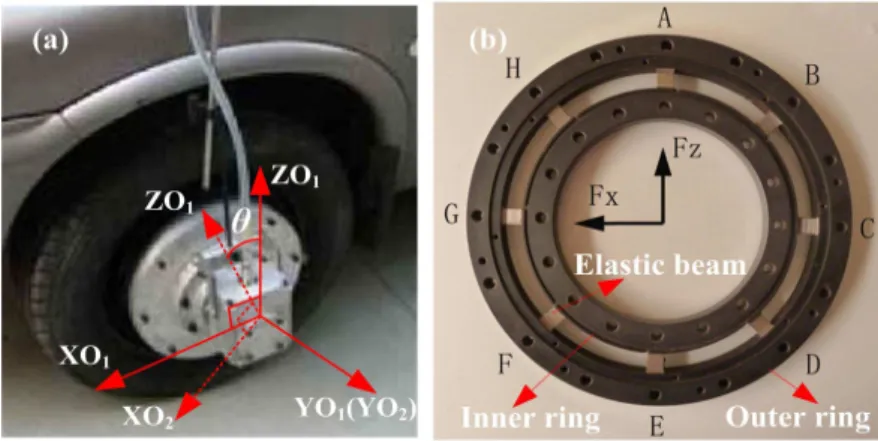
Generally, the multi-axis WFTs have quite similar systems consisting of the mechanical structures, data acquisition and signal transmission system such as the typical WFTs developed at Southeast University (Figure 1). Some design issues of WFT can be introduced for inertia coupling analysis.
Figure 1:Wheel/WFT coordinates systems (a) and the elastic body of the WFT (b) (developed at SEU refer to Lin et al., 2013; Lin et al., 2014; Chen et al., 2014).
2.1 Moving coordinate transformation
To apply a MFS to be the WFT in wheels, coordinate transformation exists between the spinning wheel and moving vehicle (see Figure 1(a)). When vehicle is moving, the vehicle Cartesian coordi-nate ( 0 - X Y Z1 1 1 1 ) can be transformed into wheel/WFT coordinate located in wheel center (0 - X Y Z2 2 2 2), the relation is given as
1 2
1 2
1 2
1 2
1 2
1 2
cos 0 sin 0 0 0
0 1 0 0 0 0
sin 0 cos 0 0 0
0 0 0 cos 0 sin
0 0 0 0 1 0
0 0 0 sin 0 cos
x x
y y
z z
x x
y y
z z
F F
F F
F F
M M
M M
M M
(1)
where is the rotating angle of the spinning wheel, subscript 1 and 2 represent the vehicle coordi-nates and the wheel coordicoordi-nates, respectively.
As a result of real-time periodic signal with the transfer matrix, the generalized wheel force/moment on the wheel can be measured and computed. More importance is that if considering
the wheel coordinate, all the deformations, stress and strain analysis can be carried out by the line-ar static method. Also the motion vectors as multi-axis accelerations of the WFT can be considered to be the static state, and therefore the equivalent mass or rotary inertia can be used in load distri-bution analysis of the WFT through Newton’s law of inertia.
2.2 Static structural analysis of the sensor
As the core part of a WFT, the elastic body structure (see Figure 1(b)) consists of eight elastic beams, one inner ring and one outer ring. Strain gauges are attached to the elastic beams which are used to sense deformation, and the two rings are used for force transmission between tyre and wheel hub, respectively. According to the theory of Material Mechanics, the hypothesis for stress-strain analysis can be listed essentially:
(1). Comparing to the small elastic beams, the two rings have large amount of mass and they will have the close fit joints attached to their connections (wheel hub or rim), so the two rings can be considered to be relatively rigid.
(2). In the process of elastic beams’ deformation, cross section perpendicular to the elastic beam keeps plane. Also no direct stress exists between the longitudinal fibers when shearing the beams.
Figure 2: The elastic beam and the deformations (Case.1 represents the tensile and compressive deformation; Case.2 represents the bending deformation; S1-S4 represent the strain gauges
and A-G represent the elastic beams, respectively).
To that extent, the boundary condition of the eight elastic beams will be fixed-end with only sup-ports shifting. That is, the inner ring is considered to be fixed and the outer ring has one free trans-lation degree at motion direction, or vice versa. When the six-axis forces are applied to the WFT individually, stress and deformation analysis can be given as below:
As is the case for a single force at X direction Fx, when it is applied to the WFT individually, beam C and G suffer the tensile and compressive deformations, respectively. Beam A and E are bending deformations, and the remaining beams B, D, F and H are combined deformations of ten-sile-compressive and bending, respectively. When a single force at Y direction Fy is applied to the
WFT, all the beams will produce bending deformations. The case of Fz will be the same as Fx
with 90 degrees rotation anticlockwise. Similarly, when a single moment Mx is applied, beams A and E are bending deformations, beams C and G are torsional deformations, and the remaining beams B, D, F and H are the combined deformation of bending and torsional deformations. When a single moment at Y direction My is applied, all beams produce bending deformations. The case of
z
M is similar to Mx as well.
According to the superposition principle in mechanics, the combined deformations can be de-composed into three basic deformation behaviors including tensile-compressive, bending, and tor-sional deformations. Since the measurement of tortor-sional deformation always needs a couple of strain gauges with 45 rotations with respect to the beam axis, we can just select tensile-compressive and bending deformations (See Figure 2). This makes all the strain gauges be of longitudinal arrange-ment along each elastic beam so that the torsional effect is removed.
Case.1. Tensile-compressive deformation (Figure 2(a)). In this case, the elastic beam forms the uniaxial stressed state and the stress relation is given as
x x
EA
F x A
l
(2)
where E is elastic modulus, x is the stress, l is the length of the beam and Abh is the cross
sectional area.
Case.2. Bending deformations (Figure 2(b)). A relative displacement occurs between the inner and outer ring, rotation and axial displacement are restricted by the rigid rings. The rotation-displacement formula of the structure is given as
2
3
6
12
AB BA
AB
EI
M z M
l EI
Q z
l
(3)
where MAB represents the bending moment, QAB represents the shearing force, and the I
3 12
bh is the geometrical moment of inertia.
Clearly, the stress is uniformly distributed along the beam in Case.1. But in Case.2, the anti-symmetric bending load makes an inflection point on the deformation curve so that only shearing force will exist and the bending moment is approximately zero; the maximum bending moment occurs at the end of beam.
Consequently, for measurement of bending deformation in Case.2, the strain-gauges can be ar-ranged at the end of each beam, and the beam’s side where neutral axis exists can be unoccupied. For measurement of tensile-compressive deformation in Case.1, discriminating measurement is taken into account so that the strain-gauges are arranged on neutral axis of each beam. Also, a finite ele-ment verification of the pure theoretical analysis was provided by us (Lin et al., 2014). However, the significance is that this detailed illustration not only gives the static strain and deformation analysis of the elastic body, but it will also be significant and applicable for the inertia load analysis of the transducer.
2.3 Self-decoupling approach and strain measurement
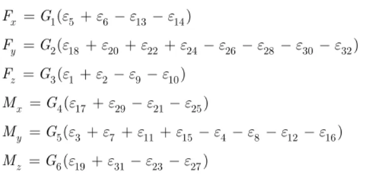
According to the strain and deformation analysis, bridge circuit can be built. Strain gauges on the elastic body are connected to one bridge per load component and total 32 strain gauges are hard-wired six full Wheatstone bridges, respectively (See Figure 3). Also temperature compensation will be achieved. Therefore, multi-dimensional outputs for the self-decoupled WFT is given by
F G
S or the form of1 5 6 13 14
2 18 20 22 24 26 28 30 32
3 1 2 9 10
4 17 29 21 25
5 3 7 11 15 4 8 12 16
6 19 31 23 27
( )
( )
( )
( )
( )
( )
x
y
z
x
y
z
F G F G F G
M G
M G
M G
(4)
where Gi represents the calibration coefficient for each individual load, i represents the output of
each strain gauge and
S is the strain output of the bridge. This determined connection modes ofthe bridge can completely eliminate the coupling interference between the six dimensions in theory, which means each applied force can affect only the output of the corresponding bridge while the outputs of the other bridges are irrelevant (Lin et al., 2014).
Figure 3: Strain-gauges arrangement (a) and the Wheatstone bridge connection mode. (b) The numbers of arrangement accord with that of Wheatstone bridge, representing strain gauges.
3 INERTIA INFLUENCE ANALYSIS FOR WFT
3.1 Inertia load distribution
To resolve the inertia influence on WFT, multi-axis accelerations can be investigated individually based on superposition principle. According to Newton’s law of inertia, the generalized inertia load is equivalent to the acceleration (or angular acceleration) multiplied by mass (or rotary inertia), so the inertia load distribution can be derived by static method. Since the inner ring of the elastic beam is considered to be a fixed-end, the outside parts such as the outer ring, rim, tyre and other mountings will be the effective inertia/mass.
(1). Inertia load at Y direction. As is the case for a single acceleration at Y direction ay, when it is applied to the WFT, an inertia force Fy can be uniformly distributed on eight elastic beams
with bending deformations. Each beam will have an extra output coupled into Fy signal with
= 8
y y i
F ma f
(5)
where m is the effective inertia-mass outside the elastic beams, i A, ..., H represent beam
num-ber. Similarly, when the angular acceleration at Y direction wy is applied individually, an inertia moment My is uniformly distributed with bending deformations. Replacing m with rotary inertia
y
J about Y axis, Eq. (5) can be the inertia load of angular acceleration at Y direction for each
beam.
(2). Inertia load at X or Z direction. When the acceleration ax is applied individually, the load distribution is
2 2 4
x x A C B
F ma f f f
(6)
where subscript A, B and C represent the beam number, respectively. The inertia load is distribut-ed with tensile-compressive deformations on beam C and G, bending deformations on A and E, combined deformations of tensile-compressive and bending on the remaining B, D, F and H beams, respectively. Therefore, the displacements can be given by Hooke's law as
3
3
12
2 24
A A
B B
B
C C
f l l
EI f l f l l
EA EI
f l l
EA
(7)
As the two rings are considered to be rigid body, beams A, B and C will have equivalent dis-placements at X direction with the compatibility equation as
A B C
l l l
(8)
Substituting the Eq. (6) and Eq. (7) into the Eq. (8), the inertia load distribution is obtained as
2 1 2
=
12 2 24
C A B x
Al Al
f f f ma
I I
(9)
where is the coefficient with respect to b, h and l.
The case of Fz will be same to Fx with 90 degrees rotation anticlockwise. Likewise, when the angular acceleration is applied individually, the inertia load can be given by replacing force F
with moment M. Using the same analytical method according to the above steps, inertia mo-ment distribution of Mz and Mx for each beam can be solved as well.
Until now, the inertial load distribution of the elastic body under multi-acceleration fields can be identified and calculated using the equations from Eq. (5) to Eq. (9). For each elastic beam, these inertia loads will produce extra strains in the outputs. According to Eq. (2) in Case.1 and Eq. (3) in Case.2, stress-strain and deformations of the inertial loads can be also easily calculated by the equa-tion of E.
3.2 Inertia decoupling output
Since the WFT is self-decoupled due to the strain gauge arrangement, inertia interference of elastic beams will be also reduced by the Wheatstone bridge to some extent. However, the remaining iner-tia errors may be transmitted and amplified by the calibration coefficient G because the calibration
is always performed under static condition. The model of multi-axis WFT with inertia decoupling can be obtained by rewriting Eq. (4) as
r o ine i ine i
F F f G
S
S K
S (10)where Fr is the true value of the wheel generalized force, Fo is the six output of WFT, fine is the inertia component which is coupled into the output, Ki is the modified calibration coefficient,
ine S
is the effective strain output of inertia component in theory which needs to be determinedin the following.
(1). Inertia coupled interference at Y direction. The inertia load Fy will have effect on all 32
strain gauges with bending deformations of each elastic beam, but only strain gauges (No. 17-24 and No. 24-32) on the dual surface of the beams have inertia components coupled into Fy output.
The remaining gauges could be easily compensated by bridge circuits (see Figure 3(b)). Therefore the extra strains which caused by inertia load in the output will have a total value of 8Fy with
2
0.5 3 8
Fy y y
Fy
t
F l ma l
E EW Ebh
(11)
where Wt 2I h is section modulus in bending, respectively.
Similarly, the inertia moment My will make the strains coupled on strain gauges No. 3, 4, 7,
8, 11, 12, 15 and 16 with a total value of 8My where
2
3 4
My y y My
J
E Ehb
(12)
(2). Inertia coupled interference at X or Z direction. In the case of inertia load Fx, different
deformations occur on beam C and G, beam A and E, and beam B, F, D and H, respectively. The deformations of beam A and E will have no influence on their strain gauges (No. 1, 2, 9, 10, 17, 21, 25 and 29) due to longitudinal or neutral axis arrangement. Though the combined deformation of tensile-compressive and bending occurs on beam B, F, D and H with strain gauges (No. 18, 20, 22, 24, 26, 28, 30, 32 and No. 3, 4, 7, 8, 11, 12, 15, 16), the coupled strains caused by inertia can be compensated by symmetrical structure and bridge circuits yet. Only the beam C and G with ten-sile-compressive deformations may have interference output on strain gauges of No. 5, 6, 19, 27, 13, 14, 23 and 31. According to Figure 3(b), the extra strain which caused by inertia load Fx is total of 4Fx where
=
Fx C x
Fx
f ma
E EA Ebh
(13)
Similarly, applying the same analysis procedure to the angular acceleration case, the extra strains which caused by inertia moment Mx will have effects on strain gauges No. 17, 25, 21, and 29. The result total value is 4Mx in which
2 Mx x x Mx
kJ E Ebh
(14)
The coefficient k is related to b, h, l and μ (the poisson ratio). Apparently, the inertia component for Fz and Mz will equal to Eq. (13) and Eq. (14) by replacing x with z, respectively.
If the motion information of three-axis accelerations and three-axis angular accelerations can be detected by such sensor units like six-axis MEMS sensors, the strain and deformation of the WFT under inertia loads will be easily calculated by Eq. (11) - Eq. (14). Substituting the strain values of inertia errors into the Eq. (10) and Eq. (4), the multi-axis wheel forces/moments with inertia de-coupling will be recorded in real time for the vehicle.
4 VERIFICATION AND EVALUATION
4.1 Numerical simulation using FEM
According to the theoretical analysis, inertial errors cannot be completely compensated by the strain gauge arrangements and Wheatstone bridges because the inertia loads make different defor-mation and strain output on the elastic body. Fortunately, the elastic body structure of the WFT can be resolved, formula deduction gives the inertia coupling mechanism under multi-axis accelera-tions. To test and verify the manual derivation, a set of parameters for the WFT can be given as: an 175/65-R14 tyre with the effective rolling radius of 284 mm, the total wheel mass of about
36 kg including 6.0 kg modified rim, 5.2 kg wheel hub, 10.03 kg tire and 14.52 kg WFT, etc. The
measured wheel rotational inertia Iy 1.88 kg·m2, Ix Iz0.92 kg·m2 where x, y and z represent
the rotation axis. The average maximum accelerations are about 4 m/s2 and 14.1 rad/s2 which cor-responding to the first gear for a passenger car. Calculated loads are approximate 150 N for the three inertia forces, 30 N·m for inertia moment at Y direction, and 15 N·m for inertia moment at X and Z direction, respectively. Applying the loads to the elastic body of WFT, finite element method (FEM) calculation can be performed.
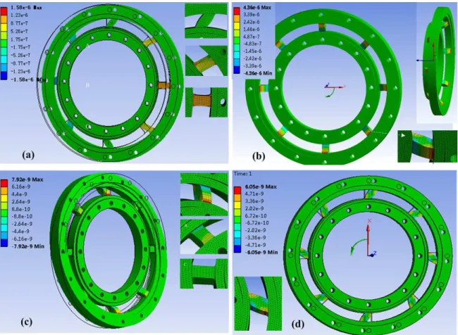
As shown in Figure 4, results indicate that the deformations and strain of elastic beam agree well with the analytical inertia load distribution. For inertia load Fx, the normal strain of beam C, B and A decrease in sequence at X direction. The maximum strain value occurs on beam C and G with tensile-compressive deformations while the strains on beam A and G with bending defor-mations are much small. For inertia load Fy, all the beams have same bending deformations with
the maximum value at the end of the beam. For inertia load My, all the beams have same
bend-ing deformations which are similar to the case of inertia load Fy. Likewise, for inertia load Mx, the normal strain of beam A, B and C decrease in sequence at X direction. A maximum strain value on beam A and E is observed while the beam C and G have much small strains. Detailed infor-mation of beam can refer to the inset figures in Figure 4 as well.
Figure 4: FEM results of inertia load for Fx (a), Fy (b), Mx (c) and My (d), respectively. Inset figures show the detailed information of deformation.
4.2 Evaluation of inertia coupling errors
By substituting the parameters into theoretical formulas and extracting the strains in FEM simula-tion, quantitative and comparative analysis of inertia coupling errors can be achieved. Table.1 shows the strain value under each inertia load individually (values at X and Z direction are equal). Also, the relative error between theoretical calculation and the FEM simulation can be defined as
100%
t s
s
v v r
v
(15)
where vt represents the values of theoretical derivation and vs represents the values of FEM
simu-lation.
Inertia load Fx(Fz) Fy Mx(Mz) My
Theoretical calculation (mm/mm) 1.21E-6 4.12E-6 6.95E-9 5.67E-9
Simulation result (mm/mm) 1.18E-6 4.25E-6 7.22E-9 5.85E-9
Errors (%) 2.5 3.1 3.7 3.1
Table 1: The strain values under inertia loads.
Results indicate that the strain values in FEM simulation agree well with that of the theoretical derivation for each inertia load. Since all the relative errors are less than 5%, within acceptable, it confirmed that the theoretical derivation is feasible. Although the errors exist, they are understand-able and foreseeunderstand-able not only because the hypothesis made a the pure theoretical derivation, but also due to chamfering geometric of structure, mesh quality of generation or other constraint rea-sons in simulation. Nevertheless, if considering a practical measurement range of 10000 N and
4000 N.m, the inertia loads will have the maximum impact on the signal output about 1.5%.
4.3 Experimental verification
To verify the inertia coupling errors, the WFT can be tested under six-axis acceleration fields. Due to the practical difficulties and economic reasons, the large six-axis acceleration simulation equip-ment is improbably built for us, but a three-axis self-decoupled WFT will be adequate for the nor-mal commercial vehicles (Lin et al., 2014). Therefore, the three-axis inertial load including Fx,
Fz and My will be verified herein. Besides, the linear acceleration test corresponding to Fx or Fz and the angular acceleration test corresponding to My will be designed into two different
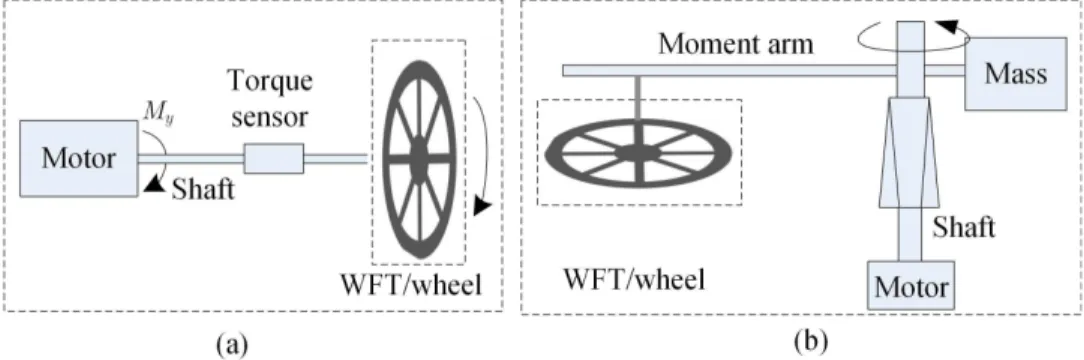
devices. For some reasons, details of the devices cannot be made public but a similar description can be seen in Figure 5. In both tests, the whole WFT is installed on wheel via bolts in the tests, so the WFT assembly can simulate real conditions.
For the inertial moment My under angular acceleration in Figure 5(a), a special tailored
de-vice containing a motor, a torque sensor and the assembled WFT is established. The motor applies the torque moment by controlling the accelerating time from zero to the rated angular velocity with a linear function generator, thus different angular accelerations are obtained. If being so, inertial
moment My can be applied to the WFT and can be fed back by a torque sensor of the motor.
For the inertia load Fx and Fz under linear acceleration, a geotechnical centrifuge (Ng et al.,
2001) is used to simulate the steady state acceleration field. Figure 5(b) shows its diagram where we see the WFT hanging below the moment arm. The centrifugal force is applied to the center of the WFT as the inertia load Fx or Fz.
Figure 5: The system diagram of the testing devices used for inertia coupling experiment. (a) The wheel inertia device used for My testing under angular acceleration; (b) The geotechnical centrifuge used for Fx and Fz
tests under linear acceleration.
Figure 6 shows that the wheel force output (longitudinal force Fx or vertical force Fz) and wheel
moment output (driving torque) are expressed as functions of the accelerations, respectively. It indi-cates that when the acceleration is increasing, the inertia load indeed have signal coupling output which can be detected by the sensor or WFT itself. The relationship between the applied accelera-tion and inertia load for both wheel force and moment is the approximate linear, respectively. Giv-ing an insight into the linear fittGiv-ing curves, the slopes represent the inertial-mass or rotational iner-tia of the wheel to some extent. The calculated values are 2.11 for ineriner-tia moment My, 351.2 for
inertia force Fx and 340.1 for inertia force Fz. The results are corresponding to the measured
rotational inertia of 1.88 kg.m2 and wheel mass of 36.0 kg. The deviation errors may result from the mass of the inner ring, the elastic beams of the elastic body, spindle of the test device or other parts which does not include in the WFT output. Besides, the deviation of inertia moment My between
torque-sensor-output and WFT-output is a little larger than the deviation of inertia force between
x F
WFT-output and Fz WFT-output. Because of different locations of the equipment in My
testing, the inertial mass for the torque sensor is a little larger than the inertial mass for WFT.
5 CONCLUSION
In conclusion, we have confirmed the inertia coupling characteristics induced from multi-axis accel-erations for the WFT. The inertial loads can be performed by the proposed theoretical approach which is verified by FEM analysis. Experimental verification is performed on the inertial loads Fx,
y
F
and My for the WFT as well. Several useful conclusions can be obtained as bellow:
(1) Though the proposed WFT is a self-decoupled, inertial loads cannot be compensated completely due to the structure and strain gauge arrangements.
(2) Inertia coupling mechanism of a WFT can be analyzed by the equivalent principle of inertia load, so that the inertia load distribution can be derived by static method.
Figure 6: Experimental results of inertial load. The signal outputs of inertial moment My (a) and that of inertial forces Fx and Fz (b) are expressed as functions of the accelerations, respectively. Curves are given as
polynomi-al fitting based on originpolynomi-al point data.
(3) From the aspect of structure analysis, the inertial errors can be calculated with manual deriva-tion. With the theoretical calculation, the equations may be coded into decoupling program in future signal processing and software algorithms for the real time output.
As the inertia loads have inevitable impact on the signal output, it will be of great significance for accuracy improvement of WFT. The generalized method and the derived formula in this paper not only give an insight into the inertia coupling mechanism of WFT, but also is used for correction of the calibration coefficient which obtained under static condition.
Acknowledgements
The authors would like to thank the anonymous reviewers for their useful comments and sugges-tions. The work was supported by Natural Science Foundation of China (51305078), Suzhou Science and Technology Project (SYG201303) and Funding of Jiangsu Innovation Program for Graduate Education (KYLX_0107).
References
Chen, X., Lin, G., Zhang, Y., (2014).Denoising method based on sparse representation for WFT. Journal of Sensors 145870.
Herrmann, M., Barz, D., Barber, J., (2005). An evaluation of the mechanical properties of wheel force sensors and their impact on to the data collected during different driving manoeuvres. SAE Technical Paper 2005-01-0857. Herrmann, M., Temkin, M., Black, L., (2006). The mechanical properties of wheel force sensors and their impact on to the data collected – a detailed consideration of specific tests. SAE Technical Paper 2006-01-0734.
Iombriller, S.F., Canale, A.C., (2001). Analysis of emergency braking performance with particular consideration of temperature effects on brakes. Revista Brasileira de Ciencias Mecanicas/Journal of the Brazilian Society of Mechani-cal Sciences 23(1): 79-90.
Kim, J.H., Kang, D.I., Shin, H.H., Park, Y.K., (2003). Design and analysis of a column type multi-component force/moment sensor. Measurement 33(3): 213-219.
Lin, G., Zhang, W., Yang, F., Pang, H., Wang, D., (2013). An initial value calibration method for the wheel force transducer based on memetic optimization framework. Mathematical Problems in Engineering, 275060.
Lin, G.Y., Pang, H., Zhang, W.G., Wang, D., Feng, L.H., (2014). A self-decoupled three-axis force sensor for measur-ing the wheel force. Proceedmeasur-ings of the Institution of Mechanical Engineers-Part D: Journal of Automobile Engineer-ing 228(3): 319-334.
Liu, S.A., Tzo, H. L., (2002). A novel six-component force sensor of good measurement isotropy and sensitivities. Sensors and Actuators A: Physical 100(2): 23-230.
Ma, J., Song, A., Pan, D., (2013). Dynamic compensation for two-axis robot wrist force sensors. Journal of Sensors 357396.
Mokhiamar, O., Abe, M., (2002). Active wheel steering and yaw moment control combination to maximize stability as well as vehicle responsiveness during quick lane change for active vehicle handling safety. Proceedings of the Insti-tution of Mechanical Engineers-Part D: Journal of Automobile Engineering 216(2): 115-124.
Ng, C., Van, L.P., Tang, W.H., Li, X.S., Zhang, L.M., (2001). The Hong Kong geotechnical centrifuge. Proceedings of the 3rd international conference soft soil engineering, Hong Kong, pp. 225-230.
Pavkovic, D., Deur, J., Hrovat, D., Burgio, G., (2009). A switching traction control strategy based on tire force feedback. IEEE conference on control applications and intelligent control, Saint Petersburg (Russia) 8: 588-593. Song, A.G., Wu, J., Qin, G., (2007). A novel self-decoupled four degree of freedom wrist force/torque sensor. Meas-urement 40(9): 883-891.
Weiblen, W., Kockelmann, H., Burkard, H., (1999). Evaluation of different designs of wheel force transducers (part II). SAE Technical Paper 1999-01-1037.
Wu, B., Shen, F., Ren, Y., (2011a). Development of an integrated large range six-axis force sensor for centrifuge test in acceleration field. Journal of Astronautics 32(9): 2080-2087.
Wu, B., Luo, J., Shen, F., Ren, Y., Wu, Z. (2011b). Optimum design method of multi-axis force sensor integrated in humanoid robot foot system. Measurement 44(9): 1651-1660.
You, S.S., (2012). Effect of added mass of spindle wheel force transducer on vehicle dynamic response. SAE Tech-nical Paper 2012-01-0210.
Zhang, L., Liu, H., Zhang, H., Xu, Y., (2011). Component load predication from wheel force transducer measure-ments. SAE Technical Paper 2011-01-0737.
Zhang, X.L., Li, L., Jiang, S., Cao, C.M. (2012). Effect of wheel force transducer’s mass on measurement precision and whole vehicle stability (in Chinese). Journal of Mechanical Engineering 48(22): 121-126.