Abstract
Pneumatic isolators are promising candidates for increasing the quality of accurate instruments. For this purpose, higher perfor-mance of such isolators is a prerequisite. In particular, the time-delay due to the air transmission is an inherent issue with pneu-matic systems, which needs to be overcome using modern control methods. In this paper an adaptive fuzzy sliding mode controller is proposed to improve the performance of a pneumatic isolator in the low frequency range, i.e., where the passive techniques have obvious shortcomings. The main idea is to combine the adaptive fuzzy controller with adaptive predictor as a new time delay con-trol technique. The adaptive fuzzy sliding mode concon-trol and the adaptive fuzzy predictor help to circumvent the input delay and nonlinearities in such isolators. The main advantage of the pro-posed method is that the closed-loop system stability is guaran-teed under certain conditions. Simulation results reveal the effec-tiveness of the proposed method, compared with other existing time –delay control methods.
Keywords
Pneumatic vibration isolation; transmissibility; AFSMC; input delay; uncertain dynamic system.
Control of input delayed pneumatic vibration isolation table
using adaptive fuzzy sliding mode
1 INTRODUCTION
Pneumatic vibration isolators (PVIs) are simple and effective vibration isolators. The vibration-sensitive equipment can be isolated using PVIs; for example, for the wafer scanners to fabricate integrated circuits, and the electron microscopes used for submicron imaging (Subrahmanyan and Trumper, 2000). PVIs isolate the vibration properly in the frequency range above the resonance frequencies associated with larger masses with a small stiffness characteristic (Heertjes and van de Wouw, 2006). Due to more precise measurement requirements and the sensitivity of the equipment to vibration, the standards for ground vibration in the frequency range lower than 10 Hz have be-come tougher (Gordon, 1999). The simultaneous vibration reduction at excitation frequencies above
Mostafa Khazaeea* Amir H.D. Markazib
a,bDigital Control Lab., School of Mechanical Engineering, Iran University of Science and Technology, Narmak, 16846, Tehran, Iran
Corresponding author: a*[email protected]
http://dx.doi.org/10.1590/1679-78251646
and below the system natural frequencies, which are typically 2-6 Hz, is a hard design constraint. Therefore, the active control of the pneumatic vibration isolation tables was considered as an effec-tive vibration reduction way for the low excitation frequencies (Shin and Kim, 2009).
Previous works on active control of vibration isolators are often based on linear control tech-niques (Beard et al., 1994; Nagaya and Kanai, 1995). An active/passive nonlinear isolator was pro-posed which used some optimization techniques (Royston and Singh, 1996). PVI control by combin-ing feedback linearization with a linear loop-shapcombin-ing controller is adopted (Heertjes and van de Wouw, 2006). The mentioned active control techniques need the measurement of acceleration and not the pressure or mass flow rate (Chen and Shih, 2007). The compensation of the pneumatic iso-lation table fluctuation which is caused by switching of the feedforward compensator was considered (Shirani et al., 2012). These control methods cannot suppress both the seismic vibration and the direct (payload) disturbances simultaneously. A state space representation of PVIs and a robust time delay control design was presented (Chang et al., 2010). This control algorithm achieved the suppression of seismic vibration and payload disturbance. Many of the existing methods heavily rely on the mathematical model of the plant, while the model of a typical PVI contains many uncertain-ties and nonlineariuncertain-ties. Therefore, many of such methods cannot guarantee the closed-loop stability under real situations.
In this paper, the adaptive fuzzy sliding mode controller (AFSMC) (Poursamad and Markazi, 2009) is used for the purpose of controlling PVIs. A fuzzy system estimates an ideal sliding-mode controller, and a switching robust controller compensates for the difference between the ideal con-troller and the fuzzy approximation. The parameters of the fuzzy system and the uncertainty bound of the robust controller, are tuned adaptively. Furthermore, a predictor estimates the future value of the sliding surface parameter. The fuzzy system and adaptive rules use the prediction error to minimize the difference between the estimated value and the actual one in the prediction horizon. The predictor is designed by a one-step-ahead algorithm which reduces the computational cost sig-nificantly.
Through this adaptive control algorithm there is no need for known uncertainty bounds of the pneumatic vibration isolator table model, as long as the bound exists. Also, the sliding mode scheme compensates for the uncertainties and disturbances by means of controlling the pressure inside the pneumatic chamber.
The outline of this paper is as follows. ‘Problem statement and preliminaries’ are provided in Section 2. Section 3 introduces the controller and predictor and investigates the closed-loop stabil-ity. Evaluation of the proposed method is considered in Section 4, by simulation studies and com-parison to the results of the Time-delay control method introduced in (Shin and Kim, 2009). Con-cluding Remarks are given in Section 5.
2 PROBLEM STATEMENT AND PRELIMINARIES
2.1 Mathematical modeling of the PVIT
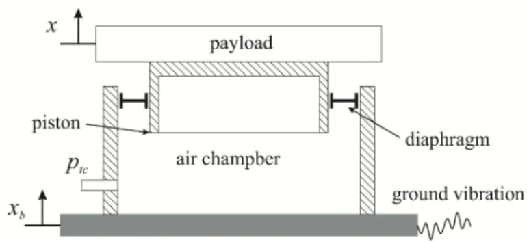
Consider a pneumatic vibration isolation system consisting of a payload and a single pneumatic chamber as shown in Figure 1. Stiffness of the single chamber is known to be dependent on frequen-cy and amplitude of vibration (Lee and Kim, 2007).
Figure 1: Pneumatic table for isolation of equipment from excitation at ground.
The governing equation for the mentioned pneumatic vibration isolation table can be written in the state space form as
00 1 0
1 s d b d b p tc
s d d
x x
k k x c x A p
k k c
x x
m
m m m
, (1)
where, x x x is the state vector which consists of the payload vertical movement and velocity. The payload is attached to the base by means of PVI, but the table is disturbed by the base movement xb xb xb, so the second term in the right hand side of (1) represent the ground vibration effects.ptc is the dynamic pressure from the actuator as the control input of system. Also,
m denotes the mass of payload, ks p A0 p2 /Vt0 real stiffness of the single chamber, kd and cd is real part of the complex stiffness of diaphragm and equivalent viscous damping of diaphragm, re-spectively. Ap is the effective area of the piston cross-sectional area and the diaphragm (Shin and
Kim, 2009; Lee and Kim, 2007). Table 1 gives the values of the parameters of mentioned system. It should be noted here that the actuators and sensors which is used for controlling such systems, have some time delays (Chang et al., 2010). This problem gets more importance when high precision of the installed equipment on PVIT is required. Therefore, it is considered that ptc reaches the plant with a time delay , as a common way for modeling of the mentioned actuation and measurement delays (Galambos et al., 2014).
Symbol Name Value
m Payload 87 kg
Specific heat ratio 1.4
0
p Static pressure 3.51×10⁵ Pa
0 t
V Chamber volume 2.978×10⁻⁴ m3
p
A Effective piston area 2.518×10⁻³ m2
d
c Equivalent viscous damping of diaphragm 2.78×10² N.s/m
d
k Real part of complex stiffness of diaphragm 1.12×10⁴ N.s/m
Table 1: Parameters of pneumatic spring and payload.
2.2 General problem statement
For the time delay control of PVIs, the general problem can be considered as the following input-delayed nonlinear system as
nx t f g u t
y t C
x x
x (2)
where x x x1, ,1,xnT n, y t
and u t
are the system states, measurable outputand input, respectively, f
and g
are probably unknown but smooth nonlinear functions, and is a constant delay. The control goal is that u t
causes the system tracks a desired state vector
d tx and closed-loop signals remain bounded. It is mentioned that the proposed control design
method can be used for nonlinear affine-in-control systems and it is not limited to the SISO sys-tems.
For the adaptive fuzzy sliding mode control (AFSMC) in contrast with time delay control tech-niques (TDC) (Heertjes and van de Wouw, 2006; Shin and Kim, 2009; Lee and Kim, 2007), there is no need for precise model and the availability of all states. In the so called TDC techniques the delayed value of dynamics f
x,t
and g
x,t
are used to approximate the control signal
u t , where is an overall time delay. Thus, the input time delay must be considered for
control-ling the PVIs, and the control problem is changed to an input delay system. The proposed AFSMC with adaptive fuzzy predictor which are introduced in the next section, can enhance the perfor-mance of PVIs by solving this control problem.
In this paper, the following single output linear parameter fuzzy system is employed to approxi-mate the nonlinear function and input signal over a compact set X with input x x1 xn, and nr IF-THEN rules; for example,
Rule r : IF x1 is A1r and … and xn is Anr THEN f
x kr, r 1, ,nr,where f is the output of the fuzzy system, kr is the fuzzy singleton for output of rth rule, and
1r, , nr
A A are the fuzzy sets defined through some Gaussian membership functions as
2 exp r j r j j j A r j x c x (3)in which r j
c and rj are the center and width of the Gaussian membership function. Define the fir-ing strength of the rth rule as
1 1 1 i r j r i r i n j A jr n n
i A i r x w x
(4)and using singleton fuzzification, product inference system, and center average deffuzification, the output of the fuzzy algorithms yield as
*T
, nf x k w x x X (5)
where * * *
1, , r r
T n
n
k k
k is the bounded vector of output fuzzy singleton and is a bounded error, i.e., *
N
k k , N with kN and N being positive constants. w x
1 , , r
T n
w w
x x is the vectors of firing strength of rules.
Remark 1. The fuzzy system (5) uniformly approximates f X: Y if X is compact (closed and
bounded) and f is continuous. Then, the approximation error uniformly converges to zero, thus
is a bounded error (Kosko, 1994).
3 PREDICTOR AND CONTROLLER DESIGN
3.1 Adaptive Fuzzy Predictor (AFP)
The first step is developing an adaptive predictor for system (2). Select positive parameters a1,...,an an appropriately such that the polynomial 1
1 ...
n n
n
s a s a is Hurwitz, then the following
ma-trix A is stable and select the symmetric positive definite matrices P and Q such that the
Lya-punov matrix equations A PT PA Q and PB CT are satisfied.
1 2 3
0 1 0 0 0 1
0 0 1 0 0 1
, ,
0 0 0 1 0 1
1 1
T
n
A B C
a a a a
(6)
The unknown nonlinear functions f
x and g
x can be approximated using the fuzzy systemswith input xˆ
t , the predictor state vector. According to (5), the output of fuzzy algorithms yieldas
* f T
fuz f
f h w (7)
* g T
fuz g
g q w (8)
over a compact set, where [ ,1 , ]
r T m
h h
h and [ ,1 , ]
r T m
q q
q are the vectors of output fuzzy singleton, [ 1, , ]
r T f wf wfm
w and [ 1, , ]
r T g wg wgm
w are the vectors of firing strength of rules. The nonlinear system (2) with input delay, can be considered as follows
1 ; 1, , 1
i i
n
x t x i n
x t f g u t
y C x x x (9)
where 1, ,1 , T n
n x x x
x is the state vector of system (2).
Regarding the fact that the fuzzy output vectors h and q contain the behavior of system dynam-ics, the following online predictor can be designed by appropriate adaptation algorithm.
| | | | | ˆ |ˆT T
p p f g
p p
t t A t t B t t t t u t
y t t C t t
x x h w q w
x
(10)
where xp
t |t
x1p
t |t
,,xn p
t |t
n and yp
t |t
are thepredic-tions of the future system states and output of (9) respectively. The following adaptation algorithm is employed to update the fuzzy output vectors
1 1
2 2
| | | |
ˆ | | |
ˆ ˆ
ˆ |
p f
p g
t t y t t t t t t
t t y t t t t t t
w h
q w q
h
(11)
where T 0, 1, 2
i i i
are adaptation rates, i 0 are modification parameters, and
p p
y y y is the predictor output error.
The prediction error dynamics is obtained by subtracting (10) from (9) as
|
p t t p t t
x x x (12)
| |
T
p p f g
p p
t A t B t t t t u t
y t C t
x x h w q w
x
(13)
where approximation and the overall error h, q, and are defined as
* ˆ
h h h (14)
* ˆ
q q q (15)
*T | *T |
f t f t t f g t g t t g u t
h w w q w w (16)
Remark 2.It is stated that the fuzzy estimation error is bounded and converges to zero in Remark (1), i.e., f and g are bounded. The optimum values of fuzzy inputs are not infinity, thus, h* and
*
q are bounded. Also, w
is bounded based on the definition in (4). Finally, it is concluded that is a bounded error. So that N holds with N being a positive constant. Then the following lemma is achieved.
Lemma 1. Consider nonlinear system (2), the adaptive fuzzy predictor is given in (10) with the adaptive law (11), then the predictor error xp and the fuzzy output vector errors h and q are
uniformly ultimately bounded.
Proof. Select the Lyapunov candidate function for predictor as
1 2
1 1 1
, ,
2 2 2
T T T
p p p p
V t P
x h q x x h h q q (17)
1 2
1 1 1
| |
2
T T T T T
p p p p f g
V Q y t t t t u t
x x h w q w h h q q
From the predictor adaptation algorithm (11) it can be concluded that
1 2
1 2
T T T
p p p p
V Q y
x x h h q q
By using Young’s inequality
2 2 2
1 2 1
b a k b k , k1 0
1 2
1
1
2 2
p p N
k y
k x
*
1 1 *2 , h, q2 2
ˆ
T T
i i i i i i i i
K K K K K K K K
1 2 1 *2 2 *2 21 1 1
1
1 1
2 2 2 2 2 2
p m p N p
V Q k V
k
x h q h q
11 min , 1 1, 2 2 0
m m Q k P
and const.
*2 *2 2
1 1 2
1
1 1
0
2 k N
h q
After selecting the appropriate parameters for the predictor, it can be shown that 1Vp 1 0 for all xp
t within a compact set Xp, then the time derivative of Lyapunov function of predictoris negative semi-definite. Also, because the input delay does not affect the stability proof of predic-tor, there is no need to use the stability analysis for time-varying system for it. Thus, xp and the
fuzzy output vector errors h and q are uniformly ultimately bounded.
3.2 Adaptive Fuzzy Sliding Mode Controller (AFSMC)
The prediction of future system states xp
t |t
are derived based on the current systeminfor-mation from predictor (10). Now, sliding mode control based on states xp
t |t
compensatesthe effect of input delay in the feedback loop. In this section, a sliding mode feedback control is designed for tracking of reference signal and the overall closed-loop stability.
Consider the fuzzy systems with input s tˆ
|t
, which is obtained as
1
| |
ˆ n
s t t D x t t (18)
t |t
d
t
p
t |t
x x x
(19)
where x
t |t
is the predicted value of x
t . Based on (5) we haveT fuz
u k w (20)
where 1, ,
r T n
k k
k is the vector of output fuzzy singleton, and 1, ,
r T n
w w
w is the vector
of firing strength of rules. The estimation error of the fuzzy system is denoted by which is assumed to be bounded, i.e.,
(21)
where is estimation error bound. An adaptive algorithm is used for tuning the fuzzy singleton output as
1 | sgn
ˆ s tˆ t g
k k w (22)
where 1 is adaptation rate and kˆ is the estimated value of output fuzzy singleton, and
ˆ
k k k (23)
Therefore, the output of fuzzy system can be rewritten as
ˆ ˆfuz T
u k w (24)
To compensate the fuzzy estimation error, the urb is designed as
s ˆ sg
ˆ gn | n
rb
u s t t g (25)
where ˆ is the error bound estimation which is adjusted adaptively by
2
ˆ s tˆ |t
(26)
where 2 is a positive constant which is defined by designer and
ˆ
(27)
The total control signal consist of both fuzzy and robust control as
ˆfuz rb
u u u (28)
Lemma 2. Consider nonlinear time-delay system (2), the predictor (10) with the update law (11)
and the adaptive fuzzy sliding mode controller (28) with the adaptive law (22) and (26), then (1) All signals in the closed-loop system are bounded.
(2) The tracking error x and the fuzzy estimation errors k and are uniformly ultimately
bound-ed.
Proof. Select the Lyapunov candidate function for the controller as
2 2
1 2
1
2 2 2
T c
g g
V s
k k (29)
For delay compensation the sliding surface is constructed as shown in (18). Remembering that the final goal is to make actual sliding surface of system zero,
n 1
s t D x t (30)
and
d
x t x t x t (31)
From (2), (28), (30), and (31) the derivative of sliding surface derived as
1
1 *
1
,
ˆ kˆ ,ˆ
n
n n n i i
i fuz rb
i
s D C D x g u u s u s
x
(32)
The time derivative of Lyapunov function (29) is
1 2
1
sgn .
T
c rb
g
V g s g s g u
k w k
.
By using (22), (26), and (28) in the derivative we have
ˆ |
ˆsgn ˆ
|
ˆ
|
T c
V sggk w ss t t s g s t t g s t t (33)
Based on Lemma 1, the predictor error will be bounded as last, thus
0 0
lim p 0 lim p |
t t t t t t
x x x
By using the later result and (18), (19), (30), and (31) it concluded that
0im ˆ |
l
ts t s t t
(34)
Based on the results of (33) and (34), the derivative is simplified as
ˆ ˆ .
c
V sg s g g s s g s g s g s g
0c
V s g
(35)
c
V is semi-negative definite then the system is stable and s, k, and will remain bounded. Now
consider the following Lipchitz function
t s g
VC (36)
From integrating
t it can be shown that
0
d 0 , , , ,
t
C C
V s V s t
k k because VC
s
0 , ,k
is bounded and VC
s t
, ,k
is non-increasing and bounded, therefore
0lim d
t
t
also, by using the Barbalat Lemma, it is concluded that lim
0t t and limts t
0. Finally it isproved that all signals in the closed loop system will remain bounded and the tracking error is uni-formly ultimately bounded.
4 SIMULATION STUDY
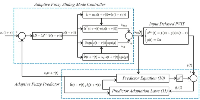
The proposed AFSMC-AFP consists of a predictor (10) and a sliding mode controller (28). Figure 2 depicts the block diagram of the control algorithm for the general form of Pneumatic Vibration Isolation Tables (PVITs). The simulation is done by using the control algorithm for the system (1), where u t
ptc is input signal. The control command is sent to an electrical drive board whichprovides the reference voltage for the control servo valve, a proportional valve of nozzle-flapper type (Chang et al., 2010). The valve regulates the dynamic pressure of the chamber. But this actuation process causes an input time delay 0.01 s.
In order to apply the AFSMC, the desired state vector is xd
t 0 and the sliding surface is defined ass x x (37)
In the simulation, the input membership functions are Gaussian. The initial fuzzy output vector are arbitrarily to select as kˆ 0.5 0 0.5T and the initial value of uncertainty bound is chosen as
ˆ 0.05
. The adaptation rate are set to 1 0.1 and 2 1. The predictor parameters are se-lected as a1 5, a2 5, and the learning gains are specified as 1 50 and 1 0.05. It is
not-ed that the adaptation rate can be tunnot-ed basnot-ed on the size of delay to achieve the good perfor-mance.
Figure 2: Schematic diagram for proposed AFSMC-AFP.
In this study, a random ground vibration with rate of xb 30mm/srms is used as the base
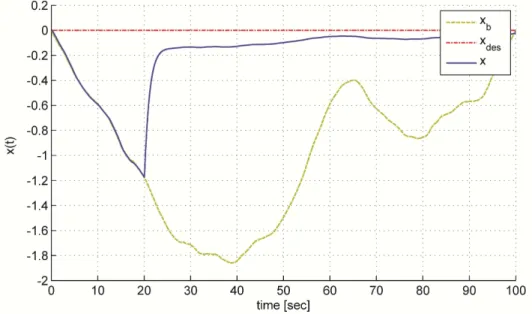
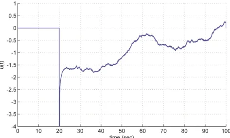
excita-tion. This excitation is the criteria VC-C in standard of ground vibration (Gordon, 1999) and is allowed marginally for electron microscopes. The system parameters are as in Table 1 for the simu-lation. The time responses of system are presented in Figures 3 and 4, and the control signal in Figure 5. It is noted that the AFSMC-AFP starts at t 20 s for better understanding. The ratio
of cross-and auto- correlation of the vibration signals at the payload is a common index for deter-mining the isolation performance. This index is called transmissibility which is estimated from the two signals as follows
BX BB G Transmissibility
G
(38)
where the subscripts B and X denote the vibration signals at the base and on the payload, respec-tively, GBX and GBB cross- and auto-power spectral density function, respectively. For the calcula-tion of this index Hanning window is applied by ensemble average of 50 times, and at a frequency resolution of 0.2 Hz. Figure 6 shows the transmissibility index and isolation performance by the AFSMC-AFP can be better than the TDC technique and the passive one. The root mean square of the transmissibilities by the AFSMC-AFP is less than 40 % of TDC and 2 % of that by the passive one in the frequency range under 7 Hz which is very desirable for enhancing the vibration isolation performance of table for low frequency around the resonance.
Simultaneous suppression was analyzed with seismic vibration and direct disturbance being ap-plied to system. The seismic disturbance was generated in the same way as before, but this time a direct disturbance is applied at t 20 s. Figure 7 shows the time response of the payload resulting
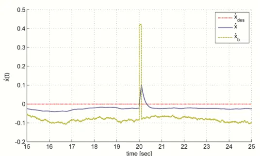
passive PVI (3.10 s) and less than 50% of TDC (0.99 s). So that based on these results it is evident that the AFSMC-AFP is an effective control scheme for PVIT in simultaneous suppression.
Figure 3: Normalized System position response to seismic vibration VC-C ground vibration ( 0.01s).
Figure 4: Normalized System velocity response to seismic vibration VC-C ground vibration (0.01s).
Frequency Range Passive TDC AFSMC
Root means square (RMS) 1 – 10 Hz 2.8345 0.1291 0.0469
10 – 30 Hz 0.0445 0.0618 0.1948
Table 2: RMS value of transmissibility magnitude.
Figure 5: Normalized AFSMC-AFP control signal for seismic vibration VC-C ground vibration (0.01s).
Figure 6: Transmissibility of passive, active, and AFSMC controlled pneumatic vibration table in presence of VC-C ground vibration ( 0.01s).
5 CONCLUSION
In this paper, a new method of adaptive active control is proposed for the pneumatic vibration iso-lation tables. As the ground isoiso-lation requirements of vibration sensitive equipment become more stringent, the active control of such devices are unavoidable. In the previous sections it is shown that the proposed adaptive fuzzy sliding mode control with adaptive fuzzy predictor can handle this problem in a good way. This method does not require the precise model and magnitude of the un-certainties. Also, the linearity or nonlinearity of model is not important. AFSMC design results in the desired low-amplitude response, thus attaining a higher isolator performance.
Figure 7: Normalized System velocity response to seismic vibration and direct disturbance at t = 20 s.
References
Beard, A., Schubert, D., von Flotow, A., (1994). Practical product implementation of an active/passive vibration isolation system. SPIE's 1994 International Symposium on Optics, Imaging, and Instrumentation, pp. 38-49.
Chang, P.-H., Ki Han, D., Shin, Y.-H., Kim, K.-J., (2010). Effective suppression of pneumatic vibration isolators by using input--output linearization and time delay control. Journal of Sound and Vibration 42(5): 1636-1652.
Chen, P.C., Shih, M.C., (2007). Modeling and robust active control of a pneumatic vibration isolator. Journal of Vibration and Control 13(11): 1553-1571.
Galambos, P., Baranyi, P., Arz, G., (2014). Tensor product model transformation-based control design for force reflecting tele-grasping under time delay. Proceedings of the Institution of Mechanical Engineers, Part C: Journal of Mechanical Engineering Science 228: 765-777. SAGE Publications.
Gordon, C., (1999). Generic vibration criteria for vibration-sensitive equipment. SPIE's International Symposium on Optical Science, Engineering, and Instrumentation, pp. 22-33.
Heertjes, M., van de Wouw, N., (2006). Nonlinear dynamics and control of a pneumatic vibration isolator. Journal of Vibration and acoustics 128(4): 439-448.
Kosko, B., (1994). Fuzzy systems as universal approximators. IEEE Transactions on Computers 43(11): 1329-1333. Lee, J.-H., Kim, K.-J., (2007). Modeling of nonlinear complex stiffness of dual-chamber pneumatic spring for preci-sion vibration isolations. Journal of sound and vibration 301(3): 909-926.
Nagaya, K., Kanai, H., (1995). Direct disturbance cancellation with an optimal regulator for a vibration isolation system with friction. Journal of sound and vibration 180(4): 645-655.
Poursamad, A., Markazi, A. (2009). Adaptive fuzzy sliding-mode control for multi-input multi-output chaotic sys-tems. Chaos, Solitons & Fractals 42(5): 3100-3109.
Royston, T., Singh, R., (1996). Optimization of passive and active non-linear vibration mounting systems based on vibratory power transmission. Journal of Sound and Vibration 194: 295-316.
Shin, Y.-H., Kim, K.-J., (2009). Performance enhancement of pneumatic vibration isolation tables in low frequency range by time delay control. Journal of Sound and Vibration 321(3): 537-553.
Shirani, H., Nakamura, Y., Wakui, S., (2012). Control of a pneumatic isolation table by flow meter: Improvement of repeatability in various switching points of the feedforward compensator. Advanced Mechatronic Systems (ICAMechS), 2012 International Conference on (pp. 609-614). IEEE.
Subrahmanyan, P., Trumper, D., (2000). Synthesis of passive vibration isolation mounts for machine tools a control systems paradigm. American Control Conference, 2000. Proceedings of the 2000. 4, pp. 2886-2891. IEEE.