Adv. Sci. Res., 7, 11–20, 2011 www.adv-sci-res.net/7/11/2011/ doi:10.5194/asr-7-11-2011
©Author(s) 2011. CC Attribution 3.0 License.
Advances
in
Science & Research
Open Access ProceedingsTWINN
Results
–
Chapter
2
Regional climate projections in two alpine river basins:
Upper Danube and Upper Brahmaputra
A. Dobler1, M. Yaoming2, N. Sharma3, S. Kienberger4, and B. Ahrens1
1Institute for Atmospheric and Environmental Sciences, Goethe University, Frankfurt am Main, Germany 2Institute of Tibetan Plateau Research, Chinese Academy of Sciences, Beijing, China
3Department of Water Resources Development & Management, Indian Institute of Technology, Roorkee, India 4Centre for Geoinformatics, University of Salzburg, Austria
Abstract. Projections from coarse-grid global circulation models are not suitable for regional estimates of water balance or trends of extreme precipitation and temperature, especially not in complex terrain. Thus, downscaling of global to regionally resolved projections is necessary to provide input to integrated water resources management approaches for river basins like the Upper Danube River Basin (UDRB) and the Upper Brahmaputra River Basin (UBRB).
This paper discusses the application of the regional climate model COSMO-CLM as a dynamical downscaling tool. To provide accurate data the COSMO-CLM model output was post-processed by statistical means. This downscaling chain performs well in the baseline period 1971 to 2000. However, COSMO-CLM performs better in the UDRB than in the UBRB because of a longer application experience and a less complex climate in Europe.
Different climate change scenarios were downscaled for the time period 1960–2100. The projections show an increase of temperature in both basins and for all seasons. The values are generally higher in the UBRB with the highest values occurring in the region of the Tibetan Plateau. Annual precipitation shows no substantial change. However, seasonal amounts show clear trends, for instance an increasing amount of spring precipitation in the UDRB. Again, the largest trends for different precipitation statistics are projected in the region of the Tibetan Plateau. Here, the projections show up to 50% longer dry periods in the months June to September with a simultaneous increase of about 10% for the maximum amount of precipitation on five consecutive days. For the Assam region in India, the projections also show an increase of 25% in the number of consecutive dry days during the monsoon season leading to prolonged monsoon breaks.
1 Introduction and objectives
The Danube and the Brahmaputra River have their headwa-ters in mountainous regions where massive glacier retreat and permafrost thaw have been observed in recent times. Thus, further climate warming is likely to impact water availabil-ity and hydrological dynamics in both river-basins. In this regard climate model projections can be used to gain some estimate of possible future impacts.
To estimate the impact of future climate change on the hy-drology at the basin scale, climate projections with a suitable temporal and spatial resolution are essential input to hydro-logical models. However, projections from current global circulation models (GCMs) have a grid resolution of about
Correspondence to:A. Dobler ([email protected])
200 km or more. Further, these projections mostly agree on the global and continental scale of precipitation and tempera-ture change in the 21st century, but the projections for precip-itation changes diverge with decreasing spatial scales (Bates et al., 2008).
Thus, GCM projections are inappropriate to assess the im-pact of climate change on a regional scale related to inte-grated water resources management (IWRM) in the UDRB and the UBRB. A downscaling of the large-scale simulations to a resolution of 50 km or less is necessary (Ahrens, 2003; Beck et al., 2004; Frei et al., 2003; Salath´e, 2003). To this end, it is essential to find a well suited GCM and to apply an appropriate downscaling method to the GCM projections.
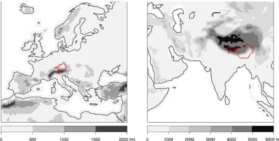
Figure 1.Model orography used in the European (left) and the South Asian (right) computational domain with the UDRB and the UBRB, respectively.
2 Role within the integrated project
As glacier and permafrost melting are natural system pro-cesses with long response times, the respective impact mod-els should be driven by transient regional climate projec-tions. However, due to limited available computational power, there has been a lack of transient projections, espe-cially in South-Asia where earlier studies (e.g., Kumar et al., 2006) mostly were based on time slice experiments.
Within the BRAHMATWINN project (http: //www.brahmatwinn.uni-jena.de) downscaled GCM pro-jections were used as input to the hydrological model DANUBIA to simulate historical and future water balances of the UDRB and the UBRB (Prasch et al., 2011). Further-more the data were used in snow glacier and permafrost modelling (Lang et al., 2011) and, to assess the question of a changing climate directly, in the calculation of climate change indicators (Giannini et al., 2011a, b).
To cope with these necessities, we provided transient cli-mate projections for the UDRB and the UBRB covering the years 1960–2100. The scenarios A1B, B1, A2, and the com-mitment scenario, as given in the IPCC Special Report on Emissions Scenarios (SRES, Nakicenovic and Swart, 2000), were used to generate a small ensemble of possible future developments.
3 Scientific methods applied
The testing and further development of existing downscaling techniques is an important first step in the generation of re-gional climate projections with a high temporal and spatial resolution. The latter is a prerequisite to evaluate the use of these data for the estimation of the regional impact of future climate change.
Generally, two different classes of downscaling methods may be applied (Murphy, 1999; Xu, 1999): (a) dynami-cal downsdynami-caling methods based on simulations of physidynami-cal processes at a fine scale, typically using a regional climate model (RCM) and (b) statistical downscaling methods that employ observed statistical relationships between the coarse and the fine scale. Dobler and Ahrens (2008) tested diff er-ent statistical, dynamical and combined downscaling meth-ods on global ERA-40 re-analysis data (Uppala et al., 2005) in Europe and South Asia with respect to rain day frequency and intensity. For this study, one of the proposed com-bined downscaling methods was further developed and im-plemented for application on GCM data at different high-performance computing sites.
As the dynamical downscaling method we applied the RCM COSMO-CLM (http://www.clm-community.eu) in a European and a South Asian region (Fig. 1). The COSMO-CLM is based on the COSMO (COnsortium for Small scale MOdeling) model originally called Lokal Modell (LM) which was developed by the German meteorological service (DWD) in 1999 (Steppeler et al., 2003). A detailed docu-mentation of the LM (Doms and Sch¨attler, 1999) is avail-able at http://www.cosmo-model.org. More information on the model setup and results of regional climate simulations over Europe and South Asia are given in Dobler and Ahrens (2008, 2010) and Kothe et al. (2010).
Observational data was needed for the two basins for eval-uation and for statistical downscaling methods. As in-situ measurements are sparse in the UBRB, they were replaced with the following gridded, observational data sets, which in most cases are globally available.
– CRU TS 2.1 (Mitchell and Jones, 2005): monthly tem-perature and precipitation data on a global 0.5◦grid for
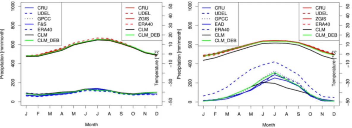
Figure 2.ERA-40, observations and ERA-40 driven COSMO-CLM simulations with (DEB) and without bias correction in the UDRB (left) and the UBRB (right) for the present climate.
– UDEL version 1.02 (Legates and Willmott, 1990): monthly temperature and precipitation data on a global 0.5◦grid for the years 1950–1999
– GPCC full data product version 4 (Schneider et al., 2008): monthly precipitation data on a global 0.5◦grid
for the years 1901–2007
– F&S version 4.1 (Frei and Sch¨ar, 1998): daily precip-itation data on a 1/6◦ grid covering the European Alps
for the years 1971–1999
– EAD v0804 (Xie et al., 2007): daily precipitation data on a 0.5◦ grid covering South East Asia for the years
1980–2002
– ZGIS: a newly developed daily temperature data set on a 0.5◦ grid covering the two basins based on
obser-vational data retrieved from NCDC (http://www.ncdc. noaa.gov/cgi-bin/res40.pl?page=gsod.html), controlled and mapped by the Centre for Geoinformatics, Salzburg (Kienberger et al., 2008).
To quantify the uncertainty of the observational data sets in the basins, a comparison of the climatologic annual cycle in temperature and precipitation was carried out, including ERA-40 re-analysis data.
The downscaling approach developed for and tested on ERA-40 re-analysis data were applied to GCM data. The GCM selection was based on the evaluation of models used in the fourth IPCC assessment report (IPCC, 2007). van Ulden and van Oldenborgh (2006) have investigated 23 GCMs on the quality of simulated global sea level pres-sure patterns. Further, Kripalani et al. (2007) have tested 22 GCMs for their performance in the South Asian region. Amongst these 22 models, they found no best model and a multi model ensemble (MME) mean was proposed as bench-mark. Unfortunately, a multi driving-model ensemble was not feasible in the time frame of BRAHMATWINN and a single GCM had to be selected.
Projections from the selected GCM were then downscaled to a resolution of about 50 km. The dynamical downscaling of four SRES scenarios was followed by a bias correction of the downscaled precipitation and temperature fields tak-ing into account the limited availability of observational data in the UBRB. For other hydro-meteorological fields no bias correction was applied due to lack of quality proofed obser-vational data sets. Further, the impact models used within the BRAHMATWINN framework are assumed to show the highest sensitivity to precipitation and temperature.
4 Results achieved and deliverables provided
4.1 Observation uncertainties
The investigation of different observation data sets in the two basins shows that for precipitation, the uncertainties in the UDRB are relatively small with less than 20 mm month−1
(Fig. 2). Contrary, in the UBRB the data sets differ with a maximum range of 70 mm month−1 in the monsoon months
June to September. However, only small uncertainties ap-pear in the temperature data sets (Fig. 2), both in the UDRB (up to 2.2◦C) and the UBRB (up to 1.2◦C). As the CRU
data set also includes the information on rain day frequency, it was chosen as the observational reference for temperature and precipitation in both basins.
4.2 Downscaling method
To firstly identify an appropriate downscaling method, ERA-40 re-analysis data rather than data from a general GCM sim-ulation have been downscaled from about 1.125◦grid
spac-ing to about 0.5◦. This minimises the influence of large scale
circulation uncertainties on the downscaling results.
40 precipitation. In the UBRB, the COSMO-CLM shows much better results than the ERA-40 precipitation. This has also been expected, since the orography represented by ERA-40 is very coarse and deficiencies in this region are well known (Hagemann et al., 2005).
As the downscaled data was used as input for hydrological modelling (Prasch et al., 2011), a set of hydro-meteorological data (temperature, precipitation, humidity, surface radiation, wind, etc.) was needed. Generating such data sets with statis-tical downscaling methods is highly limited by the sparseness of long term observations which focus mainly on precipita-tion and temperature. Therefore, the dynamical downscaling method is preferable.
4.3 Bias correction
An additional post-processing bias correction has been ap-plied to precipitation and temperature. For precipitation this showed to be problematic in the UBRB, where a high sea-sonality in the COSMO-CLM bias and a large uncertainty in the bias estimation for non-monsoon months have negative impacts on the tested methods (Dobler and Ahrens, 2008). The uncertainties in the bias estimation were found to result from the few rain days in the dry months. To reach the pro-posed minimum number of rain days (about 500) a statistical approach based on local rain day intensity scaling (Schmidli et al., 2006) was developed which corrects the frequency of wet days and the mean wet day precipitation to fit the ob-served values in a specific calibration period. The method uses monthly rainfall amounts and number of rain days, both obtained from the CRU data set. This allows for a longer calibration period (44 yr) than using the EAD data set in the South Asian region. However, to guarantee a robust bias es-timation (and thus correction) the calibration period for the method must still include sufficient rain days. Therefore, the method was applied on a monthly basis to the months June to September in the UBRB only. In the UDRB, the method was applied without monthly splitting as there is almost no seasonality in the COSMO-CLM precipitation bias.
For the 2 m temperature a simple Gaussian bias correction was applied at each grid point. To this end, the simulated
4.4 Downscaling of GCM data
After testing the downscaling approach on ERA-40 forcing data, the method was applied to GCM data from the coupled atmosphere-ocean model ECHAM5/MPIOM (Jungclaus et al., 2006). The ECHAM5/MPIOM for the following reasons was selected to provide the necessary GCM data:
1. It is among the top models simulating a realistic 20th century South Asian monsoon climate (Kripalani et al., 2007).
2. The simulated pressure field has a high skill in the mean spatial correlation and in the mean explained spatial variance for Europe as well as globally (van Ulden and van Oldenborgh, 2006).
3. There is broad experience with the model in downscal-ing applications in Europe
(see, e.g., http://ensembles-eu.metoffice.com and http: //prudence.dmi.dk).
4. It is in good agreement with known large-scale fea-tures of the Asian summer monsoon including the re-establishing of the westerly jets south of the Himalayas and the decay of the anticyclone on the Tibetan Plateau after the monsoon season (data not shown).
5. The COSMO-CLM is able to provide the information necessary for the assessment of regional climate change impacts when driven by the ECHAM5/MPIOM (Dobler and Ahrens, 2010).
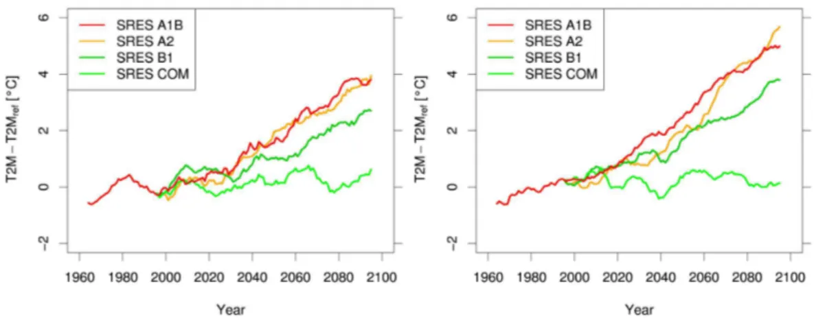
Figure 3.Ten year running means of temperature increase in the UDRB (left) and the UBRB (right) for four SRES scenarios.
Table 1.Description of climate change indicators for precipitation and temperature. The wet/dry day threshold used was 1 mm d−1.
Acronym Description Unit
PFRE Fraction of wet days 1
PREC Total precipitation amount mm
PINT Mean precipitation amount on wet days mm d−1
PQ90 90% quantile of wet days precipitation mm d−1
PX5D Maximum 5-day precipitation amount mm
PCDD Longest period of consecutive dry days d
T2M Mean 2 m temperature ◦C
T2MIN Mean daily minimum 2 m temperature ◦C
T2MAX Mean daily maximum 2 m temperature ◦C
4.5 Regional climate projections
To assess the issue of changing climate in the two basins, seasonal trends of daily precipitation and temperature indi-cators (Table 1) were calculated for the simulation period 1960–2100. For the European regions the seasons are spring (SP, March to May), summer (SU, June to August), autumn (AU, September to November) and winter (WI, December to February). As suggested by Basistha et al. (2009) for the South Asian regions they are summer (SU, March to May), monsoon (MO, June to September), post-monsoon (PM, Oc-tober to November) and winter (WI, December to February). The projections were normalized with respect to the ref-erence period 1971–2000. This is an easy way to remove constant model biases and a comparison to more complex bias correction methods has shown no significant differences in the resulting trends (data not shown). The trends were tested for statistical significance at the 5% level using a lin-ear model.
To give a general summary of the indicator trends is very difficult. The single projections show big regional and sea-sonal differences. But overall, the commitment scenario
shows the smallest trends up to the year 2100, followed by the B1, A1B and finally the A2 scenario. However, up to the year 2080 most A1B trends are higher than those of the A2 scenario (data not shown). This can be explained by the higher emissions of the A1B scenario at the beginning of the 21st century. Thus, the magnitude of the trends is generally in direct relation to the amount of greenhouse gas emissions of the single scenarios.
We will concentrate our evaluations on the results from the scenarios A1B and B1 in the following subsections as they were within the main focus of the BRAHMATWINN project: A1B was considered as the most likely one and B1 as a more optimistic one. However, the projected trends of the A1B and A2 scenario are close to each other. In the commitment sce-nario, constant greenhouse gas concentrations are assumed after the year 2000. Thus, it may be used as a control exper-iment to estimate the impacts of anthropogenic forcings on the climates in the two regions. This is however out of the scope of this study.
4.6 Temperature changes
Figure 3 shows the annual temperature trends for the four SRES scenarios in the two basins. For the A1B scenario, the temperature increase until the year 2100 is projected around 4◦C in the UDRB and 5◦C in the UBRB. For B1 the increase
is around 2◦C in the UDRB and 4◦C in the UBRB.
For A1B the temperature trends are around+3 till+4◦C in
the UDRB and up to more than+6◦C in the UBRB (Fig. 4).
In both basins, the temperature increase in higher elevated areas is larger than in low level areas and the largest trends appear in the region of the Tibetan Plateau. In B1, the trends are about 1◦C smaller than in A1B throughout both basins
(data not shown).
Figure 4.Linear trends of the annual mean temperature (◦C/cent.) in the UDRB (left) and the UBRB (right) during the time period 1960– 2100 following the A1B scenario. Coloured areas show significant trends (at the 5% level). The grey dotted lines denote isohypses in m a.s.l. Also shown are the Lech (white) and the Salzach (blue) river basin on the left and the Assam region (blue), the Lhasa (green) and the Wang-Chu (brown) river basin on the right.
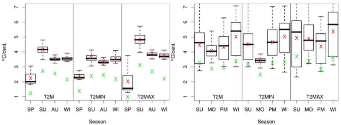
Figure 5.Spatial variability of seasonal trends in T2M, T2MIN and T2MAX in the UDRB (left) and the UBRB (right) for the A1B scenario. Red and green crosses show statistically significant spatial mean trends for the A1B and the B1 scenario, respectively.
green cross for the B1 scenario. As can be seen, both scenar-ios show significant positive trends for all seasons in temper-ature, as well as daily minimum and maximum temperature in both basins. The increase of the maximum daily temper-ature is generally highest, followed by the increase of mean temperature and the increase of the daily minimum tempera-ture suggesting an increase in temperatempera-ture variability. How-ever, there are also exceptions to this, for instance during the post-monsoon season in the UBRB and spring in the UDRB.
4.7 Precipitation changes
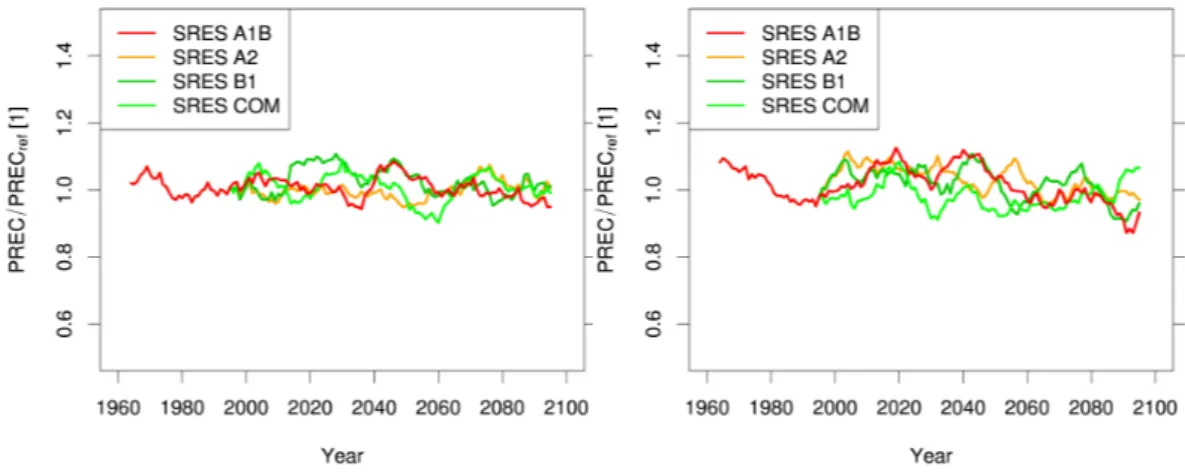
The projected precipitation trends are less unanimous than the temperature trends. No significant trends were found in the two basins for the annual precipitation amounts (Fig. 6). This is however a result of trends compensating each other in the different seasons and areas.
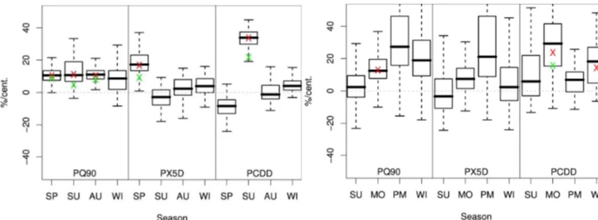
Figures 7 and 8 show the trends of precipitation-based indicators in the UDRB and UBRB. In A1B, the
sum-mer precipitation amount in the UDRB is decreasing with about 20%/century and the monsoon precipitation amount in the UBRB with about 10%/century (Fig. 7). Simultane-ously, there is a decrease in the number of precipitation days (PFRE), an increase in the rain-day intensity (PINT) as well as an increase in the length of consecutive dry days (PCDD) in both basins (Fig. 8).
In the UDRB there is further an increase of PREC (Fig. 7) and of PX5D (Fig. 8) in spring. As can be seen, there are less significant precipitation trends in the UBRB than in the UDRB which is due to a larger inter-annual variability (data not shown). In both basins, the PQ90 trends agree to a large extend with the trends in PINT for all seasons.
Figure 6.Ten year running means of precipitation change in the UDRB (left) and the UBRB (right) for four SRES scenarios.
Figure 7.As for Figure 5, but for PREC, PFRE and PINT.
these trends are about 50% smaller but the spatial distribu-tion is similar (data not shown).
Figure 9 and the high temperature increases shown above indicate that the Tibetan Plateau is a region highly sensitive to future climate changes. For Assam, the positive trend in PCDD implies longer monsoon breaks, which in the current climate show a typical length of 15 days.
5 Contributions to sustainable IWRM
The presented GCM downscaling approach provided the ba-sis for the integrated water resources management system comprising the DANUBIA hydrological model, the river basin information system (RBIS) and the network analysis and creative modelling decision support system NetSyMoD which is building a sustainable development based on stake-holder negotiations within the framework of the project.
The results shown in this paper provide sound evidence about likely climate change dynamics which will impact the hydrological process dynamics and runoffgeneration at present active within both twinning basins. They provide a scenario based framework setup within which adaptive
man-agement options for sustainable IWRM can be developed and evaluated.
The results discussed focus on the most pronounced trends in the UDRB and the UBRB during the years 1960–2100. A complete set of time series for all scenarios, seasons, ar-eas of interest (see Fig. 4) and the indicators PREC, PX5D, PCDD, T2M, T2MIN and T2MAX (Table 1) for the years 1960–2100 are available through the RBIS of the BRAH-MATWINN project.
6 Conclusions and recommendations
Using regional climate projections from the COSMO-CLM allows analysing the impact of the climate change signal on the regional water balance in the UDRB and the UBRB. To generate several likely scenarios for the time period 1960–2100, the COSMO-CLM was driven by the GCM ECHAM5/MPIOM with four different SRES forcing. The model output was for instance used as input to the hydrolog-ical model DANUBIA.
Figure 8.As for Figure 5, but for PQ90, PX5D and PCDD.
Figure 9.Linear trends (%/cent.) of PX5D (left) and PCDD (right) in the UBRB in the monsoon season from 1960 to 2100 following the A1B scenario. White areas show non-significant trends (at the 5% level). The grey dotted lines denote isohypses in m a.s.l. Coloured lines show the Assam region (blue), the Lhasa (green) and the Wang-Chu (brown) river basin.
the Tibetan Plateau. Thus, parameters directly dependent on temperature, like potential evapotranspiration, are also as-sumed to show clear trends. This will have a severe impact on the hydrology of the river basins.
Precipitation trends are less clear. Annual precipitation is projected not to change significantly, but seasonal amounts are. Different climate change indicators, like the length of the longest dry periods, indicate more frequent and prolonged droughts. However, there is no simultaneous tendency to less flooding events. The projected increasing amount of (1-day and 5-day) spring precipitation in the UDRB in combination with increased spring snow melt due to higher temperatures in the Alps might even yield more intense and frequent flood-ing events.
An increase in the number of consecutive dry days and in the maximum 5-day precipitation amount in the region of the Tibetan Plateau for the monsoon season, as well as large temperature trends indicate a highly sensitive region to future climate changes. For Assam, the positive trend in the num-ber of consecutive dry days in the monsoon season indicates longer monsoon breaks.
Acknowledgements. This work was funded by the EC project BRAHMATWINN, contract 036592 (GOCE). The authors also acknowledge support in using the CLM by the COSMO-CLM community and funding from the Hessian initiative for the development of scientific and economic excellence (LOEWE) through the Biodiversity and Climate Research Centre (BiK-F), Frankfurt/Main. Computational time was provided by the German Climate Computing Centre (DKRZ) and the Swiss National Supercomputing Centre (CSCS).
The interdisciplinary BRAHMATWINN EC-project carried out between 2006–2009 by European and Asian research teams in the UDRB and in the UBRB enhanced capacities and supported the implementation of sustainable Integrated Land and Water Resources Management (ILWRM).
References
Ahrens, B.: Evaluation of precipitation forecasting with the lim-ited area model ALADIN in an alpine watershed, Meteor. Z., 12, 245–255, 2003.
Basistha, A., Arya, D. S., and Goel, N. K.: Analysis of historical changes in rainfall in the Indian Himalayas, Int. J. Climatol., 29, 555–572, doi:10.1002/joc.1706, 2009.
Bates, B., Kundzewicz, Z., Wu, S., and Palutikof, J. (Eds.): Cli-mate change and water, IPCC Technical Paper, IPCC Secretariat, Geneva, Switzerland, 2008.
Beck, A., Ahrens, B., and Stadlbacher, K.: Impact of nesting strate-gies in dynamical downscaling of reanalysis data, Geophys. Res. Lett., 31, L19101, doi:10.1029/2004GL020115, 2004.
Dobler, A. and Ahrens, B.: Precipitation by a regional climate model and bias correction in Europe and South Asia, Meteor. Z., 17, 499–509, 2008.
Dobler, A. and Ahrens, B.: Analysis of the Indian summer monsoon system in the regional climate model COSMO-CLM, J. Geophys. Res., 115, D16101, doi:10.1029/2009JD013497, 2010.
Doms, G. and Sch¨attler, U.: The nonhydrostatic limited-area model LM of DWD. Part 1: Scientific documentation, available at: http:
//www.cosmo-model.org, 1999.
Frei, C. and Sch¨ar, C.: A precipitation climatology of the Alps from high-resolution rain-gauge observations, Int. J. Climatol, 18, 873–900, 1998.
Frei, C., Christensen, J., Deque, M., Jacob, D., Jones, R., and Vi-dale, P.: Daily precipitation statistics in regional climate models: Evaluation and intercomparison for the European Alps, J. Geo-phys. Res., 108, 4124, doi:10.1029/2002JD002287, 2003. Giannini, V. and Giupponi, C.: Integration by identification of
indi-cators, Adv. Sci. Res., this special volume, 2011a.
Giannini, V., Giupponi, C., Hutton, C., Allan, A. A., Kienberger, S., Fl¨ugel, W.-A., and Ceccato, L.: Development of IPCC based “what-if?” IWRM scenarios, Adv. Sci. Res., this special volume, 2011b.
Hagemann, S., Arpe, K., and Bengtsson, L.: Validation of the hy-drological cycle in ERA-40, Tech. Rep., ECMWF, 2005. IPCC: Climate Change 2007: Synthesis Report. Contribution of
Working Groups I, II and III to the Fourth Assessment Report
of the Intergovernmental Panel on Climate Change [Core Writ-ing Team, Pachauri, R. K. and ReisWrit-inger, A. (Eds.)], IPCC, 2007. Jones, C., Gregory, J., Thorpe, R., Cox, P., Murphy, J., Sexton, D., and Valdes, H.: Systematic optimization and climate simulation of FAMOUS, a fast version of HADCM3, Hadley Centre Tech-nical Note, 60, 33, 2004.
Jungclaus, J. H., Keenlyside, N., Botzet, M., Haak, H., Luo, J. J., Latif, M., Marotzke, J., Mikolajewicz, U., and Roeckner, E.: Ocean circulation and tropical variability in the coupled model ECHAM5/MPI-OM, J. Climate, 19, 3952–3972, 2006.
Kienberger, S., Tiede, D., Ungersb¨ock, M., Klug, H., and Ahrens, B.: Interpolation of daily temperature values for european and asian test-areas, in: Geospatial Crossroads @ GI Forum ’08, edited by: Car, A., Griesebner, G., and Strobl, J., Wichmann Verlag, 164–169, 2008.
Kothe, S., Dobler, A., Beck, A., and Ahrens, B.: The
ra-diation budget in a regional climate model, Clim. Dynam., doi:10.1007/s00382-009-0733-2, 2010.
Kripalani, R., Oh, J. H., Kulkarni, A., Sabade, S. S., and Chaudhari, H. S.: South Asian summer monsoon precipitation variability: Coupled climate model simulations and projections under IPCC AR4, Theor. Appl. Clim., 90, 133–159, doi:10.1007/ s00704-006-0282-0, 2007.
Kumar, K. R., Sahai, A. K., Kumar, K. K., Patwardhan, S. K., Mishra, P. K., Revadekar, J. V., Kamala, K., and Pant, G. B.: High-resolution climate change scenarios for India for the 21st century, Curr. Sci., 90, 334–345, 2006.
Lang, S., K¨a¨ab, A., Pechst¨adt, J., Fl¨ugel, W.-A., Zeil, P., Lanz, E., Kahuda, D., Frauenfelder, R., Casey, K., F¨ureder, P., Sossna, I., Wager, I., Janauer, G., Exler, N., Boukalova, Z., Tapa, R., Lui, J., and Sharma, N.: Assessing components of the natural environ-ment of the Upper Danube and Upper Brahmaputra river basins, Adv. Sci. Res., this special volume, 2011.
Legates, D. R. and Willmott, C. J.: Mean seasonal and spatial vari-ability in gauge-corrected, global precipitation, Int. J. Climatol., 10, 111–127, 1990.
Mitchell, T. D. and Jones, P. D.: An improved method of construct-ing a database of monthly climate observations and associated high-resolution grids, Int. J. Climatol., 25, 693–712, 2005. Murphy, J.: An evaluation of statistical and dynamical techniques
for downscaling local climate, J. Climate, 12, 2256–2284, 1999. Nakicenovic, N. and Swart, R.: Special Report on Emissions Sce-narios, Cambridge University Press, Cambridge, UK, p. 612, 2000.
Prasch, M., Marke, T., Strasser, U., and Mauser, W.: Large scale in-tegrated hydrological modelling of the impact of climate change on the water balance with DANUBIA, Adv. Sci. Res., this special volume, 2011.
Salath´e, E. P.: Comparison of various precipitation downscaling methods for the simulation of streamflow in a rainshadow river basin, Int. J. Climatol., 23, 887–901, doi:10.1002/joc.922, 2003.
Schmidli, J., Frei, C., and Vidale, P. L.: Downscaling from
GCM precipitation: A benchmark for dynamical and statis-tical downscaling methods, Int. J. Climatol., 26, 679–689, doi:10.1002/joc.1287, 2006.