Restoration via a Kinetics-Induced Bilateral Filter
Zhaoying Bian, Jing Huang, Jianhua Ma*, Lijun Lu, Shanzhou Niu, Dong Zeng, Qianjin Feng, Wufan Chen
School of Biomedical Engineering, Southern Medical University, Guangzhou, China
Abstract
Dynamic positron emission tomography (PET) imaging is a powerful tool that provides useful quantitative information on physiological and biochemical processes. However, low signal-to-noise ratio in short dynamic frames makes accurate kinetic parameter estimation from noisy voxel-wise time activity curves (TAC) a challenging task. To address this problem, several spatial filters have been investigated to reduce the noise of each frame with noticeable gains. These filters include the Gaussian filter, bilateral filter, and wavelet-based filter. These filters usually consider only the local properties of each frame without exploring potential kinetic information from entire frames. Thus, in this work, to improve PET parametric imaging accuracy, we present a kinetics-induced bilateral filter (KIBF) to reduce the noise of dynamic image frames by incorporating the similarity between the voxel-wise TACs using the framework of bilateral filter. The aim of the proposed KIBF algorithm is to reduce the noise in homogeneous areas while preserving the distinct kinetics of regions of interest. Experimental results on digital brain phantom andin vivorat study with typical18F-FDG kinetics have shown that the present KIBF algorithm can achieve notable gains over other existing algorithms in terms of quantitative accuracy measures and visual inspection.
Citation:Bian Z, Huang J, Ma J, Lu L, Niu S, et al. (2014) Dynamic Positron Emission Tomography Image Restoration via a Kinetics-Induced Bilateral Filter. PLoS ONE 9(2): e89282. doi:10.1371/journal.pone.0089282
Editor:Marc Dhenain, CNRS, France
ReceivedAugust 21, 2013;AcceptedJanuary 19, 2014;PublishedFebruary 27, 2014
Copyright:ß2014 Bian et al. This is an open-access article distributed under the terms of the Creative Commons Attribution License, which permits unrestricted use, distribution, and reproduction in any medium, provided the original author and source are credited.
Funding:This work was partially supported by the National Natural Science Foundation of China (http://www.nsfc.gov.cn/) under grants No. 81000613 and No. 81101046; the National Key Technology Research and Development Program of the Ministry of Science and Technology of China (http://kjzc.jhgl.org/) under grant No. 2011BAI12B03; the Science and Technology Program of Guangdong Province of China (http://www.gdstc.gov.cn/) under grant No. 2011A030300005; National Key Scientific Instrument and Equipment Development Project of China (http://www.nmp.gov.cn/) under grant No. 2011YQ03011404; and the 973 Program of China (http://www.973.gov.cn/) under grant No. 2010CB732504. The funders had no role in study design, data collection and analysis, decision to publish, or preparation of the manuscript.
Competing Interests:The authors have declared that no competing interests exist. * E-mail: [email protected] (JM)
Introduction
Dynamic positron emission tomography (PET) is a powerful tool that provides useful quantitative information on physiological and biochemical processes [1]. Associative parametric imaging can be achieved by fitting the time activity curves (TACs) at each voxel with a linear or nonlinear kinetic model [2]. However, low signal-to-noise ratio (SNR) in short dynamic frames causes the related noise to be inevitably transferred to the voxel-wise kinetic parameter estimation from the TAC measurements. Thus, PET parametric imaging is essentially an ill-posed problem.
As regards PET parametric imaging, the related reconstructions can be realized by using direct and indirect methods [3–5]. Direct reconstruction methods enable accurate compensation of noise propagation from the projection data to the kinetic fitting process by combining kinetic modeling and dynamic image reconstruction into a unitary formula [6–9]. Direct reconstruction methods usually require knowledge of the input function, that is, the TAC of tracer concentration in arterial blood. The related data acquisition is known to be invasive and labor intensive, which limits its application in clinical practice. As regards indirect reconstruction methods, dynamic image reconstruction and kinetic analysis are conducted separately. Meanwhile, the image-derived input function method [9–13] or reference region method [14,15] can be employed as an alternative to painful blood sample measurement. To achieve high-quality dynamic PET images, two strategies are commonly used, namely, maximum a posteriori
images [38]. In addition, by considering the dynamic PET TAC in each voxel as a vector, Tauber et al.designed a spatio-temporal anisotropic diffusion image filter with noticeable gains over the existing methods [20].
In this work, to improve PET parametric imaging accuracy, we present a kinetics-induced bilateral filter (KIBF) to reduce the noise of dynamic image frames by incorporating the similarity between the voxel-wise TACs using the framework of BF [39]. The aim of the present KIBF algorithm is to reduce the noise in homogeneous areas while preserving the distinct kinetics of regions of interest (ROIs). To validate and evaluate the performance of the proposed KIBF algorithm, experiments were conducted through computer simulations and a preclinical rat study with a focus on quantitative accuracy measures and visual inspection.
Materials and Methods
Ethics Statement
The rat study was conducted in strict accordance with the recommendations in the Guide for the Care and Use of Laboratory Animals of the National Institutes of Health. The protocol was approved by the Institutional Animal Care and Use Committee of Case Western Reserve University (Permit Number: 2008-0072). All surgery was performed under 2% isoflurane anesthesia, and all efforts were exerted to minimize suffering.
Brief Review of the BF
The BF was originally proposed by Tomasi and Manduchi for 2D image processing [39]. The discrete version of their BF algorithm can be expressed as follows: LetBbe a discrete grid of voxels and x~fx(i)Di[Bg be a noisy image. Given a neighbor
windowNi5Bcentered at voxeli, the restored intensityBF(x)(i)
at voxel i is the weighted average of all intensities of the neighboring voxelsfjDj[Nigand can be written as
BF(x)(i)~X
j[Niw(i,j)x(j) ð1Þ
wherex(j)denotes the image intensity at voxelj, andw(i,j)is the weight and consists of a product of two separate filters acting in the spatial and intensity domains. The popular weightw(i,j)is often defined as Gaussian shape:
w(i,j)~ 1
S(i)exp { (i{j)2
2s2
s
( )
:exp {(x(i){x(j)) 2
2s2
x
( )
ð2Þ
where
S(i)~Pj[N
iexp {(i{j)
2=(2s2
s)
:
exp {(x(i){x(j))2=(2s2
x)
is a normalizing factor to ensure that the weightw(i,j)satisfies the conditions of0ƒw(i,j)ƒ1andP
j[Niw(i,j)~1. Two parameters ss and sx control the geometric proximity and the intensity
similarity, respectively.
Description of the KIBF
Our proposed KIBF adapts the concept of the BF algorithm to make use of both the spatial information and the voxel-wise kinetic information within the entire dynamic PET data. The KIBF algorithm contains two major steps: (a) optimal weight construc-tion using kinetics informaconstruc-tion; and (b) weighted average using the constructed weights.
Optimal Weight Construction. In dynamic PET studies, voxels in physiologically similar regions have similar tissue TAC kinetics. Thus, the TAC tendency can provide the tissue-specific biochemical information for dynamic PET image filtering. Under the framework of the BF algorithm, the weights can be optimally constructed by exploring the voxel-wise kinetic information. In this work, by incorporating the similarity between the voxel-wise TACs, the optimal weights are constructed as follows:
~ w w(i,j)~ 1
~ S
S(i)exp { (i{j)2
2s2
s
( )
:exp {kZ(i){Z(j)k 2
W
2s2
z
( )
ð3Þ
where
S(i)~Pj[N
i exp {(i{j)
2=(2s2
s)
:
expn{kZ(i){Z(j)k2W=
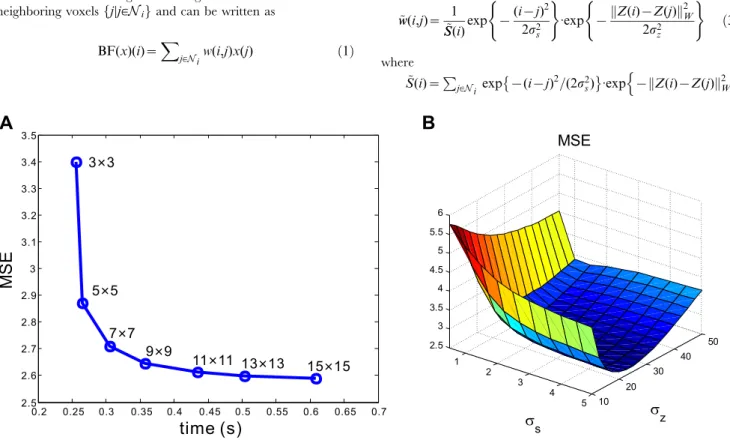
Figure 1. Two MSE plots or parameter selections of the neighbor window (A) and the controlling parameters (B) of KIBF algorithm.
doi:10.1371/journal.pone.0089282.g001
(2s2
z)gis the normalizing factor. The TAC at voxelkis denoted as Z(k)~fx(k,t),t~1,2, ,Tg, where x(k,t) denotes the activity value of voxel k(k~i,j) at framet, and T is the total sampling time frames. The similarity measure between two TACs is calculated by the distance measure k k: 2W, which is defined as
Y
k k2W~ PT
t~1W(t)Y2(t), where W is the vector of weighting factors. An empirical choice of W is W~fDtt,t~1,2, ,Tg,
wherein Dtt denotes the time duration of the sampling framet.
Two factorsssandszcontrol the spatial voxel neighborhood and
the TAC similarity, respectively.
Weighted Average. Based on the constructed weightsww~(i,j), a voxel-wise weighted average operation similar to Equation (1) can be performed on each frame. The present KIBF algorithm can be described as follows:
KIBF(x)(i,t)~X
j[Niww~(i,j)x(j,t): ð4Þ
Given that the average weights at voxel iare the same for each frame, the present KIBF algorithm can also be directly performed on the noisy TACs as follows:
KIBF(Z)(i)~X
j[Niww~(i,j)Z(j): ð5Þ
The weighted average of Equation (5) illustrates that the present KIBF algorithm takes advantage of both the spatial and temporal consistencies of the dynamic PET data. As a result, the noise in each individual frame can be remarkably suppressed by the introduction of voxel-wise kinetic information within the entire dynamic frames.
Parameter Selection for the KIBF Algorithm
For the present KIBF algorithm, three parameters will be determined, namely, the size of the neighbor windowNiand the
controlling parameters ss and sz. In this study, the minimum
mean squared error (MSE) measure and visual inspection of clinical experts were used for parameter selection. The MSE between the original and de-noised dynamic images is defined as MSE(F(Xnoise,h) )~ F(Xnoise,h){Xphantom
2
=M, where
Xnoise is the noisy dynamic image, Xphantom is the original
phantom dynamic image,M is the total number of voxels, F (:)
denotes the filtering processing andh is the filter parameter or parameter set (h~fss,szgfor the present KIBF algorithm) to be
determined. Visual inspection was conducted by clinical experts to score from 0 (worst) to 10 (best) for two aspects (namely, noise reduction and edge-preservation) separately for each displayed image set. The higher score indicates the better parameter setting. In the computer simulations, as the ground truth is known, the parameters were all selected by minimizing the MSE with optimized parameter settings. In the preclinical rat study, two clinical experts were asked to score the resultant images in terms of visual inspection on noise reduction and edge-preservation. The resultant images with different parameter settings of the same subject were randomized in order and displayed on the computer screen. The display did not have any indication of which parameter setting was used for the displayed images. Therefore the procedure was completely blind.
Selection of Neighbor Window. To exploit the neighbor-hood and similarity information fully for the KIBF algorithm, the neighbor window sizeNi should be sufficiently large. However,
the associated computational load will be increased. In this study, extensive experiments with minimum MSE measure and visual inspection from two clinical experts have shown that a 7|7 neighbor window was adequate for effective noise reduction while
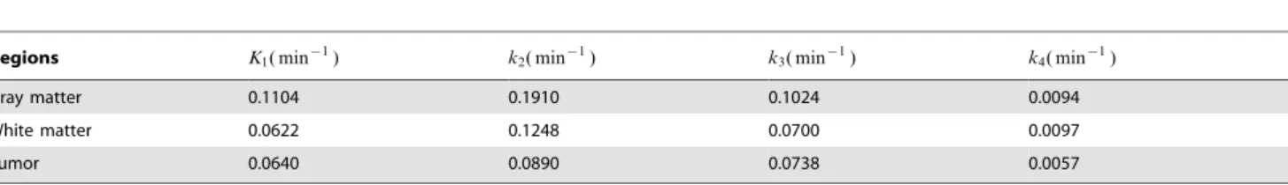
Table 1.Kinetic parameters used in the18F-FDG PET simulation.
Regions K1( min{1) k2( min{1) k3( min{1) k4( min{1)
Gray matter 0.1104 0.1910 0.1024 0.0094
White matter 0.0622 0.1248 0.0700 0.0097
Tumor 0.0640 0.0890 0.0738 0.0057
doi:10.1371/journal.pone.0089282.t001
Figure 2. The18F-FDG PET simulation settings.(A) A brain phantom composed of gray matter, white matter and a small tumor; (B) the blood input function and regional time activity curves.
retaining computational efficiency. The MSE plot for the selection of the neighbor window size is shown in Figure 1A.
Selection of Controlling Parameters. Similar to the BF algorithm, the performance of the KIBF algorithm depends on the selection of two controlling parameters ss and sz. In the
implementation, if ss and sz are extremely large, the KIBF
filtered images will suffer from smeared edges, whereas the values are extremely small, the desired results cannot achieve noise suppression. Thus, a tradeoff between noise suppression and edge preservation should be achieved by optimizing the two controlling parametersssandsz with some reliable image quality measures.
In this study, the MSE estimation was used for the computer
simulation experiments, and visual inspection by two clinical experts was used for the preclinical rat experiments. Extensive experiments have shown that ss~4 voxel and sz~20 were appropriate for the simulation studies as shown in Figure 1B, and
ss~4 voxel andsz~0:25were adequate for the preclinical rat
studies.
Data Acquisitions
Computer Simulations. A digital brain phantom [7,8], as shown in Figure 2A, which consists of gray matter, white matter, and a small tumor within the white matter, was used for the computer simulations. In the simulations, we selected a two-tissue
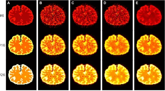
Figure 4. The ground truth and the activity images reconstructed by different algorithms at frames#6,#16, and#26.(A) are the ground truth; (B) are the results from the direct FBP reconstruction; (C) are the results from the FBP images filtered by the GF algorithm (sg~0:5
voxel); (D) are the results from the FBP images filtered by the BF algorithm (ss~4voxel,b~0:5); and (E) are the results from the FBP images filtered
by the present KIBF algorithm (ss~4voxel,sz~20). All images are with a same display window. doi:10.1371/journal.pone.0089282.g004
Figure 3. MSE plots for parameter selections of the standard deviation for GF algorithm (A) and the controlling parameters of BF algorithm (B).
compartment and 18F-FDG based tracer kinetic model for glucose metabolism imaging of brain. Based on Feng’s model described in [40], the TAC of each region was generated according to the two-tissue compartment model and an analytical blood input function as shown in Figure 2B. The calculation of the kinetic model and the fitting procedure were performed using the COMKAT package (http://comkat.case.edu) [41]. Given the clinical application of the present algorithm, the kinetic param-eters K1,k2,k3,k4 estimated from a set of 70 studies on brain tumor patients described in [42] were used in our simulation and they are listed in Table 1. In this study, the influx rate
Ki~K1k3=(k2zk3), which is related to the glucose metabolic rate by a scaling factor, was analyzed. In addition, the fractional volume of blood in the tissue was set to zero for three target regions. The scanning schedule of dynamic PET data consists of 30 time frames: 4|20 s, 4|40 s, 4|60 s, 4|180 s, and
14|300 s. The TACs were integrated for each frame and
forward projected to generate dynamic sinograms and then Poisson noise was added, which resulted in an expected total number of events over 90 min that is equal to 50 million. A filtered back-projection (FBP) method with a ramp filter was used for the dynamic PET reconstruction.
Preclinical Dynamic PET Data. The preclinical dynamic PET data were acquired from a female 236 g Sprague-Dawley rat [43]. The rat was injected intravenously with 30.7 MBq of18 F-FDG and scanned with a micro-PET R4 system (Siemens Medical Solutions USA, Inc.). The PET scanning schedule was 12|5 s, 12|30 s, 5|60 s, and 15|300 s. Corrections for radioactive decay, attenuation, scatter, and dead time were performed before image reconstruction. The dynamic PET images were recon-structed using an image matrix of 128|128|63 with voxel sizes of 0.4922|0.4922|1.220mm3 for each frame. An ordered subset expectation maximization (OSEM) algorithm [44] with 16 subsets and 4 iterations was used for all reconstructions. In addition, blood sampling was performed to provide a gold-standard reference, and the input function from the samples was linearly interpolated to construct a final input function. Similar to the computer simulations, the influx rateKiparametric image was
calculated based on the final input function.
Comparison Algorithms
To validate and evaluate the performance of the present KIBF algorithm, the Gaussian filter (GF) and the BF algorithms were adopted for comparison.
GF. The following GF algorithm was implemented for each image frame separately:
GF(x)(i,t)~X
j[Vi
exp {(i{j)2=(2s2
g)
P
k[Vi exp {(i{k)
2=(2s2
g)
x(j,t) ð6Þ
whereViis the neighbor window, andsgis the standard deviation
of the Gaussian function that determines the width of the Gaussian kernel. For each image frame, the parameter sg was chosen
empirically to yield a minimum MSE as shown in Figure 3A and good visual inspection by two clinical experts.
BF. The BF algorithm, as described in Equations (1) and (2), was also applied to each frame separately. Considering the variation of the activity value among different image frames, we proposed a frame-dependent scale parameter form, that is,
sx,t~bst, to control the image intensity similarity at frame t,
wherebis a scaling factor, andstis the estimated noise standard
deviation of framet. The calculation ofstis the same as that used
in our previous work [18]. In the implementation, a 7|7 neighbor window was used for the BF algorithm. The parametersssandb
were determined by extensive experiments using minimum MSE Figure 5. Three TAC plots from different algorithms for the corresponding voxels located in the gray matter (A), white matter (B) and small tumor regions (C), respectively.
estimation, as shown in Figure 3B, and visual inspection by two clinical experts.
Results
Phantom Study
Comparison of Dynamic PET Activity Images. Figure 4
shows the ground truth and the activity images reconstructed by different algorithms at frames #6, #16, and #26. The first column represents the ground truth, the second column shows the results from the direct FBP reconstruction, the third column shows the results from the FBP image filtered by the GF algorithm (sg~0:5voxel), the fourth column shows the results from the FBP
image filtered by the BF algorithm (ss~4voxel,b~0:5); and the
fifth column presents the results from the FBP image filtered by the present KIBF algorithm (ss~4 voxel, sz~20). The results
demonstrate that the KIBF algorithm can yield significant noise reduction without concealing subtle information compared with other algorithms. To illustrate the effect of temporal information on the smoothing of dynamic frames, we extracted the TACs of three voxels located within the gray matter, the white matter, and the small tumor regions, respectively. Figure 5 shows the TAC plots from different algorithms for the corresponding voxels. We can see that the TACs resulting from the present KIBF algorithm are closer to the ground truth and smoother compared with those of the other three algorithms. Figure 6 shows the box plots of the mean activities with standard deviations in the gray matter, white matter and small tumor regions from different algorithms at
frames #6, #16, and #26. We find that the present KIBF algorithm achieves less bias compared with the ground truth as well as less standard deviation than the other algorithms.
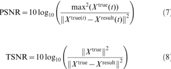
Furthermore, the merits of peak signal-to-noise ratio (PSNR) for each individual frame and the total signal-to-noise ratio (TSNR) for entire dynamic frames were used to measure the bias between the ground truth and estimated values with different algorithms, which is defined as
PSNR~10 log10
max2(Xtrue(t))
Xtrue(t){Xresult(t)
k k2
!
ð7Þ
TSNR~10 log10
Xtrue
k k2
Xtrue{Xresult
k k2
!
ð8Þ
whereXtruedenotes the original phantom image,Xresult denotes the filtered result,Xtrue(t)andXresult(t)denote the corresponding image at framet, and max2(Xtrue(t)) represents the maximum activity value of the original phantom image at framet. Figure 7 plots the PSNRs at each frame of the activity images reconstructed by the FBP, GF, BF and KIBF algorithms. The PSNR curves illustrate that KIBF has a noticeable gain over the GF and BF algorithms in terms of PSNR measurement, particularly in the early frames. Table 2 lists the TSNRs of the activity images reconstructed by different algorithms. The KIBF algorithm Figure 6. Box plots of the mean activities with standard deviations in the gray matter, white matter and small tumor regions from different algorithms at (A) the frame#6; (B) the frame#16; and (C) the frame#26.
doi:10.1371/journal.pone.0089282.g006
Figure 7. PSNRs at each frame of the activity images reconstructed by different algorithms.
achieves more noticeable gains over other two algorithms in terms of TSNR measurement.
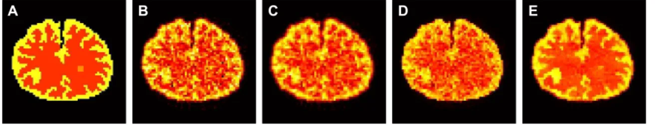
Comparison of PET Parametric Images. Figure 8 shows
the ground truth and the estimatedKiparametric images from the
activity images reconstructed by different algorithms: (A) is the ground truth; (B) is the result from the direct FBP reconstruction; (C) is the result from the FBP image filtered by the GF algorithm (sg~0:5voxel); (D) is the result from the FBP image filtered by the
BF algorithm (ss~4voxel,b~0:5); and (E) is the result from the
FBP image filtered by the present KIBF algorithm (ss~4voxel, sz~20). The KIBF algorithm can achieve better performance
than other algorithms in terms of both noise reduction and the detailedKiparametric information estimation. Figure 9 represents
a description of the mean value ofKiand the standard deviations
in the gray matter, white matter, and small tumor regions by different algorithms. We find that the KIBF algorithm achieves less bias compared with the ground truth as well as less standard deviation than the other algorithms.
To evaluate the performance of the KIBF algorithm quantita-tively, the regional normalized standard deviation (NSD) versus bias tradeoff curves were studied. Borrowing the definitions in [31], NSD and Bias are written as:
NSDroi~
ffiffiffiffiffiffiffiffiffiffiffiffiffiffiffiffiffiffiffiffiffiffiffiffiffiffiffiffiffiffiffiffiffiffiffiffiffiffiffiffiffiffiffiffiffiffiffiffiffiffiffiffiffiffi
1
Mroi{1
P
j[roiðKi(j){KKroiÞ2
q
K Kroi
|100% ð9Þ
Biasroi~
K
Kroi{Kroitrue
Ktrue roi
|100% ð10Þ
where Ki(j) denotes the estimatedKi parametric value at voxel j(j~1,2, ,Mroi) in the region of interest (ROI),
K
Kroi~Pj[roiKi(j)=Mroi denotes the mean of the estimated Ki
parametric value in the ROI, andMroirepresents the number of voxels in the ROI. For the regional bias (Biasroi), Kroitrue is the
known uniform parametric value in the ROI. To quantify NSD versus Bias in the whole brain region for an overall assessment of quantitative performance,NSDroiandBiasroivalues for the ROIs (gray matter, white matter, and small tumor) were averaged, and weighted based on the size (number of voxelsMroi)in each ROI. Figure 10 shows the NSD versus Bias tradeoff curves of the influx rateKiestimated by the GF, BF, and KIBF algorithms for
different ROIs in the brain phantom. The parametric images generated from the filtered dynamic activity images with the KIBF algorithm outperform those generated by the other two algorithms based on the NSD versus Bias tradeoff analysis.
Preclinical Rat Study
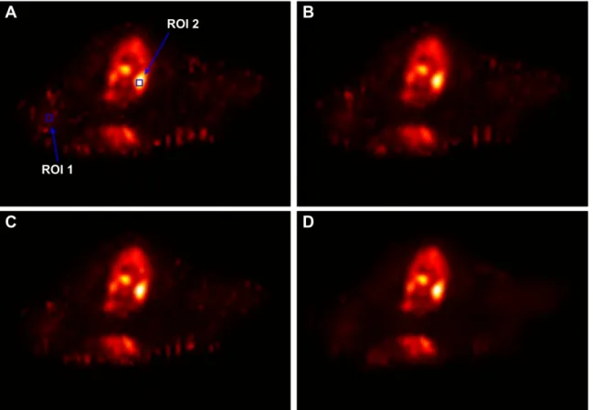
Figure 11 shows the transaxial slices ofKi parametric images
estimated from: (A) the direct OSEM reconstruction, (B) the OSEM images filtered by the GF algorithm (sg~0:5voxel), (C)
the OSEM images filtered by the BF algorithm (ss~4 voxel, b~2), and (D) the OSEM images filtered by the present KIBF algorithm (ss~4 voxel, sz~0:25). The KIBF algorithm can achieve better performance than other algorithms in terms of both noise reduction and detailedKi parametric information
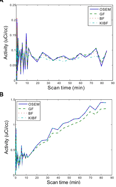
estima-tion. Moreover, in the preclinical rat study, we extracted the TACs of two voxels located within a low glucose metabolic region (ROI 1) and a high glucose metabolic region (ROI 2), respectively. The ROIs were indicated by the squares in Figure 11(A). Figure 12 shows the TAC plots from different algorithms for the corre-sponding voxels. In the low glucose metabolic region, the noise is suppressed strongly by the present KIBF algorithm and the corresponding TAC seems smoother than those resulted from the other algorithms; while in the high metabolic region, the noise is suppressed slightly by the present KIBF algorithm. The results could illustrate that the different smooth strength is dependent on the noise level, and the high glucose metabolic region has a less noise level than the low glucose metabolic region.
Discussion
To improve PET parametric imaging accuracy, the BF algorithm has been investigated with significant gains over the GF algorithm in terms of noise reduction and resolution preservation [19]. However, as a spatial filter, the BF algorithm merely reduces the noise of individual frames without considering the kinetic information contained in all dynamic images. In this study, we developed the KIBF algorithm to reduce the noise of dynamic images by incorporating the kinetic information using the framework of the BF algorithm. The KIBF algorithm can be
Figure 8. The ground truth and the estimatedKiparametric images from the activity images reconstructed by different algorithms.
(A) is the ground truth; (B) is the result from the direct FBP reconstruction; (C) is the result from the FBP image filtered by the GF algorithm (sg~0:5
voxel); (D) is the result from the FBP image filtered by the BF algorithm (ss~4voxel,b~0:5); and (E) is the result from the FBP image filtered by the
present KIBF algorithm (ss~4voxel,sz~20). All images are with a same display window.
doi:10.1371/journal.pone.0089282.g008
Table 2.The TSNRs of the activity images reconstructed by different algorithms.
Methods FBP GF BF KIBF
TSNRs (dB) 12.92 13.24 13.93 16.29
regarded as a combination of the spatial domain filter and the temporal TAC filter, as expressed in Equation (3). As a spatio-temporal filter, the KIBF algorithm can reduce the noise in homogeneous areas while preserving the distinct kinetics of ROIs.
Moreover, considering the nature of the KIBF calculated from the associative TACs, the algorithm does not require any prior kinetic models typically used in existing approaches [6,29,30]. Thus, the KIBF algorithm can be a potential tool to realize accurate
Figure 10. The NSD versus Bias tradeoff curves of the influx rateKiestimated by the GF, BF and KIBF algorithms for different ROIs in the brain phantom.
doi:10.1371/journal.pone.0089282.g010
Figure 9. Box plots of the mean value ofKiwith standard deviations in the gray matter, white matter and small tumor regions from different algorithms.
dynamic PET imaging. The preliminary results have shown that the KIBF algorithm can achieve better bias-variance properties and quantitative accuracy in generating PET parametric images than the GF and BF algorithms. To validate the present KIBF algorithm, a single rat study is really inadequate. However, more real dynamic PET data are not available in our lab because the dynamic rat PET experiments require very strict experimental conditions. We will do our best to validate the present method using more real dynamic PET data in further research.
Similar to the BF algorithm, a difficult task when performing the KIBF algorithm is parameter selection, including the size of the neighbor window and the controlling parameters. In this study, we used the MSE measure and visual inspection by trial-and-error fashion to optimize the parameters. Meanwhile, the original ground truth is unavailable in practice and more reasonable optimization criteria should be determined according to special application cases. Notably, with the Gaussian noise assumption of PET image [45,46], Stein’s recently developed unbiased risk estimate approach [47–50] has demonstrated its capability for parameter selection without requiring the ground truth, which would be helpful for the optimal selection of the parameters of the KIBF algorithm in dynamic PET imaging. This area is an interesting topic for further research.
Another major limitation of the KIBF algorithm is that its performance relies on the alignment between different frames, similar to other time-frames based algorithms [20,38]. In the implementation, when the TACs associated with voxels located near the interface of different functional regions are a mixture of temporal profiles from the underlying tissues, the KIBF algorithm should be applied by incorporating some motion correction through image registration techniques [51,52], which also is an interesting research topic.
Conclusion
In this paper, to achieve accurate kinetic parameter estimation from noisy voxel-wise TACs, we proposed the KIBF algorithm to reduce the noise in homogeneous areas while preserving the distinct kinetics in ROIs. Experimental results on dynamic digital phantom andin vivorat study with typical18F-FDG kinetics have shown that the KIBF algorithm can achieve noticeable gains over other existing algorithms in terms of quantitative accuracy measures and visual inspection. In the future work, we plan to explore more reasonable methodology for parameter selection and evaluate the KIBF algorithm in clinical human dynamic PET studies.
Figure 11. TheKiparametric images estimated by different algorithms.(A) is the result from the direct OSEM reconstruction; (B) is the result
from the OSEM image filtered by the GF algorithm (sg~0:5voxel); (C) is the result from the OSEM image filtered by the BF algorithm (ss~4voxel,
b~2); and (D) the result is from the OSEM image filtered by the KIBF algorithm (ss~4voxel,sz~0:25). All images are with a same display window.
Author Contributions
Conceived and designed the experiments: ZB JM. Performed the experiments: ZB JH DZ. Analyzed the data: ZB LL SN. Contributed
reagents/materials/analysis tools: QF WC. Wrote the paper: ZB JM QF WC.
References
1. Phelps ME (2004) PET: molecular imaging and its biological applications. New York: Springer, 621 pp.
2. Gunn RN, Lammertsma AA, Hume SP, Cunningham VJ (1997) Parametric imaging of ligand-receptor binding in PET using a simplified reference region model. Neuroimage 6: 279–287.
3. Tsoumpas C, Turkheimer FE, Thielemans K (2008) Study of direct and indirect parametric estimation methods of linear models in dynamic positron emission tomography. Med Phys 35: 1299–1309.
Figure 12. Two TAC plots from different algorithms for the corresponding voxels located in the ROI1 (A) and ROI2 (B), respectively.
4. Tsoumpas C, Turkheimer FE, Thielemans K (2008) A survey of approaches for direct parametric image reconstruction in emission tomography. Med Phys 35: 3963–3971.
5. Rahmim A, Tang J, Zaidi H (2009) Four-dimensional (4D) image reconstruction strategies in dynamic PET: beyond conventional independent frame recon-struction. Med Phys 36: 3654–3670.
6. Kamasak ME, Bouman CA, Morris ED, Sauer K (2005) Direct reconstruction of kinetic parameter images from dynamic PET data. IEEE Trans Med Imaging 24: 636–650.
7. Wang G, Fu L, Qi J (2008) Maximum a posteriori reconstruction of the Patlak parametric image from sinograms in dynamic PET. Phys Med Biol 53: 593–604. 8. Wang G, Qi J (2009) Generalized algorithms for direct reconstruction of parametric images from dynamic PET data. IEEE Trans Med Imaging 28: 1717–1726.
9. Rahmim A, Zhou Y, Tang J, Lu L, Sossi V, et al. (2012) Direct 4D parametric imaging for linearized models of reversibly binding PET tracers using generalized AB-EM reconstruction. Phys Med Biol 57: 733–755.
10. Iida H, Rhodes CG, de Silva R, Araujo LI, Bloomfield PM, et al. (1992) Use of the left ventricular time-activity curve as a noninvasive input function in dynamic oxygen-15- water positron emission tomography. J Nucl Med 33: 1669–1677.
11. Sanabria-Boho´rquez SM, Maes A, Dupont P, Bormans G, de Groot T, et al. (2003) Image-derived input function for [11
C]flumazenil kinetic analysis in human brain. Mol Imaging Biol 5: 72–78.
12. Chen K, Bandy D, Reiman E, Huang SC, Lawson M, et al. (1998) Noninvasive quantification of the cerebral metabolic rate for glucose using positron emission tomography, 18
F-fluoro-2-deoxyglucose, the Patlak method, and an image-derived input function. J Cereb Blood Flow Metab 18: 716–723.
13. Litton JE (1997) Input function in PET brain studies using MR-defined arteries. J Comput Assist Tomogr 21: 907–909.
14. Lammertsma AA, Hume SP (1996) Simplified reference tissue model for PET receptor studies. Neuroimage 4: 153–158.
15. Wu Y, Carson RE (2002) Noise reduction in the simplified reference tissue model for neuroreceptor functional imaging. J Cereb Blood Flow Metab 35: 660–663.
16. Leahy RM, Qi J (2000) Statistical approaches in quantitative positron emission tomography. Stat Comput 10: 147–165.
17. Ma J, Feng Q, Feng Y, Huang J, Chen W (2010) Generalized Gibbs priors based positron emission tomography reconstruction. Comput Biol Med 40: 565–571. 18. Lu L, Karakatsanis NA, Tang J, Chen W, Rahmim A (2012) 3.5D 362 dynamic PET image reconstruction incorporating kinetics-based clusters. Phys Med Biol 57.
19. Hofheinz F, Langner J, Beuthien-Baumann B, Oehme L, Steinbach J, et al. (2011) Suitability of bilateral filtering for edge-preserving noise reduction in PET. EJNMMI Res 1: 1–9.
20. Tauber C, Stute S, Chau M, Spiteri P, Chalon S, et al. (2011) Spatio-temporal diffusion of dynamic PET images. Phys Med Biol 56: 6583–6596.
21. Geman S, Geman D (1984) Stochastic relaxation, Gibbs distributions, and the bayesian restoration of images. IEEE Trans Pattern Anal Mach Intell 6: 721– 741.
22. Mumcuog˘lu EU, Leahy RM, Cherry SR (1996) Bayesian reconstruction of PET images: methodology and performance analysis. Phys Med Biol 41: 1777–1807. 23. Hsiao IT, Rangarajan A, Gindi G (2003) A new convex edge-preserving median prior with applications to tomography. IEEE Trans Med Imaging 22: 580–585. 24. Green PJ (1990) Bayesian reconstructions from emission tomography data using
a modified EM algorithm. IEEE Trans Med Imaging 9: 84–93.
25. Chen Y, Ma J, Feng Q, Luo L, Shi P, et al. (2008) Nonlocal prior bayesian tomographic reconstruction. Journal of Mathematical Imaging and Vision 30: 133–146.
26. Tian L, Ma J, Liang Z, Huang J, Chen W (2011) Information divergence constrained total variation minimization for positron emission tomography image reconstruction. In 2011 IEEE Nuclear Science Symposium and Medical Imaging Conference (NSS/MIC) : 2587–2592.
27. Comtat C, Kinahan PE, Fessler JA, Beyer T, Townsend DW, et al (2002) Clinically feasible reconstruction of 3D whole-body PET/CT data using blurred anatomical labels. Phys Med Biol 47: 1–20.
28. Tang J, Rahmim A (2009) Bayesian PET image reconstruction incorporating anato-functional joint entropy. Phys Med Biol 54: 7063–7075.
29. Lu L, Ma J, Huang J, Zhang H, Bian Z, et al. (2011) Generalized metrics induced anatom-ical prior for MAP PET image reconstruction. In Proc Fully 3D 2011 : 233–236.
30. Vunckx K, Atre A, Baete K, Reilhac A, Deroose CM, et al. (2011) Evaluation of three MRI-based anatomical priors for quantitative PET brain imaging. IEEE Trans Med Imaging 31: 599–612.
31. Somayajula S, Panagiotou C, Rangarajan A, Li Q, Arridge SR, et al. (2011) PET image reconstruction using information theoretic anatomical priors. IEEE Trans Med Imaging 30: 537–549.
32. Kadrmas DJ, Gullberg GT (2001) 4D maximum a posteriori reconstruction in dynamic SPECT using a compartmental model-based prior. Phys Med Biol 46: 1553–1574.
33. Bian Z, Ma J, Huang J, Zhang H, Lu L, et al. (2011) Regional spatio-temporal prior based dynamic PET reconstruction. In Proc Fully 3D 2011 : 407–410. 34. Links JM, Leal JP, Mueller-Gaertner HW, Wagner HJ (1992) Improved positron
emission tomography quantification by Fourier-based restoration filtering. Eur J Nucl Med 19.
35. Lin JW, Laine AF, Bergmann SR (2001) Improving PET-based physiological quantification through methods of wavelet denoising. IEEE Trans Biomed Eng 48: 202–212.
36. So HC, Jae SL, Dong SL, Kwang SP (2002) Noise reduction of parametric images of myocardial blood flow by filtering H15
2O dynamic PET images using
wavelet transform. In 2002 IEEE Nuclear Science Symposium Conference Record 2: 1341–1343.
37. Alpert N, Reilhac A, Chio T (2006) Optimization of dynamic measurement of receptor kinetics by wavelet denoising. Neuroimage 30: 444–451.
38. Christian B, Vandehey N, Floberg J, Mistretta C (2010) Dynamic PET denoising with HYPR processing. J Nucl Med 51: 1147–1154.
39. Tomasi C, Manduchi R (1998) Bilateral filtering for gray and color images. In Sixth International Conference on Computer Vision (ICCV) : 839–846. 40. Feng D, Wong KP, Wu CM, Siu WC (1997) A technique for extracting
physiological parameters and the required input function simultaneously from PET image measurements: theory and simulation study. IEEE Trans Inf Technol Biomed 1: 243–254.
41. Muzic RJ, Cornelius S (2001) COMKAT: compartment model kinetic analysis tool. J Nucl Med 42: 636–645.
42. O’Sullivan F, Saha A (1999) Use of ridge regression for improved estimation of kinetic constants from PET data. IEEE Trans Med Imaging 18: 115–125. 43. Fang YH, Asthana P, Salinas C, Huang HM, Muzic RF (2010) Integrated
software environment based on COMKAT for analyzing tracer pharmacoki-netics with molecular imaging. J Nucl Med 51: 77–84.
44. Hudson HM, Larkin RS (1994) Accelerated image reconstruction using 422 ordered subsets of projection data. IEEE Trans Med Imaging 13: 601–609. 45. Qi J, Leahy R (2000) Resolution and noise properties of MAP reconstruction for
fully 3-D PET. IEEE Trans Med Imaging 19: 493–506.
46. Wang G, Qi J (2009) Analysis of penalized likelihood image reconstruction for dynamic PET quantification. IEEE Trans Med Imaging 28: 608–620. 47. Stein C (1981) Estimation of the mean of a multivariate normal distribution. Ann
Statist 9: 1135–1151.
48. Peng H, Rao R (2010) Bilateral kernel parameter optimization by risk minimization. In 17th IEEE International Conference on Image Processing (ICIP) : 3293–3296.
49. Van De Ville D, Kocher M (2009) SURE-based non-local means. IEEE Signal Processing Letters 16: 973–976.
50. Kishan H, Seelamantula CS (2012) SURE-fast bilateral filters. In 2012 IEEE International Conference on Acoustics, Speech and Signal Processing (ICASSP) : 1129–1132.
51. Mohy-ud Din H, Karakatsanis NA, Goddard JS, Baba J, Wills W, et al. (2012) Generalized dynamic PET interframe and intraframe motion correction -Phantom and human validation studies. In 2012 IEEE Nuclear Science Symposium and Medical Imaging Conference (NSS/MIC) : 3067–3078. 52. Rahmim A, Dinelle K, Cheng JC, Shilov MA, Segars WP, et al. (2008) Accurate