International Journal of Industrial Engineering Computations 7 (2016) 35–48
Contents lists available at GrowingScience
International Journal of Industrial Engineering Computations
homepage: www.GrowingScience.com/ijiec
A multi-objective Pareto ant colony algorithm for the Multi-Depot Vehicle Routing
problem with Backhauls
Jhon Jairo Santa Cháveza, John Willmer Escobarb* and Mauricio Granada Echeverric
aPrograma de Ingeniería Eléctrica, Universidad Libre Seccional Pereira and Universidad Tecnológica de Pereira, Colombia bDepartment of Civil and Industrial Engineering, Pontificia Universidad Javeriana Cali, Colombia
c Programa de Ingeniería Eléctrica, Universidad Tecnológica de Pereira, Colombia C H R O N I C L E A B S T R A C T
Article history: Received April 20 2015 Received in Revised Format July 23 2015
Accepted August 12 2015 Available online August 14 2015
This paper presents a multiobjective ant colony algorithm for the Multi-Depot Vehicle Routing Problem with Backhauls (MDVRPB) where three objectives of traveled distance, traveling times and total consumption of energy are minimized. An ant colony algorithm is proposed to solve the MDVRPB. The solution scheme allows one to find a set of ordered solutions in Pareto fronts by considering the concept of dominance. The effectiveness of the proposed approach is examined by considering a set of instances adapted from the literature. The computational results show high quality results within short computing times.
© 2016 Growing Science Ltd. All rights reserved Keywords:
Multi Depot Vehicle Routing Problem with Backhauls Multiobjective Optimization Ant Colony Optimization Consumption of energy and emission of gases
1. Introduction
The Multi-Depot Vehicle Routing Problem with Backhauls (MDVRPB) is an operational problem of the supply chain management. The MDVRPB considers a supply chain involving two echelons: depots and customers. The MDVRPB is an NP-hard problem, since it is a generalization of the two well-known NP-hard problems: the Multi-Depot Vehicle Routing Problem (MDVRP) (for further details see Escobar et al. 2014a) and the Vehicle Routing Problem with Backhauls (VRPB). The MDVRPB has many realistic applications in Transportation and Logistics. The features of the customers, depots and vehicles, as well as differentoperating constraints on the performed routes, leads to different variants of MDVRPB: (i) simultaneous collecting and dispatching of products; (ii) collecting first, following the delivery of products; and (iii) collecting after of the delivering process. We have considered a specific version for which the collection of products must be performed after the backhaul customers have been served.
* Corresponding author.
E-mail:[email protected] (J. W. Escobar)
The MDVRPB can be defined as the following graph theory problem. Let � = (�,�) be a complete undirected graph, where � = {1. . . . .�} is the set of vertices, and � is the set of edges. The set � is partitioned into two subsets: the set of customers � = {1. . . . .�} and the set of potential depots � = {1. . . . .�}. Additionally, the set � is divided into a subset of Linehaul nodes (Linehaul customers - �), and the Backhaul nodes (Backhaul customers – �). Therefore, � = � ∪ �. The Linehaul customers ask for delivering products while Backhaul customers require the collection of products. Each customer has a nonnegative amount �� (� ∈ �) of product to be delivered (� ∈ �) or to be picked up (� ∈ �). Each depot has a fictitious demand. i.e. �� = 0, with � ∈ �. A set of � identical vehicles with a given capacity �� is initially placed at each depot. It must be clarified that all vehicles are not necessarily used. For each
edge (�,�) ∈ �, a nonnegative cost ��� is associated, where ��� = +∞ for each edge (�,�) ∈ �,� ∈ �. As the symmetrical condition is assumed, for each edge (�,�)∈ � the cost of ��� is equal to ���, for all � ≠ �. In the MDVRPB, all deposits are not necessarily used. The main goal of the MDVRPB is to find a set of � performed routes by imposing the following constraints:
• Each vehicle must start from a depot �, and return to the same depot; • Each customer must be visited exactly once.
• The sum of the demands of customers belonging to a determined route must not exceed the vehicle capacity �;
• For each performed route, the Linehaul customers must precede the Backhaul customers for each sequence;
• The flow between depots is not allowed.
The goal of the MDVRPB is to determine the routes to be performed from the selected depots to the customers by a fleet of homogeneous vehicles in order to satisfy the demand of the customers (products to be collected or products to be delivered). The objective functions considered for the multiobjective version of the MDVRPB is to minimize the total traveled distance, the total time and the consumed energy. The first objective is the common function considered in the literature related to the vehicle routing problems. The second objective is obtained by the allowed speed on each edge. In particular, we have considered a random speed between 30 km /hr to 90 km/hr for the complete graph on the benchmarking set of instances. Finally, the third objective is adopted from the idea of gas emission and
consumption of energy introduced by Bektaş and Laporte (2011) and Demir et al. (2014).
In particular, the consumption of energy (���) for each edge (�,�) is calculated following the idea
introduced by Bektaş and Laporte (2011):
��� ≈∝�� ��+�������+����2���, (1)
where ∝�� is a parameter of the edge (�,�), � is the mass of the empty vehicle in kg; ��� is the quantity of product carried from � to � in kg, and ��� corresponds to the distance between� and � in m. In addition, � is a constant and ���2 corresponds to the speed of the vehicle on edge (�,�). ∝�� and � are obtained as follow:
∝��= �+�sin��� +���cos���, (2)
�= 0.5����, (3)
Salhi and Nagy (1999) proposed a heuristic approach to solve the MDVRPB, which is is based on the idea of “Border Customers”, defined as the customers geographically located in a middle point between two depots. Min et al. (1992) introduced a version of the MDVRPB by considering collection process after delivery of products. A unified heuristic for different vehicle routing problems with backhaul was presented by Ropke and Pisinger (2006). In this work, a version of mixed pickup and delivery with multiple depots was considered. Two algorithms based on ant colony for the multi depot vehicle routing problem with mixed pickup and delivery were presented by Wade and Salhi (2004) and Wade and Salhi (2001). Finally, genetic algorithms for solving the MDVRPB were proposed by Chunyu and Xiaobo (2009) and Chunyu et al. (2009).
Surveys of existing methods for multi-objective problems were presented in Jozefowiez et al. (2008) and Zhou et al. (2011). In Jozefowiez et al. (2008), the authors examined multiobjective versions of several variants of the Vehicle Routing Problem (VRP) in terms of their objectives, their characteristics and the types of proposed algorithms to solve them. A survey of the state of the art of the multi-objective evolutionary algorithms was proposed by Zhou et al. (2011). This papers covers algorithms frameworks for multiobjective combinatorial problems during the last eight years. However, in the literature reviewed, there are few works considering the multi-objective version of the MDVRPB. Multiobjective metaheuristic approaches for combinatorial problems were presented in Doerner et al. (2004), Liu et al. (2006) and Lau et al. (2009). A multiobjective methodology by Pareto Ant Colony Optimization for solving a portfolio problem was introduced by Doerner et al. (2004). A multi-objective mixed zero-one integer-programming model for the vehicle routing problem with balanced workload and delivery time was introduced by Liu et al. (2006). In this work, a heuristic-based solution method was developed.A fuzzy multi-objective evolutionary algorithm for the problem of optimization of vehicle routing problems with multiple depots, multiple customers, and multiple products was proposed by Lau et al. (2009). In this work, two objectives were considered: minimization of the traveling distance and also the traveling time.
Approaches for multi-objective versions of the VRPB have been proposed by Anbuudayasankar et al. (2012), García-Nájera et al. (2015) and Yalcın & Erginel (2015). Three heuristics approaches for solving a bi-objective vehicle routing problem with forced backhauls were introduced by Anbuudayasankar et al. (2012). In particular, two heuristics are based on the well-known savings algorithm and the third heuristic is based on a Genetic Algorithm (GA). Finally, an evolutionary approach and a fuzzy programming for the multi-objective vehicle routing problems with backhauls were presented by
García-Nájera et al. (2015) and Yalcın and Erginel (2015), respectively. Other multiobjective algorithms
proposed for solving related logistic combinatorial problems could be consulted in Nezhad et al. (2013), Mortezaei and JabalAmeli (2011), Mohammadi et al. (2011), Rao and Patel (2014), Yazdian and Shahanaghi (2011), Escobar et al. (2013), Escobar et al. (2014b), Escobar et al. (2015) and Bolaños et al. (2015).
This paper proposes a multiobjective algorithm based on an Ant Colony System to solve the MDVRPB with collection of products exclusively after delivery of products. The efficiency of the proposed algorithm has been compared by 33 modified instances taken from the literature. The set of instances originally was proposed by Salhi and Nagy (1999). In particular, information about of mitigation of gas emissions, consumption of energy and traveling times has been added to the set of instances.
This paper is organized as follows: Section 2 provides a description of the general framework of the proposed approach. Section 3 gives a detailed description of the proposed multi-objective metaheuristic approach for the MDVRRPB. Section 4 described the analysis of computational results. Finally, section 5 shows the conclusions and future research.
2. Metaheuristic algorithm based on ant colony system
The Ant Colony metaheuristic is based on the natural behavior of ants searching food. The logical tendency of each ant is to reduce the effort and time required to obtain food. This goal is achieved by reducing the distance, time and energy between two specific points for collecting food. The ants are individuals with relatively simple features. However, they perform highly complex work in a simple way. The success lies in the interaction of many individuals with the environment and by indirect communication between them through chemicals substances called pheromones (Gutjahr, 2002). This behavior is emulated in artificial intelligence to find good quality solutions to combinatorial optimization problems characterized by a wide space of solutions.
2.1 Selecting edges
The proposed algorithm considers an ant as the emulation of a vehicle in the process of performing a route. An artificial ant begins its travel from a depot selected randomly to a first customer. The decision of the next client to be visited is based on heuristic preferences biased by the distance, time and energy among nodes and the emulation of the natural pheromone. A probabilistic transition rule defines the likelihood that the ant � (one ant for each available vehicle), placed at node �, decides to move to the node � (selecting the edge (�,�) ∈ �). The rule is defined according to the Eq. (4).
��(�.�) = ����� �
∙ ������
∑ ����� ����∙ ������ ,
(4)
where ��� is the amount of pheromone on the edge (�.�)∈ �, and ��� is the heuristic information of (�.�), i.e. the distance, time and energy to travel from the node i to the node j. The level of importance on the rule decision from both the heuristic information and the amount of pheromone is given by parameters � and �, respectively. Generally, an off-line process must fit these parameters. Note that this probability distribution is affected by the parameters � and �, which determine the influence of the trails and the visibility, respectively. Finally, � is the set of neighborhoods of node i, which have not visited yet by the ant �.
2.2 Parameters � and�
In particular, if �= 0, the nearest neighborhoods from a given node � have more probability to be selected (well-known algorithm of the gradient with multiple starting points). If �= 0, only the level of pheromone is considered for selecting the neighborhoods. This selection allows solutions with low quality respect to the three considered objective functions, specifically if �> 1. Indeed, this situation allows finding local optima of an ant algorithm, because all the ants follow the same way generating sub optimal solutions.
better solution, more pheromone is provided for the considered edges belonging to the best solutions found so far.
Eq. (5) determines the rule for increasing the quantity of pheromone
∆���� =� 1
�(��) if the edge (�.�) is used by the ant � on a performed route
0 otherwise
(5)
where ∆���� is the amount of pheromone deposited at the edges visited by the ant k, �(��) is the total cost of the solution generated by the ant k, i.e. the total distance, time and energy consumed of the performed route by the ant k. The edges visited by all the ants in the current solution receive an extra contribution of pheromone.
In addition, a pheromone evaporation process is used to prevent an unlimited increasing of trails and to forget low quality solutions respect to the three objectives by the performed � routes. The evaporation level is the same for all pheromone trails, eliminating a predefined percentage of the current value ���(�)
for each edge (�.�), through a predefined rate ρ, with 0 ≤ ρ ≤ 1. Eq. (6) describes the general rule for
updating the pheromone matrix for all the edges (�.�)∈ �, at each iteration t.
���(�+ 1) = (1− �)���(�) +� ∆���� �
(6)
2.3 Ant System (AS)
In the AS, an artificial colony of ants cooperates to find good solutions for discrete, static, and dynamic combinatorial optimization problems. Three different variants for the AS have been proposed: Ant-Density, Ant-Quantity and Ant-Cycle (Wade & Salhi, 2001). In the first two variants, the pheromone-updated process is performed after each selection edge; while in the third variant (Ant-Cycle), the amount of pheromone is only updated once the ants have completed all the routes. The first two versions generally obtain worse results than the third version (Wade & Salhi, 2001). Therefore, we consider the process for updating the pheromone by assigning a fixed amount of it on each edge at each iteration. Eq. (7) is generally used to determine the quantity of pheromone for each edge (�,�), where � is the number of ants, i.e. the number of available vehicles, and ��� is the tour length obtained at the constructive solution procedure.
��� =��
�� (7)
3. Proposed approach for the multi-objective MDVRPB
In the constructive initial solution, each ant tries to make a feasible route by applying a pseudo-random proportional rule using the heuristic information ��� and the pheromone information ���(�). Once a feasible solution has been found, the three objective functions are calculated. If the solution � is feasible, it is stored. The global pheromone updated process is performed by using the best solution found of the current iteration for each objective. The types of feasible solutions constructed are explained in the following section.
3.1 Types of constructed routes
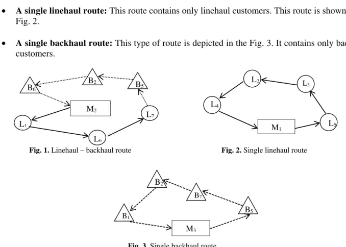
Let us define the total number of depots as m: i.e., �1,�2. . .��, the total number of linehaul customers as ��: �1,�2, … ,��� and the number of backhaul customers as ��: �1,�2, … ,���. The proposed algorithm performs the following routes for a system with three (3) depots: M1. M2 and M3; with seven (7) linehaul customers: �1,�2,�3,�4,�5,�6and �7; and seven (7) backhaul customers: B1, B2, B3, B4, B5, B6and B7:
• A linehaul – backhaul route: The Fig. 1 describes this type of route. Its main feature is that the linehaul and the backhaul sequences are reaching the capacity of the vehicle.
• A single linehaul route: This route contains only linehaul customers. This route is shown in the Fig. 2.
• A single backhaul route: This type of route is depicted in the Fig. 3. It contains only backhaul customers.
Fig. 1. Linehaul – backhaul route Fig. 2. Single linehaul route
Fig. 3. Single backhaul route
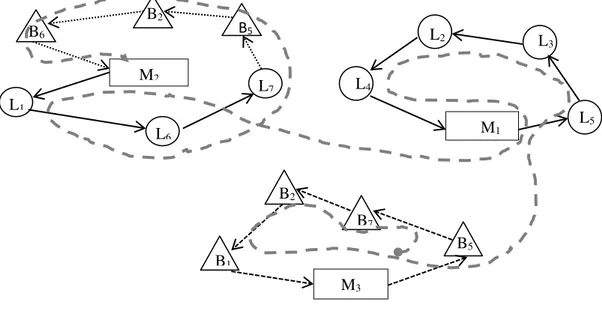
An alternative of solution is conformed by a combination of the three described types of routes. In the proposed algorithm, the construction of a multi-depot solution requires that an ant performs as many subroutes as needed to visit all the customers, and each sub-route comprises a tour considering linehaul and backhaul customers. A possible alternative of solution is shown in the Fig. 4. The dashed line represents the entire tour performed by an ant.
2 M 1
L
6 L
7 L 6
B B2 B5
1
M L5
3
L 2
L
4 L
3 M
5 B
7
B 2
B
1
Fig. 4. Alternative route 3.2 Decision rule
Given the pheromone information, the set of objectives �= {1,2, . . ,�} and the set of all the feasible edges to be selected Ω(�,�) = {(�,�)∈ �}; the edge to be added to the current route performed by an ant is selected according to the following pseudo-random-proportional rule:
(�,�) =
⎩ ⎪ ⎨ ⎪ ⎧
max
(�,�)∈Ω(�)��� ����� �
�=1
�
∝
. ����� ���< �0,
(�,�)
������, ��ℎ������
(8)
where � is a random number between [0,1), �0 is a given parameter between [0,1) representing the probability to select the best next edge, and (�������,�) is the edge to be selected according to the Eq. (4).
3.3 Encoding Solution
Fig. 5 shows the structure used for the distance, time and energy matrices. In particular, we have used a three-dimensional array with dimensions (�+ 1) × (�+ 1) × (�) for each depot. For each matrix, each element ��� corresponds to the distance, the traveling time or the energy of the edge (�.�).
Fig. 5. Encoding for the distance, traveling time and energy matrices
∞ �12 �13 �1� …. �1�+1
�2�+1
���+1
∞
�12 �13 �1� …. �1�+1
�2�+1
���+1
∞ ∞
∞ �12 �13 …. �1� …. �1�+1
�21 ∞ �12 …. �1� …. �2�+1
��1 ��2 ∞ …. ��� …. ���+1
��2
��+1 ��3 …. ��� …. ∞
Depot 1 Depot 2
Depot M
2 M 1
L
6 L
7 L 6
B
2 B
5 B
1 M
L5
3 L 2
L
4 L
3 M
7 B 2
B
1 B
The Visibility Matrix (Fig. 6) is obtained from each element of the matrix elements of distance, time and energy. It contains the inverse matrix of the distance, time and energy. This matrix is symmetrical and is not modified during the execution of the algorithm.
Fig. 6. Encoding of the Visibility matrix
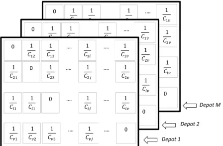
Finally, we proceed to generate the pheromone matrix (Fig. 7) with all positions initialized with the same amount of pheromone. The values of the pheromone matrix are generated with the Eq. (7), and the updating process is restricted to thus elements in the route traveled by each ant.
Fig. 7. Encoding the pheromone matrix
The proposed algorithm avoids flow between depots. Therefore, distance, time and energy among depots are not considered. Indeed, the proposed approach uses a new vehicle to continue visiting other customers. The visibility matrix or net matrix is replaced by a squared array of random values that provides diversity in the searching of the new depot to be added to the current solution. The total number of depots gives the dimension of the visibility matrix, and its values are initialized using the Eq. (7). The nodes are updated only if they belonging to the route traveled by a vehicle. In addition, a vector of not visited customers is required. It contains the feasible customers to be selected.
The solution vector is also required. Its first element is the number of a depot, which is randomly selected. It is followed by a sequence of customer until a new depot has been selected again. However, for each sequence of customers, a Linehaul customer must not appear between two Backhaul customers, and vice versa. The Figure 8 shows an example of a route of the proposed solution.
0 1 �1� 1 �1� 1 �1� 1 �1� …. 1 �2� 1 ��� 0 1 �12 1 �13 1 �1� 1 �1� …. 1 �2� 1 ��� 0 0 0 1 �12 1 �13 1 �1� …. 1 �1� …. 1 �21 0 1 �23 1 �2� …. 1 �2� …. 1 ��1 1 ��1 0 1 ��� …. 1 ��� …. 1 ��2 1 ��1 1 ��3 1 ���
…. …. 0
Depot 1 Depot 2
Depot M
0 �12 �13 �1� …. �1�
�2�
���
0
�12 �13 �1� …. �1�
�2�
���
0 0
0 �12 �13 …. �1� …. �1�
�21 0 �23 …. �1� …. �2�
��1 ��2 0 …. ��� …. ���
��2
��1 ��3 …. ��� …. 0
Depot 1 Depot 2
M2 L1 L6 L7 B5 B1 B6 M2 M1 L4 L2 M1 M3 B4 B3 B2 B7 M3
Linehaul-Backhaul route Linehaul route Backhaul route
Fig. 8. Encoding the solution Vector 3.4 Pseudocode for the proposed algorithm
Procedure PACO-MDVRPB (depots. customers. vehicleNumber. vehicleCapacity)
Initialization of PACO-MDVRPB; /* Generate � ants, Initialize the Pheromone matrixes Calculate Distance, Time and Energy Matrices
Initialize Net Matrices
Initialize Pheromone Contribution Array Initialize Net Contribution Array
Iterations = 0
while iterations < 100 do ants = 0
create �empty routes
determine the objective weigh (��) for each objective � randomly while ants < � do
// Starting MDVRPB procedure initialDepot = choose(depots)
If anyLinehaul(customers) then Process Linehaul customers If anyBackhaul(customers) then Process Backhaul customers select an edge (�,�) by using equation (8)
evaporate(pheromones) update(pheromones) ants++
End while End while 4. Computational results
The proposed approach has been tested on an adapted benchmarking set, which is available in
http://unilibrepereira.edu.co/backhauls/. In particular, 33 benchmarking instances are used to test the effectiveness of the proposed approach. The proposed algorithm has been implemented in MatLab, and computational experiments have been run on a PC with Core i5 1.4 GHz processor and 8GB of RAM. The algorithm has been executed for 10 runs over 100 iterations, reporting the average results and the best results of all runs.
The parameters used to execute the complete set of instances are the following: Iterations =100, α = 1, β
= 3, ρ = 0.01, and the contribution factor of the visited edge = Number of customers / Best solution found
so far.
4.1 Description of the Instances
The matrices of energy have been performed as follows: We have defined three types of vehicles depending of the load (Type 1-T1 with less than 10 ton, Type 2-T2 between 10 and 20 ton, and Type 3-T3 between 20 and 35 ton). The parameters of the frontal area of each vehicle, weigh of the vehicle, weigh of the load, values of �� and �� are described in Table 1.
Table 1
Energy parameters (Source: http://www.kenworthcolombia.com/)
Type 1-T1 Type 2-T2 Type 3-T3
Frontal Area (m2) 7 9 11.44
Weight of the vehicle (kg) 6000 16000 17000
Weight of the load (kg) 10000 20000 35000
�� 0.76 0.85 0.95
�� 0.01 0.0125 0.015
In addition, the following parameters are considered to obtain the energy matrices: acceleration = 0 m/s2, gravity = 9.807, angle of the road = 0o, air density at 20oρ = 1.2041 kg / m3. Finally, the distances and
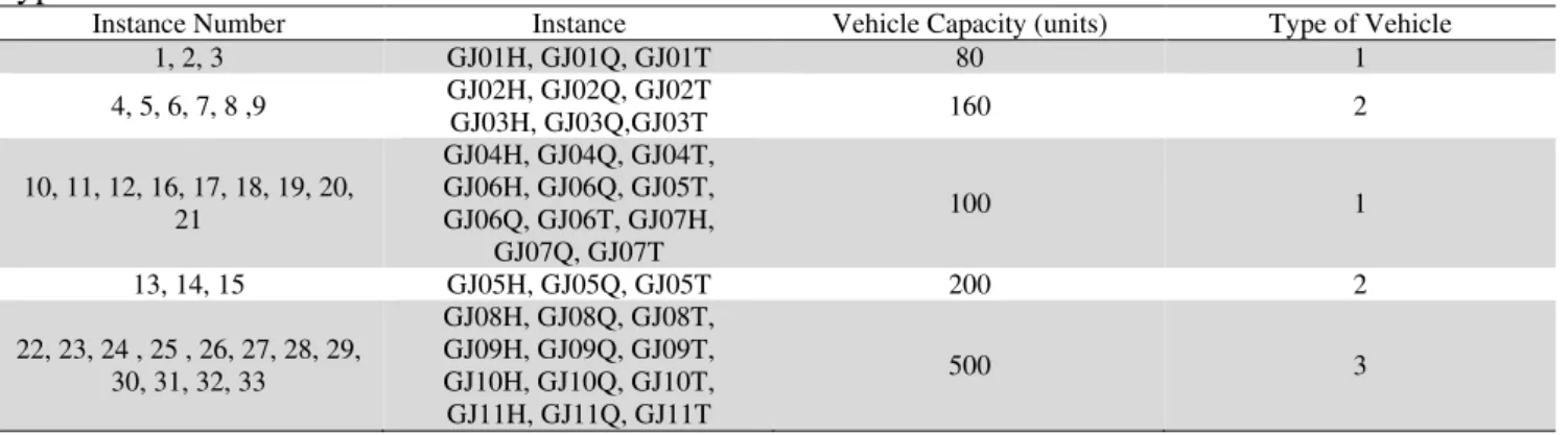
the speed for each edge are calculated with the coordinates � and � and the matrices of traveling time. Table 2 shows the type of vehicle used for each instance.
Table 2
Type of used vehicle for each instance
Instance Number Instance Vehicle Capacity (units) Type of Vehicle
1, 2, 3 GJ01H, GJ01Q, GJ01T 80 1
4, 5, 6, 7, 8 ,9 GJ02H, GJ02Q, GJ02T
GJ03H, GJ03Q,GJ03T 160 2
10, 11, 12, 16, 17, 18, 19, 20, 21
GJ04H, GJ04Q, GJ04T, GJ06H, GJ06Q, GJ05T, GJ06Q, GJ06T, GJ07H,
GJ07Q, GJ07T
100 1
13, 14, 15 GJ05H, GJ05Q, GJ05T 200 2
22, 23, 24 , 25 , 26, 27, 28, 29, 30, 31, 32, 33
GJ08H, GJ08Q, GJ08T, GJ09H, GJ09Q, GJ09T, GJ10H, GJ10Q, GJ10T, GJ11H, GJ11Q, GJ11T
500 3
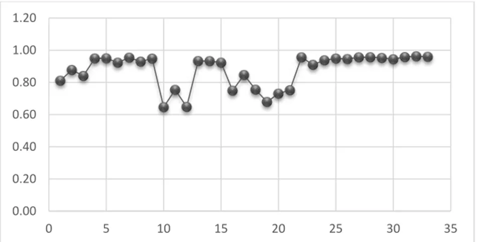
In addition, the correlation of the objectives for each instance is calculated in order to justify the consideration of the three objectives at the same time. As an example, Fig. 9, Fig. 10 and Fig. 11 show the correlation of the three objectives for instance 3. Note that there are low correlations factors for the considered objectives. Therefore, the objectives are independent and a Pareto Front must be calculated.
Fig. 9. Correlation between Distance and Time Fig.10. Correlation between Time and Energy
-0.10 0.00 0.10 0.20 0.30 0.40 0.50 0.60 0.70 0.80 0.90
0 10 20 30 40 -0.60
-0.40 -0.20 0.00 0.20 0.40 0.60
Fig. 11. Correlation between Distance and Energy 4.2 Obtained Results
We report the computing time and the values reached by the metaheuristic objective proposed
Table 3
Obtained results over 10 executions with 100 iterations of the proposed algorithm
Instance Number Instance
Proposed Methodology with PACO – Distance
Proposed Methodology with PACO – Time
Proposed Methodology with PACO – Energy Best Solution Distance (km) Objective Function Time (min) Objective Function Energy (kw/h) Computing Time Objective Function Distance (km) Best Solution Time (min) Objective Function Energy (kw/h) Computing Time Objective Function Distance (km) Objective Function Time (min) Best Solution Energy (kw/h) Computing Time
(sec) (sec) (sec)
1 GJ01H 674.6 828.9 449.5 3.57 804.6 716 646.6 2.64 675.7 833.7 446.2 2.46 2 GJ01Q 776.5 868.9 528.9 3.33 865.1 790.6 669.5 2.49 802.1 977.8 512.9 2.42
3 GJ01T 762.6 848.9 533.2 2.9 886.4 751.7 728 1.38 771.5 922.9 522.1 1.56
4 GJ02H 639.4 675.8 1034 1.06 739.6 651.7 1280.4 1.73 651.8 732.3 1022.7 0.75 5 GJ02Q 675.9 681.3 1136.2 1.31 745.4 646.8 1319.5 2.02 676.7 754.5 1081.3 1.02 6 GJ02T 678.2 698.6 1124.4 2.4 744.2 632.8 1314.8 2.57 680.7 743.7 1077.2 1.57 7 GJ03H 836.5 969 1322.5 4.82 858.8 820.3 1465.1 4.36 840.3 982.2 1321.2 2.05 8 GJ03Q 929 994.7 1499.2 3.29 984.4 907.2 1692.4 6.16 948.9 1150.1 1463.1 3.7 9 GJ03T 909.5 1060.1 1416.1 5.65 956.4 911.6 1645.4 6.61 916 1096.7 1409.9 2.87 10 GJ04H 1203 1307.3 845.6 3.46 1360.5 1170.4 1109.7 2.7 1226.5 1536.7 778.6 3.94 11 GJ04Q 1287.2 1492.1 870.2 2.93 1439.2 1357.4 1116.3 2.76 1312.8 1647.9 840.5 0.98 12 GJ04T 1269.3 1515.5 848 1.41 1391.8 1258.2 1087.8 3.6 1276.2 1563.2 835.8 1.36 13 GJ05H 992.4 1055.2 1639.9 1.62 1096.1 987.7 1909.7 2.14 1024.5 1195.7 1619.9 2.05 14 GJ05Q 1063.5 1245.1 1664.2 3.19 1124.5 1083.9 1901 1.71 1076.3 1303.6 1656.7 1.8 15 GJ05T 1026.8 1035.9 1710.9 4.51 1100.7 963.4 1930.9 1.86 1059.9 1252.6 1664.2 3.28 16 GJ06H 1148.1 1199.6 838.4 4.63 1268.2 1120.9 1011.9 3.12 1222 1564.2 770 3.79 17 GJ06Q 1205.6 1223 878.7 6.73 1269.3 1117.2 1011.4 5.8 1301.2 1540 867.6 3.53 18 GJ06T 1203 1423.4 803.1 6.65 1274 1207.6 963.6 3.71 1240.7 1576 784.7 3.28 19 GJ07H 1100.6 1142.7 808.6 6.32 1231.9 1070.6 995.3 4.75 1144.4 1445 736.6 2.74 20 GJ07Q 1198.6 1392.4 817.9 8.64 1332.7 1151.6 1083.7 4.33 1200.4 1397.7 807.2 5.69 21 GJ07T 1196 1364.4 824.3 7.86 1315.1 1174.6 1049.4 4.91 1200.3 1524.9 758.9 6.68 22 GJ08H 5114.7 5933.9 13481.2 11 5432 4858.5 15515.4 13.88 5154.8 6091.3 13457.3 6.9 23 GJ08Q 5763.4 5835.7 15757.3 20.36 6119.5 5473.9 17584.9 18.8 5904.2 6819.7 15527.1 14.38 24 GJ08T 5879 5779.8 16475.1 24.54 5984.5 5593 17030.9 13.42 5936.9 6953.6 15472.4 13.42 25 GJ09H 5106.8 5624.9 13805.7 13.9 5160.7 4707.6 14694.2 12.53 5112.1 5665.7 13802.7 9.3 26 GJ09Q 5889.9 6279.6 16017.6 11.45 6571.8 5759.2 19018.3 12.2 5906.8 6365 15968 10.99 27 GJ09T 6135.2 6955.2 16281.4 15.31 6505.4 6152.4 18347.4 15.68 6325.3 7989.1 16064 10.28 28 GJ10H 4814.2 5458.5 12859.8 18.14 4888.1 4749 13759.5 21.65 4959.8 5865.1 12808.1 17.03 29 GJ10Q 5387.3 5727.3 14550.6 24.91 6274.3 5434.1 18245.8 30.17 5596.6 6732.9 14453.3 28.9 30 GJ10T 5305.4 5914 14201.1 55.1 5458.3 5249.7 15321.9 27.53 5379.6 6535 13896.9 33.05 31 GJ11H 4725.9 5226.8 12664 28.01 5286.7 4768.7 15107.8 25.88 4725.9 5226.8 12664 24.59 32 GJ11Q 5279.7 5716.9 14208.3 57.18 5882.5 5293.2 16788.1 50.16 5366.7 6500.5 13804.1 22.91 33 GJ11T 5149.7 5577.4 13862.7 47.72 5629.9 5040 16203.9 50.63 5184.4 5836.2 13715.6 18.85
Average 2585.7 2532.5 5836.7
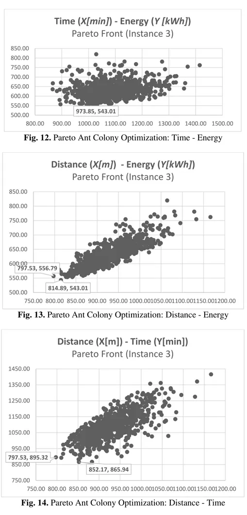
Fig. 12, Fig. 13 and Fig. 14 show the results found for the instance 3 of the Pareto Fronts by using the criterion Min – Min. Note that each figure shows the extreme values of each Pareto Front.
0.00 0.20 0.40 0.60 0.80 1.00 1.20
Fig. 12. Pareto Ant Colony Optimization: Time - Energy
Fig. 13. Pareto Ant Colony Optimization: Distance - Energy
Fig. 14. Pareto Ant Colony Optimization: Distance - Time
973.85, 543.01 500.00
550.00 600.00 650.00 700.00 750.00 800.00 850.00
800.00 900.00 1000.00 1100.00 1200.00 1300.00 1400.00 1500.00
Time (
X[min]
) - Energy (
Y [kWh]
)
Pareto Front (Instance 3)
814.89, 543.01 797.53, 556.79
500.00 550.00 600.00 650.00 700.00 750.00 800.00 850.00
750.00 800.00 850.00 900.00 950.00 1000.001050.001100.001150.001200.00
Distance (
X[m]
) - Energy (
Y[kWh]
)
Pareto Front (Instance 3)
852.17, 865.94 797.53, 895.32
750.00 850.00 950.00 1050.00 1150.00 1250.00 1350.00 1450.00
750.00 800.00 850.00 900.00 950.00 1000.001050.001100.001150.001200.00
Distance (X[m]) - Time (Y[min])
5. Concluding remarks
Multi-objective combinatorial techniques play a decisive role in the field of the vehicle routing problems. Recent researchers have proposed several approaches to solve several variants of the multi-objective vehicle routing problems classified as NP-hard problems.
In this paper, an effective Pareto Ant Colony Optimization has been used to provide an efficient approach for the Multi-objective Multi-Depot Vehicle Routing Problem with Backhauls (MDVRPB). In particular, three objectives of traveled distance, traveling times and total consumption of energy have been minimized. In addition, we have used multiple pheromone matrices and random weights for each objective. The performance of the proposed algorithm has been evaluated by considering adapted instances from the literature.
The proposed methodology could be extended to other vehicle routing problems with many or few constraints and/or objectives. In addition, new heuristic information could be added easily to the proposed approach. We suggest proving the proposed approach to other routing problems such as the Multi Depot Vehicle Routing Problem (MDVRP), the Periodic Location Routing Problem (PLRP), the Muti-Depot Vehicle Routing Problem with Heterogeneous Fleet (HMDVRP), among others.
References
Anbuudayasankar, S. P., Ganesh, K., Koh, S. L., & Ducq, Y. (2012). Modified savings heuristics and genetic algorithm for bi-objective vehicle routing problem with forced backhauls. Expert Systems with
Applications, 39(3), 2296-2305.
Bektaş, T., & Laporte, G. (2011). The pollution-routing problem. Transportation Research Part B:
Methodological, 45(8), 1232-1250.
Bolaños, R., Echeverry, M., & Escobar, J. (2015). A multiobjective non-dominated sorting genetic algorithm (NSGA-II) for the Multiple Traveling Salesman Problem. Decision Science Letters, 4(4), 559-568.
Chunyu, R., Zhendong, S., & Xiaobo, W. (2009, June). Study on single and mixed fleet strategy for multi-depot vehicle routing problem with backhauls. In Computational Intelligence and Natural
Computing, 2009. CINC'09. International Conference on (Vol. 1, pp. 425-428). IEEE.
Chunyu, R., & Xiaobo, W. (2009, October). Study on hybrid genetic algorithm for multi-type vehicles and multi-depot vehicle routing problem with backhauls. In Intelligent Computation Technology and
Automation, 2009. ICICTA'09. Second International Conference on (Vol. 1, pp. 197-200). IEEE.
Demir, E., Bektaş, T., & Laporte, G. (2014). The bi-objective pollution-routing problem. European
Journal of Operational Research, 232(3), 464-478.
Doerner, K., Gutjahr, W. J., Hartl, R. F., Strauss, C., & Stummer, C. (2004). Pareto ant colony optimization: A metaheuristic approach to multiobjective portfolio selection. Annals of Operations
Research, 131(1-4), 79-99.
Escobar, J. W., Linfati, R., & Toth, P. (2013). A two-phase hybrid heuristic algorithm for the capacitated location-routing problem. Computers & Operations Research, 40(1), 70-79.
Escobar, J. W., Linfati, R., Toth, P., & Baldoquin, M. G. (2014a). A hybrid granular tabu search algorithm for the multi-depot vehicle routing problem. Journal of Heuristics, 20(5), 483-509.
Escobar, J. W., Linfati, R., Baldoquin, M. G., & Toth, P. (2014b). A Granular Variable Tabu Neighborhood Search for the capacitated location-routing problem. Transportation Research Part B:
Methodological, 67, 344-356.
Escobar, J. W., Linfati, R., & Adarme-Jaimes, W. (2015). A hybrid metaheuristic algorithm for the capacitated location routing problem. Dyna, 82(189), 243-251.
Gutjahr, W. J. (2002). ACO algorithms with guaranteed convergence to the optimal solution. Information
Processing Letters, 82(3), 145-153.
Jozefowiez, N., Semet, F., & Talbi, E. G. (2008). Multi-objective vehicle routing problems. European
Journal of Operational Research, 189(2), 293-309.
Lau, H. C., Chan, T. M., Tsui, W. T., Chan, F. T., Ho, G. T., & Choy, K. L. (2009). A fuzzy guided multi-objective evolutionary algorithm model for solving transportation problem. Expert Systems with
Applications, 36(4), 8255-8268.
Liu, C. M., Chang, T. C., & Huang, L. F. (2006). Multi-objective heuristics for the vehicle routing problem. International Journal of Operations Research, 3(3), 173-181.
Min, H., Current, J., & Schilling, D. (1992). The multiple depot vehicle routing problem with backhauling. Journal of Business Logistics, 13(1), 259.
Mohammadi, M., Tavakkoli-Moghaddam, R., & Rostami, R. (2011). A multi-objective imperialist competitive algorithm for a capacitated hub covering location problem. International Journal of
Industrial Engineering Computations, 2(3), 671-688.
Mortezaei, M., & JabalAmeli, M. (2011). A hybrid model for multi-objective capacitated facility location network design problem. International Journal of Industrial Engineering Computations, 2(3), 509-524.
Nezhad, A., Roghanian, E., & Azadi, Z. (2013). A fuzzy goal programming approach to solve multi-objective supply chain network design problems. International Journal of Industrial Engineering
Computations, 4(3), 315-324.
Rao, R., & Patel, V. (2014). A multi-objective improved teaching-learning based optimization algorithm for unconstrained and constrained optimization problems. International Journal of Industrial Engineering Computations, 5(1), 1-22.
Ropke, S., & Pisinger, D. (2006). A unified heuristic for a large class of vehicle routing problems with backhauls. European Journal of Operational Research, 171(3), 750-775.
Salhi, S., & Nagy, G. (1999). A cluster insertion heuristic for single and multiple depot vehicle routing problems with backhauling. Journal of the Operational Research Society, 50(10), 1034-1042.
Wade, A., & Salhi, S. (2001, July). An ant system algorithm for the vehicle routing problem with backhauls. In MICÕ2001––4th Metaheuristic International Conference.
Wade, A., & Salhi, S. (2004). An ant system algorithm for the mixed vehicle routing problem with
backhauls. In Metaheuristics: computer decision-making (pp. 699-719). Springer US.
Yalcın, G. D., & Erginel, N. (2015). Fuzzy multi-objective programming algorithm for vehicle routing
problems with backhauls. Expert Systems with Applications, 42(13), 5632-5644.
Yazdian, S., & Shahanaghi, K. (2011). A multi-objective possibilistic programming approach for locating distribution centers and allocating customers demands in supply chains. International Journal of
Industrial Engineering Computations, 2(1), 193-202.