Homogenization of a Continuously Microperiodic Multidimensional Medium

doi: 10.5540/tema.2018.019.01.0015

Homogenization of a Continuously Microperiodic

Multidimensional Medium

M. P. LIMA1*, L. D. P ´EREZ-FERN ´ANDEZ2and J. BRAVO-CASTILLERO3

Received on November 19, 2016 / Accepted on March 11, 2018

ABSTRACT. The asymptotic homogenization method is applied to obtain formal asymptotic solution and the homogenized solution of a Dirichlet boundary-value problem for an elliptic equation with rapidly os-cillating coefficients. The proximity of the formal asymptotic solution and the homogenized solution to the exact solution is proved, which provides the mathematical justification of the homogenization pro-cess. Preservation of the symmetry and positive-definiteness of the effective coefficient in the homogenized problem is also proved. An example is presented in order to illustrate the theoretical results.

Keywords: Microperiodic medium, effective behavior, asymptotic homogenization method.

1 INTRODUCTION

The heterogeneous medium is formed by distributions of occupied domains: (a) by different ho-mogeneous materials called phase, thus constituting a composite; or (b) of the same material in different states, such as a polycrystal [21], or a functionally graded material [19]. Heteroge-neous medium abound in nature and in manufactured products. For example: among the natural medium that have heterogeneity are the bone, atmosphere, soil, sandstone, wood, lungs, veg-etable and animal tissues, cell aggregates, tumors; (solid, granular or particulate, fibrous, and combinations thereof), and cell solids, gels, foams, metal alloys, microemulsions, ceramic and block copolymers [21]. The theoretical prediction of mechanical, electromagnetic, and transport properties of heterogeneous materials has a long and venerable history, attracting the attention of science icons, including Maxwell [14], Rayleigh [18] and Einstein [10]. Generally, the physical phenomena of interest associated with such properties occur in the ”microscale”, called generi-cally so, because it can be in the order of tenths of nanometers (gels) up to the order of meters (geological processes). Such medium exhibit separation of structural scales, which is character-ized by the small parameterε=l/L, 0<ε≪1, wherelandLare, respectively, the characteristic

*Corresponding author: Marcos Pinheiro de Lima – E-mail: marcos.lima@ufrgs.br. 1Universidade Federal do Rio Grande do Sul, Brazil.

2Universidade Federal de Pelotas, Brazil. E-mail: leslie.fernandez@ufpel.edu.br

lengths of the micro- and macroscale. Also, these medium are assumed to satisfy the continuum hypothesis, that is,lis much greater than the characteristic length of the molecular scale. With such assumptions, micro-heterogeneous medium are regarded as a continuum at the microscale, so they can be characterized via effective properties [21]. More precisely, the hypothesis of equiv-alent homogeneity states that, at the macroscale, an heterogeneous medium is physically equiva-lent to an ideally homogeneous medium in such a way that the effective properties of the former are the properties of the latter [2]. The process of obtaining the effective behavior of micro-heterogeneous medium is called homogenization. The periodicity is characterized by periodic replication of a recurrent elementY called basic cell.

Phenomena occurring within a micro-heterogeneous medium are described by initial/boundary-value problems whose differential equations have rapidly oscillating coefficients, whereas the equations of the problems for the equivalent homogeneous medium have constant coefficients [2]. Thus, the hypothesis of equivalent homogeneity will be valid if the solutionuεof a problem for the heterogeneous medium is ε-near of the solution u0 of the problem for the equivalent homogeneous medium with respect to some norm, that is,kuε₋u0k=O(ε).

We can find various applications of homogenization theory in literature, for example: obtaining properties coupled nonexistent in the constituents (magnetoelectric [4], pyroelectric and pyro-magnetic [5]); topology optimization [3]; optimal design of heterogeneous materials [22]; biome-chanics of bone [16], prediction of structural failures [17]; propagation of seismic waves [7]; physics of nuclear reactors [1]; transport of a chemical species [15].

In this contribution, we study the following elliptic problem: Finduε_∈C2(Ω),Ω= [0,1]d_{, such}

that

Lε_uε_≡ ∂ ∂xj

aε_jl(x)∂u

ε

∂xl

=f(x),x_∈Ω, uε=0,x_∈∂Ω, (1.1)

where, j,l=1,2, ...,d,aε_jl∈C1(Ω)areεY-periodic,Y= [0,1]d_{, symmetric and positive-definite,}

that is,aε_jl(x) =aε_{l j}(x)for all x_∈Ω (symmetry) and∀η∈Rd_,∃c>0 :∀x_∈Rd_,aε_jl(x)ηjηl≥

cηlηl(positive definiteness), respectively. In (1.1), and throughout the work, Einstein’s notation

for the sum over repeated indexes is adopted.

Problem (1.1) models, for instance, the distribution of a stationary temperature fielduε over a periodic micro-heterogeneous conductive medium with thermal conductivityaε_jl(x) =ajl(x/ε)in

the presence of a distributed heat sourcef. Notice that this problem is, in general, hard of to solve analytically, while a direct numerical approach requires a very fine discretization of the domain in order to capture the rapidly oscillating behavior of the coefficients aε_jl(x), which increases considerably the computational cost and compromises the convergence of the adopted numeric method. An effective and mathematically rigorous alternative is the Asymptotic Homogenization Method (AHM) [2]. The AHM proposes a formal asymptotic solution (f.a.s.) of the original problem (1.1), that is, a two-scale asymptotic series of powers ofε,

u(∞)(x,ε) =

∞

∑

εiui(x,y), y=

x

Note that, asLε_{is a linear operator, the asymptotic series (1.2) is also an asymptotic expansion} of the exact solution of the problem:uε _∼u(∞). The unknown coefficientsui∈C2(Ω×Rd)of

the powers ofε, which areY-periodic functions with respect to the so-called local variabley, are obtained as the solutions of a recurrent sequence of problems which results from subsituting (1.2) into the original problem (1.1).

The work is structured as follows: in section 2, we develop the AHM in detail to build the f.a.s.; in section 3, we mathematically justify the AHM, i.e., we prove thatkuε₋u0k_H1

0(Ω)=

O₍p_ε),

whereH₀1(·)is the space of null-trace square-integrable functions whose generalized first-order derivatives are square-integrable; in sections 4 and 5, we show some properties preserved on apply of the AHM; an example is solved in section 6, showing the development analytical (sep-aration of variables) and numerical (finite difference method) applied; finally, in section 7 we describes the conclusions about development realized in the previous sections.

2 APLICATION OF THE AHM

Following [2], consider the f.a.s

u(2)(x,ε) =u0(x,y) +εu1(x,y) +ε2u2(x,y), y=

x

ε, (2.1)

for problem (1.1). By substituting (2.1) into the equation of (1.1), applying the chain rule

∂Ψε

∂xj

=∂Ψ

∂xj

+1

ε ∂Ψ

∂yj

y=x/ε

,

whereΨε=Ψ(x,xε), and grouping by powerε, we have

Lεu(2)₋f(x) =ε−2_L

yyu0+ε−1(Lxyu0+Lyxu0+Lyyu1)

+ε0_(L

xxu0+Lxyu1+Lyxu1+Lyyu2−f(x)) +O(ε), (2.2)

where the differential operatorsL_{αβ,α,β∈ {x,y}, are defined as}

L_αβ≡ ∂ ∂ αj

ajl(y)

∂ ∂ βl

.

Thus, in order tou(2)given by (2.1) be a f.a.s of problem (1.1), that is, for the right-hand side of (2.2) be assimptotically null, its unknown coefficientsuimust satisfy the following recurrent

equations:

ε−2 : L_{yyu0=0 (2.3)}

ε−1 : L_yyu1=−L_xyu0−L_{yxu0 (2.4)}

ε0 : L_yyu2=−L_xxu0−L_xyu1−L_{yxu1+f(x). (2.5)}

Lemma 1.Let ajl(y)and F(y)be Y -periodic differentiable functions, such that ajl(y)is

symmet-ric and positive definite. Then, a necessary and sufficient condition for a Y -periodic solution of the equation

L_yyN≡ ∂ ∂yj

ajl(y)

∂N ∂yl

=F(y), (2.6)

to exist is that F(y)has null mean value, that is,

hF(y)i ≡

Z

YF(y)dy=0,

where_h·iis the local averaging operator over the periodic cell.

Remark 2.Note that the Y -periodic solution N of (2.6) is unique up to an additive constant, that is, N(y) =N(y) +e C, whereN(y)e is the null-average Y -periodic solution of (2.6),_hNe_i=0, and C is an arbitrary constant.

Remark 2 of Lemma 1 applied to (2.3) implies thatu0does not depend ony:

u0(x,y) =u0(x). (2.7)

By substituting (2.7) into (2.4), we have

L_yyu1=−L_{yxu0, (2.8)}

which, by applying Lemma 1, implies that there existsu1,Y-periodic solution of (2.8), asajl(y)

isY-periodic, soh∂ajl/∂yji=0. In order to solve (2.8), we seek its solutionu1by separation of variables as

u1(x,y) =Np(y)

∂u0

∂xp

. (2.9)

Substitution of (2.9) into (2.8) yields

∂ ∂yj

ajl(y)

∂Np

∂yl

∂u0

∂xp

=−∂_∂ajl yj

∂u0

∂xl

, (2.10)

which, by replacing the indexlbypin the right-hand side, leads to

∂ ∂yj

aj p(y) +ajl(y)

∂Np

∂y_l

∂u0

∂xp

=0. (2.11)

Assume that ∂u0/∂xp6=0. Then, (2.11) is satisfied by Np(y), p =1, . . . ,d, the Y-periodic

solutions of the so-called local problems:

∂ ∂yj

aj p(y) +ajl(y)

∂Np

∂yl

=0, y_∈Y, hNp(y)i=0. (2.12)

Lemma 1 guarantees the existence of Np(y), Y-periodic solutions of LyyNp=F with F =

Application of Lemma 1 provides a necessary and sufficient condition for the existence ofu2,

Y-periodic solution of (2.5):

hL_xxu0+L_xyu1+L_{yxu1i −f(x) =0. (2.13)}

Substitution of (2.9) into (2.13) followed by the appropriate index replacement yields _∂

∂yl

al j(y)Np(y)

+ajl(y)

∂Np

∂yl

+aj p(y) _∂2_u

0

∂xj∂xp

=f(x). (2.14)

Notice that,∂ al j(y)Np(y)

/∂yl

=0, asaj p(y)andNp(y)areY-periodic. Thus, (2.14) can be

rewritten as

b

aj p

∂2_u 0

∂xj∂xp

=f(x), (2.15)

which is the equation of the so-called homogenized problem, and

b

aj p=

ajl(y)

∂Np

∂y_l +aj p(y)

(2.16)

are the so-called effective coefficients. The homogenized problem is defined as: findu0∈C2(Ω) such that

b

aj p

∂2_u 0

∂xj∂xp

=f(x),x_∈Ω, u0(x) =0, x∈∂Ω (2.17)

whereabj pare the effective coefficients given by (2.16). Also, notice that the existence ofu0(x) solution of (2.17) guarantees the existence ofu2(x,y)Y-periodic solution of (2.5). By substituting (2.9) and (2.15) into (2.5), we have

L_yyu2=−

∂ ∂yl

a_{l j}(y)Np(y)

+ajl(y)

∂Np

∂yl

+aj p(y)−abj p

∂2_u 0

∂xj∂xp .

This show that the solutionu2can be sought as

u2(x,y) =Npq(y)

∂2_u 0

∂xp∂xq

, (2.18)

whereNpq(y)is theY-periodic solution of the so-called second local problem, which is obtained

by substituting (2.15) and (2.18) into (2.5) and following the same steps as for obtainingu1. The second local problem is

L_{yyNpq=abpq−Tpq,y∈Y, hNpqi=0, (2.19)}

where

Tpq(y) =apq(y) +aql(y)

∂Np

∂y_l + ∂

∂y_l alq(y)Np(y)

.

The existence of theY-periodic solutionNpqof problem (2.19) is guaranteed by Lemma 1.

Finally, the second-order f.a.s.u(2)(x,ε)of the original problem (1.1) is

u(2)(x,ε) =u0(x) +εNp _x

ε

_∂u0

∂xp

+ε2_N pq

_x

ε

_∂2_u 0

∂xp∂xq

On the other hand, we show in the next section that the first-order f.a.su(1)(x,ε)consisting of the two first terms ofu(2)(x,ε)in (2.20) yields a good approximation of the exact solutionuε(x) of the original problem (1.1).

3 PROXIMITY

In general, the f.a.su(2), constructed to approximate the exact solutionuεof the original problem (1.1), does not satisfy the boundary conditionuε_|∂Ω=0. As the solutionu0of the homogenized problem (2.17) satisfies the boundary conditionu0|∂Ω=0, it follows that the error ofu(2)|∂Ω is nonzero of orderε. In order to overcome such a situation, we multiplyεu1+ε2u2by a function

χ(x)to force the f.a.s. to satisfy exactly the boundary condition, but this adds some new terms to the error. However, these terms are evaluated as being of order√εin the norm ofH−1_{(Ω), that} is, the error in form f0+∂fi/∂xi, withkf0kL2_(Ω)andkfikL2_(Ω)of order√ε, whereL2(·)is space of square-integrable functions, so we can apply an estimate for the solution inH₀1(Ω).

Specifically, ifNpare solutions of the local problems (2.12),Npqare solutions of the second local

problems (2.19),u0is the solution of the homogenized problem (2.17), andu0(x)∈C2(Ω), then the f.a.s (2.20) is solution of the equation

Lε_u(2)_{−f(x) =εr}(2)_(x,ε)

whereεr(2)_{(x,ε)is the error of takingu}(2)_{as the solution of the original problem:}

εr(2)(x,ε) =ε(L_xyu2+L_yxu2+L_{xxu1) +ε}2L_xxu2,y=x ε.

Notice that, by assuming thatu0∈C4(Ω), the application of Weierstrass theorem [13] ensures thatkr(2)_(x,ε)k

L2_(Ω)=O(1). However, the error ofu(2)in the boundary∂Ωis of orderε:

u(2)_|∂Ω=εu1|∂Ω+ε2u2|∂Ω.

Let χ(x) be an infinitely differentiable function with support contained inside the ε -neighbourhood of∂Ω and such thatχ|∂Ω =1, |χ| ≤1, andkε∂ χ/∂xkC(Ω)≤c1, where c1 is a constant independent ofε.

Consider the modified second-order f.a.s

e

u(2)(x,ε) =u(2)_{(x,ε)−χ(x) εu}

1(x,y) +ε2u2(x,y)

=u0(x) +ε(1−χ(x))u1(x,y) +ε2(1−χ(x))u2(x,y),y=

x

ε (3.1)

that satisfies exactly the boundary conditions of the original problem (1.1). In order to assess how goodue(2)is as an approximation ofuε, we have to estimate the error given by the right-hand side of

Lεu_e(2)₋f(x) =εr(2)_(x,ε)− ∂ ∂xj

where

Φ_j(x,ε) =a_jlx ε

ε∂(χu1) ∂xl

+ε2∂(χu2)

∂xl

. (3.3)

First, by the hypotheses onχ, we have thatΦ_j(x,ε)is such thatΦj(x,ε)

_≤c2for everyx∈Ω, wherec2is a constant independent ofε, and its support is contained inside theε-neighbourhood of∂Ω. For instance, ford=3, we have that

Φj(x,ε) =0,x∈[ε,1−ε]3, (3.4)

andkΦ_j(x,ε)kL2_(Ω)=O(√ε). Indeed, by (3.4) we have that

kΦ_j(x,ε)k2L2_(Ω)=

Z

Ω

Φ2_j(x,ε)dx=

Z

Ω_\[ε,1−ε]3Φ 2

j(x,ε)dx. (3.5)

Consider the domainsΩ∗₌Ω_\[ε,1−ε]3_∋xandΩ∗

ε∋x/εsuch thatΩ∗=εΩ∗ε. By substituting

(2.9) and (2.18) into (3.5) with (3.3), and differentiating, we obtain

Z Ω∗ ajl _x ε

ε∂(χu1) ∂xl

+ε2∂(χu2) ∂xl

2 dx = Z Ω∗ ajl _x ε εNp _x ε _{∂ χ}

∂xl

∂u0

∂xp

+χ(x) ∂

2_u 0

∂xp∂xl

+ε2Npq _x

ε

_{∂ χ}

∂xl

∂2_u 0

∂xp∂xq

+χ(x) ∂

3_u 0

∂xp∂xq∂xl 2

dx.

By Weierstrass theorem, there are constants B0,B1 eB2 such that |ajl| ≤B0,|Np| ≤B1 and

|Npq| ≤B2for everyx/ε∈Ωε∗. By takingB=max{B0,B1,B2}, we have that

Z Ω∗ ajl _x ε

ε∂(χu1) ∂xl

+ε2∂(χu2) ∂xl

2

dx

≤B4

Z

Ω∗

ε_∂∂ χxl

∂ u0

∂xp +ε|χ|

∂ 2_u 0

∂xp∂xl +ε ε∂ χ_∂xl

∂ 2_u 0

∂xp∂xq +ε2|χ|

∂ 3_u 0

∂xp∂xq∂xl 2 dx.

By Weierstrass theorem, there are constantsC0,C1,C2andC3such that

ε

∂ χ ∂xl ≤C0,

∂u0

∂xp ≤C1,

∂2_u 0

∂xp∂xl ≤C2,

∂3_u 0

∂xp∂xq∂xl

≤C3, ∀x∈Ω∗.

By recalling that|χ| ≤1 and takingC=max{1,C0,C1,C2,C3}, we have that

Z Ω∗ ajl _x ε

ε∂(χu1) ∂xl

+ε2∂(χu2) ∂xl

2

dx_≤B4C4(1+ε)4

Z

Ω∗dx.

Then, from (3.5) it follows that

whereD(ε) =3ε−6ε2_+4ε3_{is of orderO(ε). Therefore,}

kΦ_j(x,ε)kL2_(Ω)≤ √

2B2C2(1+ε)2pD(ε),

which proves that_kΦ_j(x,ε)_kL2_(Ω)=O(√ε).

Now, subtracting of the equation of problem (1.1) from (3.2) yields

∂ ∂xj

aε_jl(x) ∂ ∂xl

(ue(2)₋uε)

=εr(2)_(x,ε)− ∂ ∂xj

Φ_j(x,ε),

from which, recalling that(eu(2)₋uε)|∂Ω=0, the maximum principle for elliptic equations [2] provides the estimate

kue(2)₋uε_kH1

0(Ω)≤c3 εkr

(2)_(x,ε)k

L2_(Ω)+ 3

∑

kΦ_j(x,ε)kL2_(Ω) !

, (3.6)

where constantc3is independent ofε. Recall that, foru0∈C4(Ω), we havekr(2)(x,ε)kL2_(Ω)= O_{(1). Then, (3.6) implies that the modified second-order f.a.s (3.1) satisfies the relation}

keu(2)₋uε_kH1 0(Ω)=

O₍√_ε)

and, in particular,

keu(1)₋uε_kH1 0(Ω)=

O₍√_ε),

whereu_e(1)(x,ε) =u(1)₋ε χu1is the related first-order modified f.a.s

Finally, in order to show the proximity betweenu0anduε, it suffices to prove, following the procedure described above, that

keu(1)₋u0kH1 0(Ω)=

O₍√_ε).

Therefore, from the Minkowski inequality’s [11]

kuε₋u0k_H1

0(Ω)≤ ku

ε

−eu(1)_kH1

0(Ω)+kue (1)

−u0k_H1 0(Ω), it follows that

kuε₋u0kH1 0(Ω)=

O₍√_ε).

An alternative approach to estimateuε₋u˜(1)and ˜u(1)₋u0is through an estimative for the so-lution of non homogeneous Dirichlet problem provided in [9]. In that book, such an approach was applied and similar results were obtained, that is, theO₍√_{ε)proximity for homogeneous} boundary condition. Other approaches can be applied to know to proximity between theuεandu0 solutions, for instance, proposes asymptotic expansions of which its coefficients are convolution forms of Green function and the source term of the elliptic equation, so from the representation of the elliptic solution by the Green function, we estimate the proximity of the expansion truncated and the exact solution [8].

4 PRESERVATION OF SYMMETRY

First, observe that the effective coefficients (2.16) can be rewritten as

b

aj p=

akl(y)

∂Mj

∂yk

∂Mp

∂yl

−

akl(y)

∂Nj

∂yk

∂Mp

∂yl

, (4.1)

whereMp=Np+yp. We will show that the first term on the right-hand side of (4.1) is symmetric

with respect to indexes jandp, and that the second term is null.

First, we show that the second term of (4.1) is null. Consider the equation of the local problem (2.12) rewritten as

∂ ∂yj

ajl(y)

∂Mp

∂y_l

=0,y_∈Y.

Letφ=φ(y)beY-periodic and continuously differentiable. Then,

∂ ∂yj

ajl(y)

∂Mp

∂yl

φ(y) =0,y_∈Y, (4.2)

so

∂ ∂yj

ajl(y)

∂Mp

∂y_l φ(y)

=ajl(y)

∂Mp

∂y_l ∂ φ ∂yj .

By applying the average operator, we get

∂ ∂yj

ajl(y)

∂Mp

∂yl

φ(y)

=

ajl(y)

∂Mp

∂yl

∂ φ ∂yj

. (4.3)

Note that Mp is not Y-periodic. However, ∂Mp/∂yl = ∂Np/∂yl+δpl is Y-periodic. So,

φ(y)ajl(y)∂Mp/∂yl isY-periodic, which implies that the term on the left-hand side of (4.3) is

null. Therefore, we have

ajl(y)

∂Mp

∂y_l ∂ φ ∂yj

=0,

for everyY-periodicφ∈C1(Y). In particular, by takingφ=Nk, it follows that

ajl(y)

∂Mp

∂y_l ∂Nk

∂yj

=0. (4.4)

Thus, by putting (4.4) into (4.1), we have

b

aj p=

akl(y)

∂Mj

∂yk

∂Mp

∂yl

. (4.5)

Finally, the symmetry ofabj pfollows from interchanging the indexeskandl, and considering the

symmetry ofalk:

b

aj p=

alk(y)

∂Mj

∂y_l ∂Mp

∂y_k

=

alk(y)

∂Mp

∂y_k ∂Mj

∂y_l

=

akl(y)

∂Mp

∂y_k ∂Mj

∂y_l

=abp j.

Therefore,abj p=abp j, which provides a way to control calculations of the effective coefficients

5 PRESERVATION OF POSITIVE-DEFINITENESS

Preservation of positive-definiteness of the effective coefficients implies that the equation of the homogenized problem is elliptic. Recall from the formulation of the original problem (1.1) that the coefficienta_jl is positive definite, that is,∃c>0, ∀η∈Rd_|a

jl(y)ηjηl≥cηlηl, ∀y∈Y.

In order to show the positive-definiteness ofabj p, a similar relation must be proved. Indeed, it

follows from (4.5) that

b

aj pηjηp=

a_kl(y)∂Mp ∂yk

∂Mj

∂yl

ηjηp=

a_klηp

∂Mp

∂yk

ηj

∂Mj

∂yl

. (5.1)

Asaklis positive-definite, we have

akl(y)ηp

∂Mp

∂yk

ηj

∂Mj

∂yl ≥

c

d

∑

ηj

∂Mj

∂yl 2

,∀y_∈Y. (5.2)

Then, by substitution (5.2) into (5.1), we have

b

aj pηjηp≥c d

∑

*

ηj

∂Mj

∂yl 2+

.

From the Cauchy-Buniakovski inequality [12], we have

b

aj pηjηp≥c d

∑

ηj

∂Mj

∂yl 2

,

which can be rewritten as

b

aj pηjηp≥c d

∑

ηj

∂Nj

∂yl

+

ηj

∂yj

∂yl 2

, (5.3)

where

ηj

∂Nj

∂yl

=0 and

ηj

∂yj

∂yl

=ηjhδjli=ηl.

So, it follows from (5.3) that

b

aj pηjηp≥c d

∑

η2

l =cηlηl,

that is, the effective coefficientabj p is positive-definite, which provides another way to control

calculations ofabj pperformed via other analytical or numerical techniques.

6 EXAMPLE

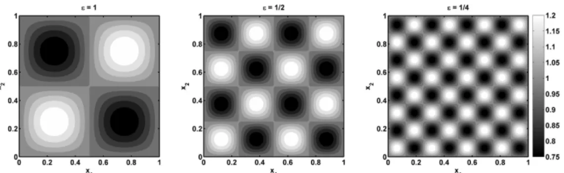
Consider problem (1.1) with the source term f(x) =−1 and isotropic coefficients aε_jl(x) = aε(x)δjl, where aε(x) =1+0.25 sin(2πx1/ε)sin(2πx2/ε). Figure 1 shows the behavior of

Figure 1: Continuously differentiable, positive, bounded and rapidly oscillating coefficients for the three-dimensional elliptic linear problem.

For this problem, we solve the local problem (2.12), obtain the effective coefficients (2.16) and solve the homogenized problem (2.17). Notice that the first of these problems is two-dimensional from the point of view of the homogenization, asajl(y)depend only ony1andy2becauseaε(x) depend only onx1andx2. Therefore, from (2.12), we solve the following local problem:

∂ ∂y1

a(y)∂Np ∂y1

+ ∂

∂y2

a(y)∂Np ∂y2

=−_∂∂_ya

p

, y_∈Y, hNp(y)i=0, (6.1)

for each p=1, 2, 3. The equation in (6.1) is a Poisson equation’s forp=1,2 and a Laplace equation’s forp=3. To solve it, the finite difference method was used [20, 6], which comprises the following steps:

• A mesh of(N+2)2_{nodes for the periodic cellY in they}

1y2-plane is defined. In particular, the local functionsNpare taken to be null on the nodes of∂Y.

• The discretization of the equation in (6.1) on an arbitrary point(y1i,y2j)is

ci,jN_ip₊1,j+di,jN p

i−1,j+ei,jN p

i,j+1+fi,jN_ip_,j−1+gi,jNip,j=F p i,j,

where

ci,j=

a(_i,1_j) 2h +

ai,j

h2,di,j=

ai,j

h2 −

a(_i,1_j) 2h ,ei,j=

a(_i,2_j) 2h +

ai,j

h2, fi,j=

ai,j

h2 −

a(_i,2_j) 2h ,

gi,j=−

ai,j

h2,F 1 i,j=−a

(1)

i,j,F 2 i,j=−a

(2)

i,j,F 3 i,j=0,

a(_i,1_j)= ∂a ∂y1

(y1i,y2j),a (2)

i,j =

∂a ∂y2

(y1i,y2j),

• A system of linear equationsAb=Fpis assembled as follows. TheN2_×N2matrixAis structured in blocks as:

A=             

S1 R1 0 ··· ··· 0

T2 S2 R2 . .. . .. ...

0 T3 S3 R3 . .. ... ..

. . .. ... ... . .. 0

..

. . .. ... TN−1 SN−1 RN−1 0 ··· ··· 0 TN SN

            

N2_×N2

, (6.2)

where{Sj}1≤j≤N,{Rj}1≤j≤N−1and{Tj}2≤j≤N, areN×Nblocks given by:

Sj=             

c1,j d1,j 0 ··· ··· 0

e2,j c2,j d2,j . .. . .. ...

0 e3,j c3,j d3,j . .. ...

..

. . .. ... ... . .. 0

..

. . .. ... eN−1,j cN−1,j dN−1,j

0 _{··· ···} 0 eN,j cN,j             

N×N ,

Rj=             

f1,j 0 0 ··· ··· 0

0 f2,j 0 . .. ... ...

0 0 f3,j 0 . .. ...

..

. . .. ... ... ... 0

..

. . .. ... 0 fN₋1,j 0

0 ··· ··· 0 0 fN,j

            

N×N ,

and

Tj=             

g1,j 0 0 ··· ··· 0

0 g2,j 0 . .. ... ...

0 0 g3,j 0 . .. ...

..

. . .. ... ... ... 0

..

. . .. ... 0 gN−1,j 0

0 ··· ··· 0 0 gN,j

            

N×N .

The vectorbof unknowns in the linear system is defined as:

wherewk,k=1, . . . ,N2are defined asNip,jfori,j=1, . . . ,N. Finally, vectorFpis defined

as:

Fp=hF₁p_,1F₁p_,2...F₁p_,NF₂p_,1F₂p_,2...F₂p_,N...F_Np_,1F_Np_,2...F_Np_,NiT

N2_×1. (6.4)

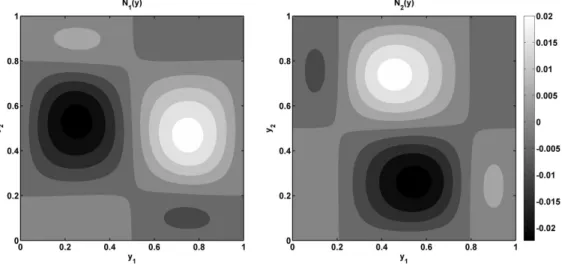
The following results were obtained for a mesh of 10000 nodes, for each p. The full time of this simulation was approximately 100 seconds. Figure 2 shows the solutions Np of the local

problems, forp=1,2, asN3(y) =0.

Figure 2: Solutions of the local problemsN1andN2, beingN3=0.

Notice that the local solutionsNpwere calculated assuming homogeneous Dirichlet conditions

on the boundary of the periodic cell, that is, the condition hNpi=0 in local problem (2.12)

was replaced byNp|∂Y =0, in order to ensure that the first-order f.a.su(1) satisfy exactly the

boundary conditions of the original problem. On the other hand, notice that Lemma 1 uses the null-average condition for uniqueness. In general, different choices of uniqueness conditions on the local solutions will affect the behavior of u(1) only in the neighborhood of the boundary. However, the difference between the local solutions obtained from these different conditions is an additive constant and, as the effective coefficients depend only on the derivatives of the local solutions, such a difference does not affect its values. So, in order to assess the consequence of using such an alternative uniqueness condition, we calculated the averages of the local solutions obtained with homogeneous conditions, which were found to be very close to zero. Specifically, hN1i=2.365×10−5,hN2i=−2.309×10−5ehN3i=N3=0. Furthermore, these values tend to zero as the step of the discretization tends to zero,h_→0, which means that the exact local solutions of this example satisfy both uniqueness conditions.

Now, in order to calculate the effective coefficients abjl, we start by simplifying (2.16), as it

requires to obtain the derivative of the solutionsNp, which would require extra steps in

with the consequent increase of computational cost and numerical error. So, in order to simplify (2.16), we rewrite the term that contains the derivative ofNpas

ajl(y)

∂Np

∂yl

= ∂

∂yl

Np(y)ajl(y)

−Np(y)

∂ajl

∂yl

. (6.5)

By substituting (6.5) into (2.16), we get

b

aj p=

aj p(y)

−

Np(y)

∂ajl

∂yl

,

asNp(y)andajl(y)areY-periodic. As the coefficient in this example is isotropic, we have

b

aj p=ha(y)iδj p−

Np(y)

∂a ∂yl

δjl,

that is,

(abj p)1≤j,p≤3=      

ha(y)i −

N1(y)

∂a ∂y1

−

N2(y)

∂a ∂y1

0

−

N1(y)

∂a ∂y2

ha(y)i −

N2(y)

∂a ∂y2

0

0 0 ha(y)i

     .

We calculated each element of the effective coefficient matrix by the Simpson’s Method [6], which yields

(abj p)1≤j,p≤3=   

0.994587 0.000103 0 −0.000084 0.994607 0

0 0 1

  .

Notice that this matrix is positive-definite, and that the elements off the main diagonal are very close to zero, that is, we can to assume that_baj psatisfy the symmetry condition. Indeed, finer

meshes would produce values closer to 1 in the main diagonal and to 0 outside it, respectively, but the computational cost would be also much higher, which might compromise convergence of the numerical method. Thus, when the step of the discretization tends to zero,h_→0, we have thatbaj p=δj p, which is, obviously, symmetric and positive definite, as expected. Also, this result

can be controlled via variational bounds for the effective coefficients [2]

ha−1(y)i−1_δ

j p≤abj p≤ ha(y)iδj p,

whereha(y)i=1 andha−1(y)i−1_=0.984055.

Using the fact thatabj p=δj pash→0, the homogenized problem (2.17) is given by the following

Poisson equation with homogeneous Dirichlet conditions:

∂2_u 0

∂x2₁ + ∂2_u

0

∂x2₂ + ∂2_u

0

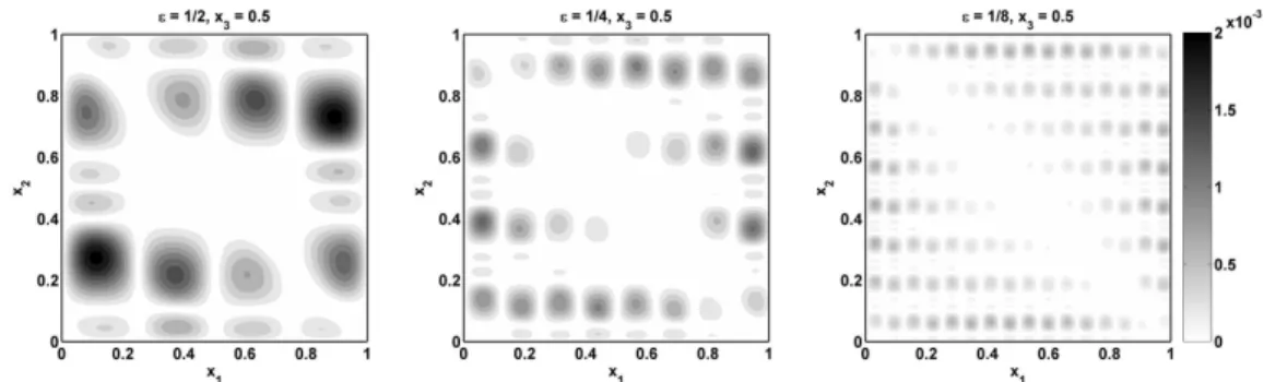
Figure 3: First-order f.a.su(1)(left) and homogenized solutionu0(right).

Figure 4: Absolute differences between the first-order f.a.su(1)and the homogenized solutionu0 forε=1/2,1/4,1/8.

We solve problem (6.6) via separation of variables as in [23], which leads to a Fourier series with orthogonal basis{sin(nπxi)}(n,i)∈N_×{1,2,3}. Then, the solutionu0is

u0(x) = 64 π5

∞

∑

sin(iπx1)sin(jπx2)sin(kπx3)

((2i₋1)2_{+ (2j−1)}2_{+ (2k−1)}2_{) (2i−1)(2j−1)(2k−1)}.

Figures 3 and 4 show the first-order f.a.su(1)and the homogenized solutionu0, and the absolute differences|u(1)₋u0|forε=0.5, 0.25 and 0.125, respectively:

7 CONCLUSIONS

The example presented in this work illustrates the fact that the AHM is an efficient alternative approach to the direct resolution of problems with rapidly oscillating coefficients. Indeed, a di-rect approach via a traditional method, such as the finite difference method used here, would require an extremely fine three-dimensional discretization of the domain in order to capture the rapid variation of the coefficients. This implies a high computational cost and compromises the convergence of the numerical method, which in fact happened when we attempted to solve the original problem of this example by the finite difference method. Thus, AHM provided a useful alternative to obtain an approximate solution of this problem in the form of a formal asymptotic solution, which was proved to be very close to the exact solution. Moreover, from a practical point of view, the problems generated from the application of AHM, that is, the homogenized and local problems, are much easier to solve. In this case, local problems are two-dimensional and their coefficients, although non-constant, they do not oscillate rapidly, which allowed the finite difference method to be successfully applied. Also, as the homogenized problem has con-stant coefficients, it was solved analytically via the Fourier method’s. On the other hand, the search of the exact solution of the original problem would require non-traditional approaches, such as multiscale numerical methods.The example is important for those who will go study the AHM, so know the practical process after applying the method, such: sequence of solve the prob-lems decoupled in the process of homogenization, possible analytical and numerical methods to be used, how to control numerical results for the effective property. This example is a particular case (isotropic property, constant source, homogeneous Dirichlet boundary conditions and con-tinuous coefficients) of much more general and complex problems, but it illustrates essentially the sequence of resolutions to obtain an exact solution approximation, indeed, an approximation ofO₍√_ε).

RESUMO. O m´etodo de homogeneizac¸˜ao assint´otica ´e aplicado para obter a soluc¸˜ao assint´otica formal e uma soluc¸˜ao homogeneizada de um problema de valor de contorno de Dirichlet para uma equac¸˜ao el´ıptica com coeficientes rapidamente oscilantes. A proxi-midade da soluc¸˜ao assint´otica formal e a soluc¸˜ao homogeneizada para a soluc¸˜ao exata ´e provada, a qual fornece a justificativa matem´atica do processo de homogeneizac¸˜ao. A preservac¸˜ao da simetria e definic¸˜ao positiva do coeficiente efetivo no problema ho-mogeneizado ´e tamb´em provada. Um exemplo ´e apresentado para ilustrar os resultados te´oricos.

Palavras-chave: Meio microperi´odico, comportamento efetivo, m´etodo de homogeneizac¸˜ao assint´otica.

REFERENCES

[1] G. Allaire & G. Bal. Homogenization of the criticality spectral equation in neutron transport. Mathematical Modelling and Numerical Analysis,33(4) (1999), 721–746.

[3] M.P. Bendsoe & O. Sigmund. Topology Optimization: Theory, Methods and Applications. Springer-Verlag, New York (2003).

[4] Y. Benveniste. Magnetoelectric effect in fibrous composites with piezoelectric and piezomagnetic phases.Physical Review B,51(1995), 16424–16427.

[5] J. Bravo-Castillero, L.M. Sixto-Camacho, R. Brenner, R. Guinovart-D´ıaz, L.D. P´erez-Fern´andez & F.J. Sabina. Temperature-related effective properties and exact relations for thermo-magneto-electro-elastic fibrous composites.Computers and Mathematics with Applications,69(2015), 980–996.

[6] R.L. Burden & J.D. Faires.Numerical Analysis. Cengage Learning, Canada (2010).

[7] Y. Capdeville, L. Guillot & J.J. Marigo. 1-D non-periodic homogenization for the seismic wave equation.Geophysical Journal International,181(2010), 897–910.

[8] H.J. Choe, K.B. Kong & C.O. Lee. Convergence inLp space for the homogenization problems of elliptic and parabolic equations in the plane.Journal of Mathematical Analysis and Applications,287 (2003), 321–336.

[9] D. Cioranescu & P. Donato.An Introduction to Homogenization. Oxford University Press, New York (1999).

[10] A. Einstein. Eine neue Bestimmung der Molek¨uldimensionen. Annalen der Physik,19(1906), 289– 306.

[11] L.C. Evans.Partial Differential Equations. American Mathematical Society, New York (2010).

[12] A.N. Kolmogorov & S.V. Fomin.Elementos de la Teoria de Funciones y del An´alisis Funcional. Mir, Moscou (1975).

[13] L.D. Kudriavtsev.Curso de An´alisis Matem´atico: Tomo I. Mir, Moscou (1983).

[14] J.C. Maxwell.Treatise on Electricity and Magnetism. Clarendon Press, Oxford (1873).

[15] C.O. Ng. Dispersion in steady and oscillatory flows through a tube with reversible and irreversible wall reactions. Proceedings of the Royal Society of London A: Mathematical, Physical and Engineering Sciences,462(2066) (2006), 481–515.

[16] W.J. Parnell & Q. Grimal. The influence of mesoscale porosity on cortical bone anisotropy. Journal of the Royal Society Interface,6(2009), 97–109.

[17] L.D. P´erezFern´andez & A.T. Beck. Failure detection in umbilical cables via electroactive elements -a m-athem-atic-al homogeniz-ation -appro-ach. International Journal of Modeling and Simulation for the Petroleum Industry,8(2014), 34–39.

[18] L. Rayleigh. On the influence of obstacles arranged in a rectangular order upon the properties of medium.Philosophical Magazine,34(1892), 481–502.

[19] M.H. Sadd.Elasticity: Theory, Applications, and Numerics. Elsevier Academic Press, Oxford (2005).

[21] S. Torquato. Random Heterogeneous Materials: Microstructure and Macroscopic Properties. Springer-Verlag, New York (2002).

[22] S. Torquato. Optimal design of heterogeneous materials. Annual Review of Materials Research,40 (2010), 101–129.