Cultures Results from the Combination of Different
Adaptive Mechanism
Timothe´e Masquelier1,2*, Gustavo Deco1,3
1Unit for Brain and Cognition, Department of Information and Communication Technologies, Universitat Pompeu Fabra, Barcelona, Spain,2Laboratory of Neurobiology of Adaptive Processes (UMR 7102), Centre National de la Recherche Scientifique and University Pierre and Marie Curie, Paris, France,3Institucio´ Catalana de la Recerca i Estudis Avanc¸ats, Universitat Pompeu Fabra, Barcelona, Spain
Abstract
In the brain, synchronization among cells of an assembly is a common phenomenon, and thought to be functionally relevant. Here we used an in vitro experimental model of cell assemblies, cortical cultures, combined with numerical
simulations of a spiking neural network (SNN) to investigate how and why spontaneous synchronization occurs. In order to deal with excitation only, we pharmacologically blocked GABAAergic transmission using bicuculline. Synchronous events in cortical cultures tend to involve almost every cell and to display relatively constant durations. We have thus named these ‘‘network spikes’’ (NS). The inter-NS-intervals (INSIs) proved to be a more interesting phenomenon. In most cortical cultures NSs typically come in series or bursts (‘‘bursts of NSs’’, BNS), with short (,1 s) INSIs and separated by long silent intervals (tens of s), which leads to bimodal INSI distributions. This suggests that a facilitating mechanism is at work, presumably short-term synaptic facilitation, as well as two fatigue mechanisms: one with a short timescale, presumably short-term synaptic depression, and another one with a longer timescale, presumably cellular adaptation. We thus incorporated these three mechanisms into the SNN, which, indeed, produced realistic BNSs. Next, we systematically varied the recurrent excitation for various adaptation timescales. Strong excitability led to frequent, quasi-periodic BNSs (CV,0), and weak excitability led to rare BNSs, approaching a Poisson process (CV,1). Experimental cultures appear to operate within an intermediate weakly-synchronized regime (CV,0.5), with an adaptation timescale in the 2–8 s range, and well described by a Poisson-with-refractory-period model. Taken together, our results demonstrate that the INSI statistics are indeed informative: they allowed us to infer the mechanisms at work, and many parameters that we cannot access experimentally.
Citation:Masquelier T, Deco G (2013) Network Bursting Dynamics in Excitatory Cortical Neuron Cultures Results from the Combination of Different Adaptive Mechanism. PLoS ONE 8(10): e75824. doi:10.1371/journal.pone.0075824
Editor:Michele Giugliano, University of Antwerp, Belgium
ReceivedApril 11, 2013;AcceptedAugust 16, 2013;PublishedOctober 11, 2013
Copyright:ß2013 Masquelier, Deco. This is an open-access article distributed under the terms of the Creative Commons Attribution License, which permits unrestricted use, distribution, and reproduction in any medium, provided the original author and source are credited.
Funding:This work was funded by the European Union Seventh Framework Program (FP7/2007-2013) under grant agreements no. 269459 (Coronet). GD was also supported by the ERC Advanced Grant: DYSTRUCTURE (n. 295129), by the Spanish Research Project SAF2010-16085, and by the CONSOLIDER-INGENIO 2010 Program CSD2007-00012. The funders had no role in study design, data collection and analysis, decision to publish, or preparation of the manuscript.
Competing Interests:The authors have declared that no competing interests exist. * E-mail: [email protected]
Introduction
It is well known that dissociated cultured neuronal networks display spontaneous activity. This activity is not steady but shows instead brief periods (0.1–0.2 s) during which most of the neurons burst – a phenomenon called ‘‘network spikes’’ (NS) – separated by almost silent intervals lasting several seconds [1–11]. Under-standing how and why such synchronization occurs is crucial as synchronization is assumed to play major functional rolesin vivo.
NS’ time courses have been well characterized. For example, it has been shown that typical NS’ rise time is shorter when GABAA
receptors are blocked [4]. Conversely, decay time is shorter when blocking NMDA receptors [11]. Typical time courses also suggest the presence of ‘‘pacemaker’’ neurons and adaptive synapses [9]. In comparison, the laws governing the inter-NS-intervals (INSIs) are much less understood. Certain authors have suggested that the experimentally-observed irregular NSs imply heterogeneities in either neuron properties [12] or synaptic strengths [10]. Other authors have focused on INSI distribution-tails, which has led to controversial results with evidence for both scale-free distributed
INSIs [1] and narrowly-distributed INSIs [5]. However, all authors agree that some fatigue mechanism(s) must be at work to ‘‘quench’’ NS and to enforce a period during which subsequent NSs are much less likely, if not impossible, to occur. Yet the nature and timescales of these mechanisms are still under debate. In the vast majority of simulation studies a single fatigue mechanism was used: either cellular adaptation [2,12], or short-term synaptic depression (STD) [6,9,10,13]. Importantly, these two mechanisms are qualitatively different: adaptation completely prevents subse-quent NSs, while STD only decreases their p [14] bility [14].
In short, we conclude that STD is responsible for quenching NSs, STF for promoting BNSs, and adaptation for interrupting BNSs and for enforcing long inter-BNS-intervals (IBNSIs).
In addition, we systematically varied the SNN excitability for several adaptation timescales. When strong, BNSs are produced almost periodically (CV,0). When weak, BNS generation approaches a Poisson process (CV,1). Experimental values suggest an intermediate semi-regular regime (CV,0.5) with an adaptation timescale in the 2–8 s range. Furthermore, BNS generation, in both experiments and simulations, is reasonably well described by a Poisson-with-refractory-period model, in agreement with previous results [2]. The refractory period lasts about four times as long as the adaptation timescale.
INSIs are thus indeed informative: they allow for both the identification of the mechanisms at work and for the inference of a number of variables which we are unable to access experimentally.
Materials and Methods
Cell preparation
Cortical neurons were obtained from newborn rats (Sprague-Dawley) within 24h after birth using mechanical and enzymatic procedures described in earlier studies [15]. Rats were killed by CO2inhalation according to protocols approved by the National
Institutes of Health. The protocol was approved by the Inspection Committee on the Constitution of the Animal Experimentation at the Technion, approval number IL-099-08-10. The neurons were pre-treated by coating with PEI and then plated onto substrate-integrated multi-electrode arrays, and allowed to develop func-tionally and structurally mature networks over a time period of 2– 3 wk. The number of neurons in a typical network is of the order of 1,300,000, covering an area of 380 mm2. The preparations were bathed in MEM (Sigma-Aldrich), and supplemented with heat-inactivated horse serum (5%), glutamine (0.5 mM), glucose (20 mM), and gentamycin (10mg/ml). They were then maintained at 37uC, 5% CO2-95% air in an incubator and during the
recording phases. An array of 60 Ti/Au/TiN extracellular electrodes, 30mm in diameter and spaced 500mm from each other [MultiChannelSystems (MCS), Reutlingen, Germany], was used (see Fig. 1a). The insulation layer (silicon nitride) was pretreated with polyethyleneimine (Sigma; 0.01% in 0.1 M borate buffer solution).
Electrophysiological recordings
Multi-unit activity (MUA) was recorded using a commercial amplifier (MEA-1060-inv-BC; MCS, Reutlingen, Germany) with frequency limits of 150–3,000 Hz and a gain of X1,024. Data were digitized using a data acquisition board (PD2-MF-64–3M/12H; UEI, Walpole, MA). Each channel was sampled at a frequency of
16 k samples/s. Data processing was performed using a Simulink-(The Mathworks, Natick, MA, USA) based xPC target application (see ref. [16] for details). We added 6mM bicuculline–methiodide
to the bathing solution, and given that the dissociation constant is around 5mM [17] this was assumed to block most of the inhibitory
transmission.We used a total of seven recordings, each one corresponding to a different culture: one 2h-recording, four 1h-recordings, two 1/2h- recordings. Ages ranged from 14 to 35 days in vitro (DIV). Spike sorting was not attempted.
Neuron model
The network consists inNE~800excitatory neurons.
Connec-tivity is full. We used conductance-based leaky integrate and fire (LIF) neurons. Their membrane potentialVobeys the following Langevin equation:
CmdV
dt~{gmðV{VLÞ{IsynzIAHPzs
ffiffiffiffiffiffiffiffiffiffiffiffiffiffiffi 2gmCm p
j, ð1Þ
Where gm~1=Rm is the membrane leak conductance, Cm its
capacitance,VLis the resting potential,Isynis the synaptic current (described in the next section),IAHPis the After-HyperPolarization adapting current (described in the Adaptation section), j is a Gaussian white noise (withSjð Þt T~0andSx tð Þx sð ÞT~dðt{sÞ), and s is the standard deviation of the resulting noise in the membrane potential. The membrane time constant is defined by
tm~Cm=gm. When the membrane potential reaches the threshold Vthr the neuron generates a spike, which is then transmitted to other neurons. Next, the membrane potential is instantaneously reset toVreset and is maintained there for a refractory timetref, during which the neuron is unable to produce further spikes (see Table 1 for parameter values).
Synapse model
Spikes arriving at a given neural synapse induce post-synaptic excitatory potentials (EPSP), essentially given by a low-pass filtering formed through the synaptic receptors. In our case, the total synaptic current is given by the sum of glutamatergic AMPA (IAMPA) and NMDA (INMDA) recurrent excitatory currents:
Isyn~IAMPAzINMDA, ð2Þ
where:
IAMPAð Þt~gAMPAðV tð Þ{VEÞPNE j~1
wjsAMPA
j ð Þt , ð3Þ
a
0 40
0 50 100
Spike/s/electrode
b
t (s)
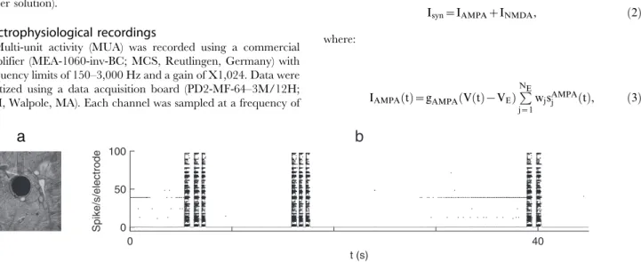
Figure 1. Spontaneous activity in neuronal cultures.(a) Cortical network on substrate-embedded multielectrode array. The dark circle is a
30-mm-diameter electrode. Figure is modified from ref. [4]. (b) Raster plot showing the spikes recorded at each of the 60 electrodes (black dots) as a
INMDAð Þt ~gNMDAðV tð Þ{VEÞ 1zce{bV tð Þ
XNE
j~1
wjsNMDAj ð Þt , ð4Þ
HeregAMPA andgNMDA are the synaptic conductances, andVE
the excitatory reversal potentials. The dimensionless parameters
wjof the connections are the synaptic weights (subject to short-term plasticity, see Eq. 11). The NMDA currents are voltage-dependent and they are modulated by intracellular magnesium concentration c. The gating variables si
jð Þt are the fractions of
open channels of neurons, and are given by:
dsAMPA j ð Þt
dt ~{
sAMPA j ð Þt
tAMPA z X
k
dt{tkj{D, ð5Þ
dsNMDAj ð Þt
dt ~{
sNMDAj ð Þt
tNMDA,decay
zaxNMDAj ð Þt 1{sNMDAj ð Þt
, ð6Þ
dxNMDAj ð Þt
dt ~{
xNMDA j ð Þt
tNMDA,rise zX
k
dt{tkj{D ð7Þ
HerexNMDA
j is an auxiliary gating variable for NMDA, andais a
multiplicative constant. The sums over the indexk represent all the spikes emitted by the presynaptic neuron j (at times tk
j). In
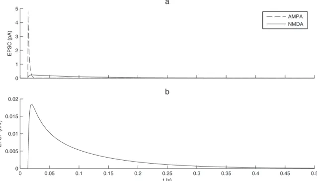
Equations (5-7),tNMDA,riseandtNMDA,decayare the rise and decay times for the NMDA synapses, andtAMPA the decay times for AMPA synapses. The AMPA synapse rise time is neglected because it is very short (,1 ms).Dis a homogeneous conduction delay. The values of the constant parameters and default values of the free parameters used in the simulations are displayed in Table 1. Figure 2 illustrates the different time-courses of NMDA and AMPA synaptic currents and the resulting EPSP.
Adaptation model
A spike-frequency adapting mechanism is taken into account. It is implemented in the network by including an additional leakage after-hyperpolarization currentIAHPinto the dynamical equation
of the membrane potential of each neuron, given by the following equation:
IAHPð Þt~{gaðV tð Þ{VaÞ ð8Þ
whereVais the reversal potential andgað Þt the effective additional
leak conductance.
gað Þt is initially set to 0. Between spikes, it is modeled as a leaky
integrator with a decay time constantta:
tadga
dt ~{ga: ð9Þ
IfV tð Þ~Vthr, a spike is emitted and
V?Vthr
ga?gaza
ð10Þ
This adapting current may correspond to slow calcium- and sodium-activated potassium currents, but also to other fatigue mechanisms. ta is the apparent recovery timescale of all these combined mechanisms, which, as we will see, may vary from one culture to another.
Short-term plasticity model
All synapses are modulated by short-term plasticity (STP). The phenomenological model proposed in ref. [18] was used. It is based on the concept of the utilization of synaptic efficacy u, of which only a fraction x is available:
0vxjv1 Uvujv1 wj~uj:xj:W0 8
> <
> :
: ð11Þ
They obey a differential equation:
dxj dt~
1{xj tD {uj
:xj:X
k
dt{tkj{D ðDepressionÞ
duj dt~
U{uj
tF zU: 1{uj
:X
k
d t{tk j{D
Facilitation
ð Þ
8 > > > <
> > > :
:ð12Þ
In other words, for each presynaptic spike:
uis increased byU 1ð {uÞ xis multiplied byð1{uÞ.
Between presynaptic spikes:
xrelaxes towards 1 with time constanttD urelaxes towardsUwith time constanttF
Numerical parameters
Table 1 gathers the neuronal parameters taken from ref. [19]. An additional parameterdallows us to modify the ratio between AMPA and NMDA currents [20]:
gNMDA?ð1{dÞgNMDA gAMPA?ð1z10dÞgAMPA
The factor 10 results from the fact that near the firing threshold the ratio of NMDA to AMPA components becomes 10 to 1 in terms of charge entry [19]. We usedd~0:08, as in ref. [21].
Table 1.Neuronal and synaptic parameters.
Excitatory Neurons Synapses
NE 800 neurons VE 0 mV
Cm 0.5 nF VI 270 mV
gm 25 nS tAMPA 2 ms
VL 270 mV tNMDA,rise 2 ms
Vthr 250 mV tNMDA,decay 100 ms
Vreset 255 mV tGABA 10 ms
tref 2 ms a 0.5 kHz
gAMPA,rec 0.104 nS b 0.062
gNMDA,rec 0.327 nS c 0.28
gGABA 1.250 nS
For the Gaussian white noise, we useds~6:5mV.
For conduction delays (homogeneous), we usedD~3ms(which
is in the biological range, see ref. [22]).
For STP, we used tD~800ms (in the biological range, see [9,13,14,18,23]), tF~1600ms, and U~0:025 (both in the
biological range, see ref. [18]). As we will see in the Result section, the mechanism that we propose for BNS requires that
tDvtF, as found in ref. [18]. We note, however, that other groups have reportedtDwtF (see ref.[24] for a review).
For adaptation, we used (unless said otherwise): ta~4s,
a~0:145nS,Va~{80mV.
Simulations
We developed custom python code for the Brian clock-based simulator [25]. The differential equations were integrated numerically (Euler method) using a 25ms-time step. The code
has been made available on ModelDB (http://senselab.med.yale. edu/modeldb/ShowModel.asp?model = 150437).
Detecting NS
In both the cultures and the model, NSs have an all-or-none nature and are thus easy to detect. Therefore, we just counted the spikes recorded at all electrodes in 50ms-time bins and used a threshold equal toJof the maximum spike count recorded over the session. We verified that the results were not very sensitive to this threshold, nor to the bin duration.
Results
Spontaneous NS with bimodal INSI distributions
In all our cultures, neurons are spontaneously active (Fig. 1b), and spontaneously synchronize every 1–50 s. These synchronous events typically involve the whole network [4], hence the denomination ‘‘network spikes’’. While the firing rates during such NSs can reach 100 spikes/electrode/s or more, it is typically
of ,1spike/electrode/s between NSs or less (Fig 1b, gray line). NSs are thus easy to detect, for example using a simple rate threshold (see Materials and Methods). The results are not very sensitive to the threshold nor to the time bin size.
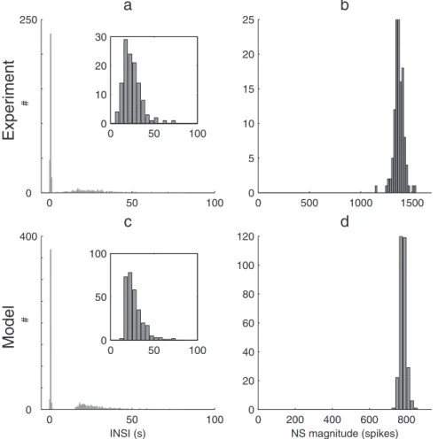
In most cultures, NSs are not ‘‘isolated’’, but come in series (‘‘burst of NSs’’, BNS) with short INSIs (,1 s or less), while the intervals between BNSs are substantially longer (tens of s), leading to bimodal INSI distributions (Fig. 3a). Importantly, these BNSs are also commonly seen without blocking the GABAAreceptors
[5]. The inset zooms in on the long INSIs (.6 s). Notably, their distribution is slightly positively skewed, with a somewhat long tail (we will come back to this point in the Working point identification section).
Conversely, the NS magnitudes, expressed here in total number of spikes emitted, appear to be normally distributed (Fig. 3b), with a small standard deviation (lower than 4% of the mean). Note, however, that we only included the first NS of each series; subsequent ones tend to be weaker due to fatigue mechanisms. Durations and maximum firing rates are also narrowly distributed (data not shown). This confirms the all-or-none nature of NSs previously reported in similar preparations, especially when using bicuculline [4]. Magnitude statistics are thus not very informative here.
Our goal was now to come up with a minimal spiking neural network (SNN) model. It had to be as simple as possible, and yet able to produce all-or-none NSs with bimodal INSI distributions (Fig. 3c and d). What were the key ‘‘ingredients’’ needed? As mentioned above, GABAA receptors were blocked in the
experimental recordings. Thus, inhibitory neurons were not expected to impact on the dynamics and for the sake of simplicity we thus ignored them in our model.
Implications for the mechanisms at work
To trigger an NS, two things are needed: random fluctuations and positive feedback [12]. In our model, the random fluctuations
0 1 2 3 4 5
a
EPSC (pA)
AMPA NMDA
0 0.05 0.1 0.15 0.2 0.25 0.3 0.35 0.4 0.45 0.5 0
0.005 0.01 0.015 0.02
b
EPSP (mV)
t (s)
Figure 2. Excitatory postsynaptic currents and potentials.(a) NMDA and AMPA current dynamics after the arrival of one presynaptic spike.
are caused by the Gaussian white noise (j in Eq. (1)). The recurrent excitatory connections, whose strength can be adjusted (W0 in Eq. (11)), provide the positive feedback, causing an exponential recruitment of cell activity in the early phase of each NS [12], as observed experimentally [4].
Next, what are the mechanisms responsible for quenching the NS? The candidate restoring forces are: the recruitment of the inhibitory network (which can be discarded when blocking GABAAreceptors like here), cellular refractoriness and adaptation,
and short-term synaptic depression (STD). The long (,20–30 s), semi-regular (CV,0.5) inter-BNS-intervals (IBNSI, Fig. 3a inset) imply that at least one of these mechanisms has a long timescale (,2–8 s, see Working point identification section). This is most probably adaptation or STD, since cellular refractoriness is typically in the millisecond range.
Besides, as said above, INSI distributions are often bimodal. In other words, the probability of getting an NS is higher if there was another one in a recent past (,1 s), even if activity has returned to baseline. This suggests that a facilitating mechanism is at work, most probably short-term synaptic facilitation (STF). Alternatively, this could be due to waves of activity reverberating along the network border, where connectivity is denser, and returning to the point where the NS started with sufficient delay to find neurons ready to fire again and ignite another NS [23]. This possibility,
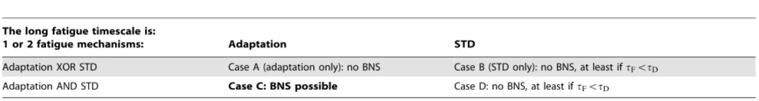
demonstrated in large-scale simulations (10,000–50,000 neurons) [23], is not considered further in this paper. Hence we assume that STF is at work, with a time constanttFin the 1–3 s range (which is in broad agreement with the experimental estimation of 179761247 ms [18]), and that there is at least one fatigue mechanism with a long timescale (,2–8 s). This left us with four possible scenarios (Table 2): the long fatigue timescale could correspond to STD, or to cellular adaptation; and there could be two or just one fatigue mechanism. To rule these four scenarios in or out we performed exhaustive searches on the numerical parameters (Table 2).
Using strong adaptation (highain Eq. 10) we observed that it is possible to quench an NS without STD (case A in Table 2). But each NS is then followed by a period in which the network is completely silent (data not shown). Thus facilitation, which modulates input spike effect, did not help in triggering subsequent NSs, and the network only produced isolated NSs. In other words, we confirmed the results of ref. [14]: adaptation enforces a hard refractory period, which prevents BNSs, while STD only decreases NS probability, which can be compensated by STF. Case A was thus ruled out.
Using only STD with a long timescaletDwtF(case B), again we were only able to produce isolated NSs. Indeed, iftDwtF, then the net effect of short-term plasticity (STP) shortly after an NS is
0 50 100
0 250
a
Experiment
#
0 50 100
0 10 20 30
0 500 1000 1500
0 5 10 15 20 25
b
0 50 100
0 400
c
INSI (s)
Model
#
0 50 100
0 50 100
0 200 400 600 800
0 20 40 60 80 100 120
d
NS magnitude (spikes)
Figure 3. INSI and NS magnitude histograms.(a) Experimental INSI distribution in one representative culture, using 500 ms time bins. The
distribution is bimodal, with either very short INSIs (,1.5 s) or much longer ones (.6 s).The inset zooms on the long INSIs (.6 s) and uses a larger time bin (5 s). Notice the (somewhat) long tail: the distribution is positively skewed. (b) Conversely, the experimental NS magnitude distribution is unimodal and quite narrow (only the first NS of each BNS is taken into account). (c and d) Same histograms for the model, withW0~8:75andtaw4s
(Note that we fitted the NS timescales, but not their magnitudes. Indeed, we do not know how many neurons each electrode picks on average; therefore we cannot estimate the true average number of spikes per second per neuron).
depressing and does not promote subsequent NSs. Obviously, adding adaptation here (case D) did not help us in getting BNSs. We verified that it is possible to produce BNSs usingtFwtD,2– 8 s. However, not only were these time constants not very realistic, but the intra-BNS INSIs were several seconds long, in contradic-tion with experimental observacontradic-tion (1 s or less, see Fig. 3a). Accordingly, both cases B and D were largely ruled out.
That left us with case C. STD is at work with a short timescale
tDvtF (respectively 0.8 and 1.6 s in the baseline simulation, see Fig. 4). Hence the net result of STP shortly after an NS is facilitative (Fig. 4b), promoting BNSs. Long timescale (weak) adaptation is responsible for both interrupting the series, and for enforcing long IBNSIs (Fig. 4c). However, the main restoring force quenching each NS is STD, in line with experimentation [26] and seminal modeling work [13].
Note that this reasoning would not have been possible without blocking GABAA receptors, because inhibition would have
provided a third restoring force, of which the timescale would be unclear [23]. But of course it seems reasonable to assume that the mechanisms we have identified, namely STP and cellular
adaptation, with tDvtFvta, are also at work when GABAA receptors are unblocked – although obviously the resulting dynamics changes.
Fatigue timescales’ separation
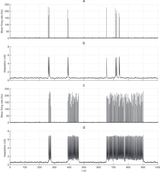
As we have explained above, we suggest that STP with its time constantstDvtFshapes short intra-BNS INSIs, while adaptation, with a longer time constantta, shapes the long IBNSIs. To what extent didtaneed to be greater thantDandtFin order to obtain realistic BNSs? We kepttD= 0.8 s andtF= 1.6 s, and performed an exhaustive search onta, keepingta:aconstant (to maintain the global level of adaption, see Eq. 9–10). It turned out that a qualitative change of regime occurs between ta= 1.2 s and
ta= 1.6 s (Fig. 5).
For ta= 1.6 s (as in Fig. 4), adaptation conductance can accumulate across intra-BNS NSs until it is high enough to prevent subsequent NSs and the series terminates (Fig. 5a and b). In this regime, BNS initiation is stochastic. What happens next, however (exponential recruitment, STD-induced activity decay, STF-induced subsequent NSs, adaptation-induced series
Table 2.Ruling in and ruling out fatigue mechanisms.
The long fatigue timescale is:
1 or 2 fatigue mechanisms: Adaptation STD
Adaptation XOR STD Case A (adaptation only): no BNS Case B (STD only): no BNS, at least iftFvtD
Adaptation AND STD Case C: BNS possible Case D: no BNS, at least iftFvtD doi:10.1371/journal.pone.0075824.t002
0 200 400
a
Mean firing rate (Hz)
0 0.5 1
b
Short−term plasticity
x u u.x
80 85 90 95 100 105 110 115 120 125 130
0 2 4 6
c
Adaptation (nS)
t (s)
Figure 4. Model neurodynamics.(a) Raster plot showing the spikes of 60 neurons (black dots) as a function of time. The gray line shows the mean
population firing rate (b) STP variables (population-averaged) as a function of time. Notice that, sincetD~0:8svtF~1:6s, depression X recovers faster than facilitation u after an NS. Thus the net STP modulation u.X shortly after an NS is facilitating, promoting subsequent NSs. (c) Adaptation leak conductance ga(population-averaged) as a function of time. It accumulates after each NS. When too strong, the NS series is interrupted, and followed
by a long silent interval.
termination), is much more deterministic, yet not fully so. A similar regime has been identified in SNNs with adaptation but without STP, and thus without resulting in BNSs [27].
Forta= 1.2 s, the adaptation conductance cannot accumulate across intra-BNS NSs. Thus, it will not systematically terminate the BNS. Instead, BNS termination is stochastic, which can lead to very long BNSs (Fig. 5c and d). Such long BNSs have not been observed in our cultures.
Hence, to get a clear separation of STP and adaptation timescales, a necessity to get realistic BNSs,taneeds to be greater
than 1.2 s. This is consistent with the experimental range estimated in the next section: 2–8 s.
Working point identification
In the following section, we will focus on long IBNSIs (.6 s, see Fig. 3a and 3c insets). As explained above, two things are needed to trigger an NS: a random fluctuation of a certain magnitude, and a recurrent excitation that provides positive feedback. We systematically varied excitability in the model (i.e. the recurrent excitatory weightW0 in Eq. 11), keeping the noise parameters
constant. As expected, the BNS frequency (respectively the mean
0 50 100 150 200 250
Mean firing rate (Hz)
a
0 2 4 6 8
b
Adaptation (nS)
0 50 100 150 200 250
Mean firing rate (Hz)
c
0 100 200 300 400 500 600 700 800 900 1000 0
2 4 6 8
d
Adaptation (nS)
t (s)
Figure 5. Fatigue timescales’separation. For panels (a–b)ta= 1.6 s, while for panels (c–d)ta= 1.2 s. In all cases,tD= 0.8 s,tF= 1.6 s, and
W0= 8.6 (a) Mean population firing rate as a function of time. (b) Adaptation leak conductance ga(population-averaged) as a function of time. Inside a
BNS, it tends to accumulate across successive NSs, until it is high enough to prevent subsequent NSs. Thus BNS termination is almost deterministic, while BNS initiation is stochastic. (c) Mean population firing rate as a function of time. (d) Adaptation leak conductance ga(population-averaged) as a
function of time. It cannot accumulate across successive NSs. Thus both BNS initiation and termination are stochastic. This can lead to hundreds of ms long BNSs, which is not realistic.
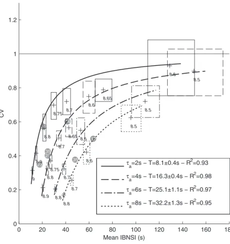
IBNSI) increased (resp. decreased) with W0 (Fig. 6), because smaller fluctuations become sufficient to trigger NSs.
In addition, the shape of the IBNSI distribution changes. In the case of large excitability as soon as the adaptation-induced refractory period is over (say, after a fewtas), an NS is rapidly produced, because the required weak fluctuation appears quickly (see also Fig. 7). Consequently, the IBNSI are regular; that is, their coefficient of variation (CV) is low (Fig. 6). Conversely, with low excitability, the required strong fluctuation may take longer to appear, leading to a positively skewed IBNSI distribution.
In the limit caseW0?0, neurons are independent. They spike only due to the independent white noise they receive (jin Eq. 1), with very long mean inter spike interval (,2 s with our parameters). At such low rates spike generation approaches a Poisson process (individual CV ,1). Thus, spike coincidences between neurons, which cause the required fluctuations, also follow a Poisson process. As a result, the IBNSI CV approaches 1, while NS becomes extremely rare (Fig. 6). It is worth noting that even whenW0~0, one is guaranteed to see an NS if one waits long enough, as at some point the independent neurons will fire synchronously. In practice, however, and with reasonable time bins and thresholds for NS detection, the expected waiting time would be astronomical.
In addition, we also varied the adaptation time constant ta
(Fig. 6), from 2 to 8 s, keepingta:aconstant (to maintain the global level of adaption). This shifted the curve of all possible (CV, Mean INSI) values either up or down.
We then wanted to test how well BNS generation in the model may be described by a Poisson point process with refractory period T[28]. In such processes, theCVis linked to the mean intervalm
by CV~(m{T)=m. We thus fitted one model of this kind for eachtavalue (Fig. 6), adjustingT. We used the non-linear least square method and we assigned a weight to each data point that was inversely proportional to its error box area. The legend shows estimated refractory periodsT, which turned out to be around 4ta. This confirms that the cause here of the refractory period is adaptation, as opposed to STD. Overall, the fittings were good (R2$0.93), indicating that the Poisson process with refractory period sis a reasonable model for BNSs. This was also the conclusion of a previous simulation study [2], which did not, however, include STP, and thus had only isolated NSs. The goodness of fit also confirms that adaptation has the capacity to enforce a hard refractory period [14].
Finally, we placed our seven experimental data points, corresponding to the different cultures on the (Mean IBNSI, CV) plane (Fig. 6, gray circles). This allowed us to determine for
0 20 40 60 80 100 120 140 160 180
0 0.2 0.4 0.6 0.8 1 1.2
24
25
23
14
35 35
17
8.8 8.7
8.6
8.5
8.8 8.7
8.6
8.5
8.9 8.8
8.75 8.7
8.65 8.6
8.5
9 8.9
8.8 8.75 8.7
8.65
8.6
CV
Mean IBNSI (s)
τ
a=2s − T=8.1±0.4s − R 2
=0.93
τ
a=4s − T=16.3±0.4s − R 2
=0.98
τ
a=6s − T=25.1±1.1s − R 2
=0.97
τ
a=8s − T=32.2±1.3s − R 2
=0.95
Figure 6. Working point.Each curve corresponds to all the possible (Mean IBNSI, CV) points that the model can reach by varying the recurrent
excitatory weight W0(see values in italic), keepingtaconstant. Simulations stopped when 300 BNSs were recorded (with an additional 5h limit). Cases
with less than 100 BNSs were discarded. The boxes represent 95% confidence intervals (estimated with bootstrapping), for both CV and mean IBNSI. We fitted a Poisson-with-refractory-period model CV = (mean-T)/mean for eachtavalue. The legend shows estimated refractory periods T, with 95%
confidence intervals, and the coefficients of determination R2. Gray circles represent the experimental cultures, and the numbers inside are the
corresponding days in vitro (DIV), which did not correlate with the mean INSIs, or the CV. The horizontal gray line materializes the asymptotic limit CV = 1.
each culture, and without ambiguity, the apparent timescale of adaptation ta (given by the unique curve passing through the experimental point), which turned out to be in the 2–8 s range, and then the strength of recurrent excitationW0needed to reach that particular point on the curve.This strength could be mapped to the density of excitatory synapses. Remarkably, this inference was possible using the IBNSI statistics only. All cultures appeared to operate in an intermediate, weakly-synchronized regime with semi-regular BNS (CV,0.5).
The Kolmogorov-Smirnov statistical test used in ref. [28] failed to provide evidence for power-law distributed, rather than exponentially-distributed IBNSIs, in both experimental and simulated data. This is again consistent with the Poisson point process with refractory period, which leads to interval distributions with exponentially decaying tails.
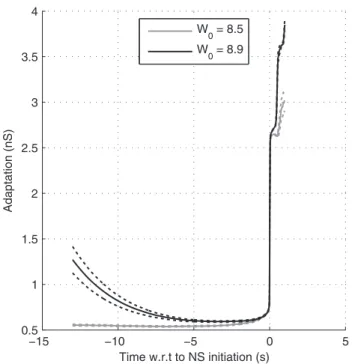
We also plotted the NS-triggered average of the adaptation leak conductance ga, in case of strong (respectively weak) recurrent
excitation producing regular (resp. irregular) NSs (Fig. 7). As was expected in the regular case, a relaxed adaptation conductance is a necessary and sufficient condition for NS generation (black curve). In the irregular case, it was only a necessary condition. A significant fluctuation also needs to appear and this may take some time During this waiting period the adaptation conductance was typically low (gray curve).
Discussion
Time series of network synchronization events (NSs) demon-strate complex statistics, both in vivoand in vitro. Current models fall short of explaining these statistics. Here, we have shown that the incorporation of three adaptive processes (short-term synaptic facilitation, fast and slow fatigue) is sufficient to reconstruct the experimentally- observed complex statistics. Our theoretical framework was adjusted and validated by fitting to a data set we
had obtained from in vitro large-scale networks of excitatory cortical neurons.
INSI statistics appear to have been somewhat overlooked by many of the community. Most researchers focus on characterizing and explaining NSs’ magnitudes and durations. For example, in a number of preparations, these two variables have been shown to follow power-law (scale-free) distributions [7,8], much like the so-called ‘‘neuronal avalanches’’ in organotypic cultures and acute cortical slices [29]. These power-laws, which seem to hold only with inhibition [11,29,30] have been interpreted as a signature of self-organized criticality (but see ref. [31,32]), which is theoretically appealing [29,30,33,34].
In our experiments inhibition was blocked, and therefore NS magnitudes were narrowly distributed. However, INSI statistics turned out to be more interesting. They enabled us, firstly, to infer the mechanisms at work, and secondly to estimate their timescales. More specifically, bimodal INSI distributions suggest that both STP and adaptation are at work, withtDvtFvta. In short, STD is responsible for quenching the NS, STF for promoting BNSs, and adaptation for interrupting the BNSs and enforcing long IBNSIs. The long modes of the INSI distributions unambiguously determine variables which we cannot access experimentally, namely ta and the excitability. In turn, the variables determine the system’s working point. With strong excitability, IBNSI are short and regular (low CV), while with weak excitability NS generation approaches a Poisson process with extremely long irregular IBNSIs (CV,1). It seems that experimental cultures operate in an intermediate mode, producing semi-regular IBNSIs (CV,0.5) with a slightly positively-skewed distribution. A Poisson-with-refractory-period model fits well with both simulated and experimental IBNSI.
Importantly, we used a simple full non-plastic connectivity (although random sparse ones gave similar results, data not shown). It is likely that some modularity is needed to obtain more graded, possibly power-law-distributed, NS magnitudes [34]. Spike timing-dependent plasticity may also help [34]. However, evidence for such power-laws in dissociated cultured neuronal networks remains rare [7,8]. In our experiments we observed stereotyped almost all-or-none NSs, in line with previous reports [4]. Power-law-distributed sizes and durations are more estab-lished in organotypic cultures and acute cortical slices [29,35], possibly because they have the required connectivity.
Remarkably, a full connectivity with homogeneous synaptic weights turned out to be sufficient to capture the experimentally-observed INSI statistics. Our neurons were indistinguishable, and yet we observed non-periodic NSs. This could be seen as incongruent with simulations that have shown that non-homoge-neous cell properties [12] or synaptic weights [9] are required for non-periodic synchronization. We admit, however, to injecting a fair amount of independent white noise current to each neuron. This noise may be playing a similar role as non-homogeneities.
However, a full connectivity with homogeneous weights is clearly a limitation. Among other things, we cannot capture the fact that some neurons are much more active than others, and that an upcoming NS can be reliably predicted based on the activity of a few ‘‘privileged’’ neurons as early as 100ms before the NS peak [4].
NS in neuron cultures is a robust and well-documented phenomenon [1–11]. These in vitro preparations offer an ideal framework to combine experimental work with simulations. Experimental conditions can be much more carefully controlled than in mostin vivoexperiments. In particular, the external inputs may be fully controlled or canceled (as in our experiments), and pharmacological manipulations are also possible. However, it is worth mentioning that NS-like synchronous events have been
−15 −10 −5 0 5
0.5 1 1.5 2 2.5 3 3.5 4
Time w.r.t to NS initiation (s)
Adaptation (nS)
W
0 = 8.5
W
0 = 8.9
Figure 7. Adaptation in regular vs. irregular mode. Here we
plotted the population-averaged adaptation leak conductance ga
preceding the BNSs, averaged across 100 BNSs, with W0= 8.5 and 8.9
(andta= 4 s). Dotted lines show 95% confidence interval for the mean.
observedin vivoas well: in the cortex [36–38], the hippocampus [39], and in LGN [40].
Synchronization is thought to play major functional roles in the brain. Individual neurons are sensitive to synchronous inputs [41,42] and these are favored by synaptic plasticity mechanisms [43]. At the level of cell assembly, synchrony is thought to enable feature binding [44], communication through coherence [20,45], and phase-of-firing coding [46,47]. Understanding how and why synchronization occurs is thus of crucial importance, and as we have argued here,in vitroneuronal cultures might be useful as an experimental model for generic cell assembly. One must, however, keep in mind the obvious constraints on extrapolations fromin vitro to in vivo conditions, in particular because the networks are no longer isolated (for review, see ref. [15,48]).
Acknowledgments
We are greatly indebted to Shimon Marom and Netta Haroush, from Technion at the Israel Institute of Technology, who provided us with the experimental data. We would also like to thank Dan Goodman and Romain Brette for having developped the efficient and user-friendly Brian simulator [25], as also for their excellent support, Mikail Rubinov for sharing his implementation of the Kolmogorov-Smirnov statistical test for power-law distributions with us, Tom Morse and ModelDB [49] for distributing our code, and finally Michael Kolkman (http://helice.nl) for his excellent language polishing work.
Author Contributions
Conceived and designed the experiments: TM GD. Performed the experiments: TM. Analyzed the data: TM. Wrote the paper: TM.
References
1. Segev R, Benveniste M, Hulata E, Cohen N, Palevski A, et al. (2002) Long term behavior of lithographically prepared in vitro neuronal networks. Phys Rev Lett 88: 118102.
2. Giugliano M, Darbon P, Arsiero M, Lu¨scher H-R, Streit J (2004) Single-neuron discharge properties and network activity in dissociated cultures of neocortex. Journal of neurophysiology 92: 977–996. Available: http://dx.doi.org/10.1152/ jn.00067.2004. Accessed 24 August 2013.
3. Van Pelt J, Vajda I, Wolters PS, Corner MA, Ramakers GJA (2005) Dynamics and plasticity in developing neuronal networks in vitro. Progress in brain research 147: 173–188. Available: http://dx.doi.org/10.1016/S0079-6123(04)47013-7. Accessed 7 August 2013.
4. Eytan D, Marom S (2006) Dynamics and effective topology underlying synchronization in networks of cortical neurons. The Journal of neuroscience: the official journal of the Society for Neuroscience 26: 8465–8476. Available: http://dx.doi.org/10.1523/JNEUROSCI.1627-06.2006. Accessed 9 August 2013.
5. Wagenaar DA, Pine J, Potter SM (2006) An extremely rich repertoire of bursting patterns during the development of cortical cultures. BMC neuroscience 7: 11. Available: http://dx.doi.org/10.1186/1471-2202-7-11. Accessed 13 August 2013.
6. DeMarse TB, Principe JC (2006) Modeling of Synchronized Burst in Dissociated Cortical Tissue: An Exploration of Parameter Space. The 2006 IEEE International Joint Conference on Neural Network Proceedings. IEEE. p. 581–586. Available: http://ieeexplore.ieee.org/lpdocs/epic03/wrapper. htm?arnumber = 1716145. Accessed 24 August 2013.
7. Pasquale V, Massobrio P, Bologna LL, Chiappalone M, Martinoia S (2008) Self-organization and neuronal avalanches in networks of dissociated cortical neurons. Neuroscience 153: 1354–1369. Available: http://dx.doi.org/10.1016/ j.neuroscience.2008.03.050. Accessed 15 August 2013.
8. Tetzlaff C, Okujeni S, Egert U, Wo¨rgo¨tter F, Butz M (2010) Self-organized criticality in developing neuronal networks. PLoS computational biology 6: e1001013. Available: http://dx.plos.org/10.1371/journal.pcbi.1001013. Ac-cessed 14 August 2013.
9. Gritsun TA, Le Feber J, Stegenga J, Rutten WLC (2010) Network bursts in cortical cultures are best simulated using pacemaker neurons and adaptive synapses. Biological cybernetics 102: 293–310. Available: http://dx.doi.org/10. 1007/s00422-010-0366-x. Accessed 16 August 2013.
10. Gritsun T, le Feber J, Stegenga J, Rutten WLC (2011) Experimental analysis and computational modeling of interburst intervals in spontaneous activity of cortical neuronal culture. Biological cybernetics 105: 197–210. Available: http://dx.doi. org/10.1007/s00422-011-0457-3. Accessed 16 August 2013.
11. Baltz T, Herzog A, Voigt T (2011) Slow oscillating population activity in developing cortical networks: models and experimental results. Journal of neurophysiology 106: 1500–1514. Available: http://dx.doi.org/10.1152/jn. 00889.2010. Accessed 24 August 2013.
12. Thivierge J-P, Cisek P (2008) Nonperiodic synchronization in heterogeneous networks of spiking neurons. The Journal of neuroscience: the official journal of the Society for Neuroscience 28: 7968–7978. Available: http://dx.doi.org/10. 1523/JNEUROSCI.0870-08.2008. Accessed 24 August 2013.
13. Tsodyks M, Uziel A, Markram H (2000) Synchrony generation in recurrent networks with frequency-dependent synapses. J Neurosci 20: RC50. 14. Wiedemann UA, Lu¨thi A (2003) Timing of network synchronization by
refractory mechanisms. Journal of neurophysiology 90: 3902–3911. Available: http://www.ncbi.nlm.nih.gov/pubmed/12930814. Accessed 24 August 2013. 15. Marom S, Shahaf G (2002) Development, learning and memory in large
random networks of cortical neurons: lessons beyond anatomy. Q Rev Biophys 35: 63–87.
16. Zrenner C, Eytan D, Wallach A, Thier P, Marom S (2010) A generic framework for real-time multi-channel neuronal signal analysis, telemetry control, and sub-millisecond latency feedback generation. Frontiers in neuroscience 4: 173. Available: http://dx.doi.org/10.3389/fnins.2010.00173. Accessed 24 August 2013.
17. Frere RC, Macdonald RL, Young AB (1982) GABA binding and bicuculline in spinal cord and cortical membranes from adult rat and from mouse neurons in cell culture. Brain research 244: 145–153. Available: http://www.ncbi.nlm.nih. gov/pubmed/6288176. Accessed 24 August 2013.
18. Markram H, Wang Y, Tsodyks M (1998) Differential signaling via the same axon of neocortical pyramidal neurons. Proc Natl Acad Sci U S A 95: 5323– 5328.
19. Brunel N, Wang XJ (2001) Effects of neuromodulation in a cortical network model of object working memory dominated by recurrent inhibition. Journal of computational neuroscience 11: 63–85. Available: http://dx.doi.org/10.1023/ A:1011204814320. Accessed 24 August 2013.
20. Buehlmann A, Deco G (2008) The neuronal basis of attention: rate versus synchronization modulation. The Journal of neuroscience: the official journal of the Society for Neuroscience 28: 7679–7686. Available: http://dx.doi.org/10. 1523/JNEUROSCI.5640-07.2008. Accessed 22 August 2013.
21. Albantakis L, Deco G (2011) Changes of mind in an attractor network of decision-making. PLoS computational biology 7: e1002086. Available: http:// dx.doi.org/10.1371/journal.pcbi.1002086. Accessed 24 August 2013. 22. Nakanishi K, Kukita F (1998) Functional synapses in synchronized bursting of
neocortical neurons in culture. Brain Res 795: 137–146.
23. Gritsun TA, le Feber J, Rutten WLC (2012) Growth dynamics explain the development of spatiotemporal burst activity of young cultured neuronal networks in detail. PloS one 7: e43352. Available: http://dx.plos.org/10.1371/ journal.pone.0043352. Accessed 26 March 2013.
24. Zucker RS, Regehr WG (2002) Short-term synaptic plasticity. Annual review of physiology 64: 355–405. Available: http://www.ncbi.nlm.nih.gov/pubmed/ 11826273. Accessed 24 May 2013.
25. Goodman D, Brette R (2008) Brian: a simulator for spiking neural networks in python. Frontiers in neuroinformatics 2: 5. Available: http://dx.doi.org/10. 3389/neuro.11.005.2008. Accessed 14 August 2013.
26. Eytan D, Brenner N, Marom S (2003) Selective adaptation in networks of cortical neurons. J Neurosci 23: 9349–9356.
27. Gigante G, Mattia M, Giudice P Del (2007) Diverse population-bursting modes of adapting spiking neurons. Phys Rev Lett 98: 148101.
28. Gerstner W, Kistler W (2002) Spiking Neuron Models. Cambridge Univ. Press. 29. Beggs JM, Plenz D (2003) Neuronal avalanches in neocortical circuits. J Neurosci
23: 11167–11177.
30. Shew WL, Yang H, Petermann T, Roy R, Plenz D (2009) Neuronal avalanches imply maximum dynamic range in cortical networks at criticality. The Journal of neuroscience: the official journal of the Society for Neuroscience 29: 15595– 15600. Available: http://dx.doi.org/10.1523/JNEUROSCI.3864-09.2009. Ac-cessed 12 August 2013.
31. Touboul J, Destexhe A (2010) Can power-law scaling and neuronal avalanches arise from stochastic dynamics? PloS one 5: e8982. Available: http://dx.doi.org/ 10.1371/journal.pone.0008982. Accessed 6 August 2013.
32. Benayoun M, Cowan JD, van Drongelen W, Wallace E (2010) Avalanches in a stochastic model of spiking neurons. PLoS computational biology 6: e1000846. Available: http://dx.doi.org/10.1371/journal.pcbi.1000846. Accessed 15 Au-gust 2013.
33. Shew WL, Yang H, Yu S, Roy R, Plenz D (2011) Information capacity and transmission are maximized in balanced cortical networks with neuronal avalanches. The Journal of neuroscience: the official journal of the Society for Neuroscience 31: 55–63. Available: http://dx.doi.org/10.1523/JNEUROSCI. 4637-10.2011. Accessed 12 August 2013.
34. Rubinov M, Sporns O, Thivierge J-P, Breakspear M (2011) Neurobiologically realistic determinants of self-organized criticality in networks of spiking neurons. PLoS computational biology 7: e1002038. Available: http://dx.doi.org/10. 1371/journal.pcbi.1002038. Accessed 13 August 2013.
36. Chiu C, Weliky M (2001) Spontaneous activity in developing ferret visual cortex in vivo. J Neurosci 21: 8906–8914.
37. Petermann T, Thiagarajan TC, Lebedev MA, Nicolelis MAL, Chialvo DR, et al. (2009) Spontaneous cortical activity in awake monkeys composed of neuronal avalanches. Proceedings of the National Academy of Sciences of the United States of America 106: 15921–15926. Available: http://dx.doi.org/10. 1073/pnas.0904089106. Accessed 24 August 2013.
38. Hahn G, Petermann T, Havenith MN, Yu S, Singer W, et al. (2010) Neuronal avalanches in spontaneous activity in vivo. Journal of neurophysiology 104: 3312–3322. Available: http://dx.doi.org/10.1152/jn.00953.2009. Accessed 18 August 2013.
39. Leinekugel X, Khazipov R, Cannon R, Hirase H, Ben-Ari Y, et al. (2002) Correlated bursts of activity in the neonatal hippocampus in vivo. Science (New York, NY) 296: 2049–2052. Available: http://dx.doi.org/10.1126/science. 1071111. Accessed 24 August 2013.
40. Weliky M, Katz LC (1999) Correlational structure of spontaneous neuronal activity in the developing lateral geniculate nucleus in vivo. Science 285: 599– 604.
41. Ko¨nig P, Engel AK, Singer W (1996) Integrator or coincidence detector? The role of the cortical neuron revisited. Trends Neurosci 19: 130–7.
42. Brette R (2012) Computing with neural synchrony. PLoS computational biology 8: e1002561. Available: http://dx.doi.org/10.1371/journal.pcbi.1002561. Ac-cessed 6 August 2013.
43. Gilson M, Masquelier T, Hugues E (2011) STDP allows fast rate-modulated coding with Poisson-like spike trains. PLoS computational biology 7: e1002231.
Available: http://dx.doi.org/10.1371/journal.pcbi.1002231. Accessed 13 Au-gust 2013.
44. Singer W (1999) Time as coding space? Curr Opin Neurobiol 9: 189–194. 45. Fries P (2005) A mechanism for cognitive dynamics: neuronal communication
through neuronal coherence. Trends in cognitive sciences 9: 474–480. Available: http://dx.doi.org/10.1016/j.tics.2005.08.011. Accessed 6 August 2013. 46. Montemurro MA, Rasch MJ, Murayama Y, Logothetis NK, Panzeri S (2008)
Phase-of-firing coding of natural visual stimuli in primary visual cortex. Current biology: CB 18: 375–380. Available: http://dx.doi.org/10.1016/j.cub.2008.02. 023. Accessed 13 August 2013.
47. Masquelier T, Hugues E, Deco G, Thorpe SJ (2009) Oscillations, phase-of-firing coding, and spike timing-dependent plasticity: an efficient learning scheme. The Journal of neuroscience 29: 13484–13493. Available: http://dx.doi.org/10. 1523/JNEUROSCI.2207-09.2009. Accessed 9 January 2013.
48. Corner MA, van Pelt J, Wolters PS, Baker RE, Nuytinck RH (2002) Physiological effects of sustained blockade of excitatory synaptic transmission on spontaneously active developing neuronal networks--an inquiry into the reciprocal linkage between intrinsic biorhythms and neuroplasticity in early ontogeny. Neurosci Biobehav Rev 26: 127–185.
![Table 1 gathers the neuronal parameters taken from ref. [19].](https://thumb-eu.123doks.com/thumbv2/123dok_br/18384731.356823/3.918.94.448.117.351/table-gathers-neuronal-parameters-taken-ref.webp)