A hierarchical hybrid neural model in short-term load forecasting
Ot´
avio A. S. Carpinteiro
Agnaldo J. R. Reis
Paulo S. Quintanilha Filho
Research Group on Computer Networks and Software Engineering
Federal University of Itajub´
a
37500–903, Itajub´
a, MG, Brazil
{otavio,agnreis,pquinta}@iee.efei.br
Abstract
This paper proposes a novel neural model to the problem of short-term load forecasting. The neural model is made up of two self-organizing map nets — one on top of the other —, and a single-layer per-ceptron. It has application into domains in which the context information given by former events plays a pri-mary role. The model was trained and assessed on load data extracted from a Brazilian electric utility. It was required to predict once every hour the electric load dur-ing the next six hours. The paper presents the results, and evaluates them.
1
Introduction
With power systems growth and the increase in their complexity, many factors have become influential to the electric power generation and consumption (e.g., load management, energy exchange, spot pricing, in-dependent power producers, non-conventional energy, generation units, etc.). Therefore, the forecasting pro-cess has become even more complex, and more accu-rate forecasts are needed. The relationship between the load and its exogenous factors is complex and non-linear, making it quite difficult to model through con-ventional techniques, such as time series and linear re-gression analysis. Besides not giving the required pre-cision, most of the traditional techniques are not robust enough. They fail to give accurate forecasts when quick weather changes occur. Other problems include noise immunity, portability and maintenance [11].
Neural networks (NNs) have succeeded in several power system problems, such as planning, control, analysis, protection, design, load forecasting, security analysis, and fault diagnosis. The last three are the most popular [17]. The NN ability in mapping complex
non-linear relationships is responsible for the grow-ing number of its application to the short-term load forecasting (STLF) [14, 1, 16, 19]. Several electric utilities over the world have been applying NNs for load forecasting in an experimental or operational ba-sis [11, 17, 1].
So far, the great majority of proposals on the appli-cation of NNs to STLF use the multilayer perceptron (MLP) trained with error backpropagation. Besides the high computational burden for supervised train-ing, MLPs do not have a good ability to detect data outside the domain of the training data.
This paper introduces a new hierarchical hybrid neu-ral model (HHNM) to STLF. The HHNM is an exten-sion of the Kohonen’s original self-organizing map [12]. Several researchers have extended the Kohonen’s self-organizing feature map model to recognize sequential information. The problem involves either recognizing a set of sequences of vectors in time or recognizing sub-sequences inside a large and unique sequence.
Several approaches, such as windowed data ap-proach [9], time integral apap-proach1 [6], and specific
approaches [8] have been proposed in the literature. Many of these approaches have well-known deficiencies [4]. Among all, loss of context is the most serious.
The proposed model is a hierarchical model. The hierarchical topology yields to the model the power to process efficiently the context information embedded in the input sequences. The model does not suffer from loss of context. On the contrary, it holds a very good memory for past events, enabling it to produce better forecasts. It has been applied to load data extracted from a Brazilian electric utility.
This paper is divided as follows. The second section provides an overview of related research. The third section presents the data representation. The HHNM
1
is introduced in the fourth section. The fifth section describes the experiments, and discusses the results. The last section presents the main conclusions of the paper, and indicates some directions for future work.
2
Related research
The importance of short-term load forecasting has been increasing lately. With deregulation and compe-tition, energy price forecasting has become a valuable business. Bus-load forecasting is essential to feed ana-lytical methods utilized for determining energy prices. The variability and non-stationarity of loads are be-coming critical owing to the dynamics of energy prices. In addition, the number of nodal loads to be predicted does not allow frequent interactions with load fore-casting experts. More autonomous load predictors are needed in the new competitive scenario.
Artificial neural networks (NNs) have been success-fully applied to short-term load forecasting (STLF). Many electric utilities, which had previously employed STLF tools based on classical statistical techniques, are now using NN-based STLF tools.
Park et al. [19] have successfully introduced an ap-proach to STLF which employs a NN as main part of the forecaster. The authors employed a feed-forward neural network trained with the standard error back-propagation algorithm (EBP). Three NN-based predic-tors have been developed and applied to short-term forecasting of daily peak load, total daily energy, and hourly daily load, respectively. Three months of actual load data from Puget Sound Power and Light Com-pany have been used in order to test the aforemen-tioned forecasters. Only ordinary weekdays were taken into consideration for the training data.
Another successful example of NN-based STLF can be found in Lee et al. [13]. The authors employed a multilayer perceptron (MLP) trained with EBP to predict the hourly load for a lead time of 1–24 hours. Two different approaches have been considered, namely one-step ahead forecasting (named static approach), and 1–24 steps ahead (named dynamic approach). In both cases, the load was separated in weekday (Tues-days through Fri(Tues-days) and weekend loads (Satur(Tues-days through Mondays).
Bakirtzis et al. [1] employed a single fully connected NN to predict, on a daily basis, the load along a whole year for the Greek power system. The authors made use of the previous year for training purposes. Holi-days were excluded from the training set and treated separately. The network was retrained daily using a moving window of the 365 most recent input/output patterns. More, the paper proposed another procedure
to 2–7 days ahead forecasting.
Papalexopoulos et al. [18] compared the perfor-mance of a sophisticated regression-based forecasting model to a newly developed NN-based model for STLF. It is worth mentioning that the regression model had been in operation in a North-American utility for sev-eral years, and represented the state-of-art in the classi-cal statisticlassi-cal approach to STLF. The NN-based model has outperformed the regression model, yielding bet-ter forecasts. Moreover, the development time of the neural model was shorter, and the development costs lower in comparison to the regression model. As a con-sequence, the neural model has replaced the regression model. This report is important, for it evaluates the operation of a neural model in a realistic electrical util-ity environment.
Khotanzad et al. [10] describe the third genera-tion of an hourly short-term load forecasting system, named artificial neural network short-term load fore-caster (ANNSTLF). Its architecture includes only two neural forecasters — one forecasts the base load, and the other predicts the change in load. The final predic-tion is obtained via adaptive combinapredic-tion of these two forecasts. A novel scheme for forecasting holiday loads is developed as well. The performance on data from ten different utilities is reported and compared to the previous generation forecasting system.
Finally, a comprehensive review of the application of NNs to STLF can be found in Hippert et al. [7]. The authors examine a collection of papers published between 1991 and 1999.
3
Data representation
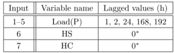
Table 1. Input variables for the HHNM model
Input Variable name Lagged values (h) 1–5 Load(P) 1, 2, 24, 168, 192
6 HS 0∗
7 HC 0∗
∗Lag 0 represents the hour to be forecast
4
The HHNM
The hierarchical hybrid neural model (HHNM) is shown in figure 1. It is made up of two distinct neural models — a hierarchical self-organizing model (HSOM), and a single-layer perceptron (SLP). The HSOM, in its turn, is made up of two self-organizing maps (SOMs). The HSOM features, performance, and potential are better evaluated in [2, 3].
HSOM
Time Integrator
Map Time Integrator
Λ Λ
Map Top
SOM
Bottom SOM SLP
V(t )
Figure 1. HHNM
The input to the model is a sequence in time ofm -dimensional vectors,S1 =V(1),V(2), . . . ,V(t), . . . ,
V(z), where the components of each vector are real values. The sequence is presented to the input layer of the bottom SOM, one vector at a time. The input layer hasmunits, one for each component of the input vector V(t), and a time integrator2. The activation
X(t) of the units in the input layer is given by
X(t) =V(t) +δ1X(t−1) (1)
where δ1 ∈ (0,1) is the decay rate. For each input vector X(t), the winning unit i∗(t) in the map is the
unit which has the smallest distance Ψ(i, t). For each output uniti, Ψ(i, t) is given by the Euclidean distance between the input vector X(t) and the unit’s weight vectorWi.
2
Time integrators act as memories for past events.
Each output unit i in the neighbourhood N∗(t) of
the winning uniti∗(t) has its weightWiupdated by
Wi(t+ 1) =Wi(t) +αΥ(i)[X(t)−Wi(t)] (2)
whereα∈(0,1) is the learning rate. Υ(i) is the neigh-bourhood interaction function [15], a Gaussian type function, and is given by
Υ(i) =κ1+κ2e−κ3[Φ(i,i ∗(t))]2
2σ2 (3)
where κ1, κ2, and κ3 are constants, σ is the radius of the neighbourhood N∗(t), and Φ(i, i∗(t)) is the
dis-tance in the map between the unit i and the winning uniti∗(t). The distance Φ(i′, i′′) between any two units
i′andi′′in the map is calculated according to the
max-imum norm,
Φ(i′, i′′) =max{|l′−l′′|,|c′−c′′|} (4)
where (l′, c′) and (l′′, c′′) are the coordinates of the
units i′ andi′′ respectively in the map.
The input to the top SOM is determined by the distances Φ(i, i∗(t)) of the n units in the map of the
bottom SOM. The input is thus a sequence in time of
n-dimensional vectors, S2 = Λ(Φ(i, i∗(1))), Λ(Φ(i, i∗(
2))), . . . ,Λ(Φ(i, i∗(t))), . . . ,Λ(Φ(i, i∗(z))), where Λ is
a n-dimensional transfer function on a n-dimensional space domain. Λ is defined as
Λ(Φ(i, i∗(t))) =
1−κΦ(i, i∗(t)) ifi∈N∗(t)
0 otherwise (5)
where κis a constant, and N∗(t) is a neighbourhood
of the winning unit.
The sequenceS2is then presented to the input layer of the top SOM, one vector at a time. The input layer hasnunits, one for each component of the input vector Λ(Φ(i, i∗(t))), and a time integrator. The activation X(t) of the units in the input layer is thus given by
X(t) = Λ(Φ(i, i∗(t))) +δ2X(t−1) (6)
whereδ2∈(0,1) is the decay rate.
The dynamics of the top SOM is identical to that of the bottom SOM.
The input to the SLP is also determined by the distances Φ(i, i∗(t)) of the p units in the map of the
top SOM. The input is thus a sequence in time of
p-dimensional vectors, S3 = Λ(Φ(i, i∗(1))), Λ(Φ(i, i∗(
2))), . . . ,Λ(Φ(i, i∗(t))), . . . ,Λ(Φ(i, i∗(z))), where Λ is
2500 2600 2700 2800 2900 3000 3100 3200
1 3 5
Load (MW)
Time (h)
Actual HSOM HHNM
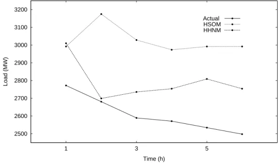
Figure 2. Actual load and forecast loads for February 05, 1995
The sequenceS3is then presented to the input layer of the SLP, one vector at a time. The input layer has
p units, one for each component of the input vector Λ(Φ(i, i∗(t))). The SLP is trained with the usual delta
rule [21, 20].
5
Experiments
The HHNM is required to foresee the time horizon from the first to the sixth hour. The training of its two SOMs takes place in two phases — coarse-mapping and fine-tuning. In the coarse-mapping phase, the learn-ing rate and the radius of the neighbourhood are re-duced linearly whereas in the fine-tuning phase, they are kept constant. The bottom and top SOMs were trained respectively with map sizes of 15×15 in 700 epochs, and 18×18 in 850 epochs. It was given the val-ues 0.4 and 0.7 to decay rates for the bottom and top SOMs, respectively. Several map sizes and decay rates were tested. The initial weights were given randomly to both SOMs.
The SLP holds a single unit in its output layer. Training was halted when the mean pattern error was 0.005. It was given the values 0.0001 and 0.9 to learn-ing rate and momentum respectively.
The training set comprised 2160 load patterns, span-ning ninety days. They were taken from November 1994 to January 1995. The maximum electric load fell around 3900 MWatts. There was no particular treat-ment for holidays.
Carpinteiro et al. [5] came up with two main con-clusions. First, the performance of HSOM3in STLF is
much superior than that of the multilayer perceptron (MLP). Second, the output mapping process employed on HSOM holds two weaknesses. These weaknesses resulted from the output mapping process employed. In this paper, we propose HHNM to avoid such weak-nesses by using a SLP model to perform the output mapping process.
The forecasts were then performed on the HSOM and HHNM models. A comparison of both models was carried out to verify whether or not HHNM outper-formed HSOM.
Figures 2 and 3 show the actual load and forecast load for two particular days. The first one — Sunday, February 05, 1995 — is a typical weekday, and the sec-ond one — Tuesday, February 07, 1995 — is a special weekday.
A typical weekday is one whose load patterns share some similarity with the load patterns of the same weekdays in former weeks. For instance, the load pat-terns for Tuesdays tend to display a similar behaviour. Yet, when an unexpected event, such as a holliday, hap-pens on one of those Tuesdays, it changes that fairly stationary behaviour. Such holliday is then said to be a special weekday. Special weekdays break down fore-casters, for they perform much better on typical than on special weekdays.
3
2600 2700 2800 2900 3000 3100 3200
1 3 5
Load (MW)
Time (h) Actual
HSOM HHNM
Figure 3. Actual load and forecast loads for February 07, 1995
Tables 2 and 3 present the performance of the fore-casters for one to six step ahead predictions on those weekdays, as well as the mean absolute percentage er-ror (MAPE).
Table 2. Hourly percentage error for February 05, 1995
Time (h) HSOM HHNM
1 7.92 8.58
2 18.43 0.68 3 16.96 5.65 4 15.65 7.12 5 18.05 10.83 6 19.77 10.25 MAPE (%) 16.13 7.19
The results from the HHNM are very promising. On the special day, the performances of HHNM and HSOM are similar. The results presented in figure 3 and ta-ble 3 show that HHNM yielded three better hourly per-centage errors, and three worse perper-centage errors than HSOM.
On the typical day, as shown in figure 2 and ta-ble 2, the performance of HHNM was significantly su-perior than that of HSOM. The hourly percentage er-rors yielded by HHNM were much better than that yielded by HSOM.
The superior performance displayed by HHNM
Table 3. Hourly percentage error for February 07, 1995
Time (h) HSOM HHNM
1 0.00 -0.63
2 1.31 -0.66
3 0.68 0.00
4 -0.67 -3.37
5 0.00 2.03
6 -1.34 -0.67
MAPE (%) 0.67 1.23
seems to be justified by its superior capacity to map output produced by the top SOM. As subsequent pre-dictions are based on the former ones, the enhanced mapping process provided by SLP yields to HHNM an overall higher performance.
6
Conclusion
The paper presents a novel artificial neural model to the problem of short-term load forecasting. The model has a topology made up of two self-organizing map networks — one on top of the other —, and a single-layer perceptron. It encodes and manipulates context information effectively.
Some conclusions may be drawn from the experi-ments. First, the knowledge representation proposed for the HHNM inputs seems to be adequate. It sup-plied the model with the necessary information to make it produce correct predictions.
Second, the HHNM performance on the forecasts was better than that of the HSOM, which, in its turn, is much better than that of the MLP. The results ob-tained have shown that the HHNM was able to perform efficiently the prediction of the electric load in short forecasting horizons.
Third, it is worth mentioning that MLP has been widely employed to tackle the problem of STLF so far. The results obtained thus suggest that HHNM may offer a better alternative to approach such problem.
A research and development project for a Brazilian electric utility is under course. The research will focus on the effects of the HHNM time integrators on the predictions in order to produce a better adaptability. Besides, it will focus on the study of its performance on larger load databases. The forecasts should also span a larger number of days in order to be more significant statistically.
Acknowledgements
This research is supported by CNPq, Brazil.
References
[1] A. Bakirtzis, et al. A neural network short-term load forecasting model for the Greek power system. IEEE Trans. on Power Systems, 11(2):858–863, May 1996. [2] O. A. S. Carpinteiro. A hierarchical self-organizing
map model for pattern recognition. InProceedings of the Brazilian Congress on Artificial Neural Networks (CBRN), pages 484–488, Florian´opolis, Brazil, 1997. [3] O. A. S. Carpinteiro. A hierarchical self-organizing
map model for sequence recognition. InProceedings of the ICANN, pages 815–820, Sk¨ovde, Sweden, 1998. [4] O. A. S. Carpinteiro. A hierarchical self-organizing
map model for sequence recognition.Pattern Analysis & Applications, 3(3):279–287, 2000.
[5] O. A. S. Carpinteiro, A. Reis, and A. da Silva. A hier-archical neural model in short-term load forecasting. Applied Soft Computing, 4:405–412, 2004.
[6] G. J. Chappell and J. G. Taylor. The temporal Koho-nen map. Neural Networks, 6:441–445, 1993.
[7] H. Hippert, C. Pedreira, and R. Souza. Neural net-works for short-term load forecasting: A review and evaluation.IEEE Trans. on Power Systems, 16(1):44– 55, Feb 2001.
[8] D. L. James and R. Miikkulainen. SARDNET: a self-organizing feature map for sequences. In Proceedings of the NIPS, volume 7, 1995.
[9] J. Kangas. On the Analysis of Pattern Sequences by Self-Organizing Maps. PhD thesis, Helsinki University of Technology, Finland, 1994.
[10] A. Khotanzad, R. Afkhami-Rohani, and D. Maratuku-lam. ANNSTLF – artificial neural network short-term load forecaster – generation three. IEEE Trans. on Power Systems, 13(4):1413–1422, Nov 1998.
[11] A. Khotanzad, R. Hwang, A. Abaye, and D. Maratukulam. An adaptive modular artificial neural hourly load forecaster and its implementation at electric utilities. IEEE Trans. on Power Systems, 10(3):1716–1722, August 1995.
[12] T. Kohonen. Self-Organizing Maps. Springer-Verlag, Berlin, third edition, 2001.
[13] K. Lee, Y. Cha, and J. Park. Short-term load forecast-ing usforecast-ing an artificial neural network.IEEE Trans. on Power Systems, 7(1):124–132, Feb 1992.
[14] K. Liu, S. Subbarayan, R. Shoults, M. Manry, C. Kwan, F. Lewis, and J. Naccarino. Comparison of very short-term load forecasting techniques. IEEE Trans. on Power Systems, 11(2):877–882, May 1996. [15] Z. Lo and B. Bavarian. Improved rate of convergence
in Kohonen neural network. In Proceedings of the IJCNN, volume 2, pages 201–206, July 8–12 1991. [16] O. Mohammed, D. Park, R. Merchant, T. Dinh,
C. Tong, A. Azeem, J. Farah, and C. Drake. Practical experiences with an adaptive neural network short-term load forecasting system. IEEE Trans. on Power Systems, 10(1):254–265, February 1995.
[17] H. Mori. State-of-the-art overview on artificial neural networks in power systems. In A Tutorial Course on Artificial Neural Networks with Applications to Power Systems, chapter 6, pages 51–70. IEEE Power Engi-neering Society, 1996.
[18] A. Papalexopoulos, S. Hao, and T. Peng. An imple-mentation of a neural network based load forecasting model for the EMS. IEEE Trans. on Power Systems, 9(4):1956–1962, Nov 1994.
[19] D. Park, M. El-Sharkawi, R. Marks II, L. Atlas, and M. Damborg. Electric load forecasting using an artifi-cial neural network. IEEE Trans. on Power Systems, 6(2):442–449, May 1991.
[20] R. S. Sutton and A. G. Barto. Toward a modern the-ory of adaptive networks: Expectation and prediction. Psychological Review, 88:135–170, 1981.