A Work Project, presented as part of the requirements for the Award of a Master’s Degree in Economics from the NOVA – School of Business and Economics

A Work Project, presented as part of the requirements for

the Award of a Master’s Degree in Economics from the

NOVA

–

School of Business and Economics

Estimating the Natural Interest Rate

for Italy and the Netherlands

Alexandre Duarte de Sousa Vale Mendonça

Student no. 792

A project carried on the Master’s in Economics Program under the

supervision of:

Professor Francesco Franco

ABSTRACT

Estimating the natural interest rate is fundamental for the proper definition of the stance of

monetary policy. This research applies the Kalman filter to jointly estimate the natural

interest rate, potential output and its growth rate for Italy and the Netherlands. The results

indicate a decreasing trend in the natural interest rates and point out that a single monetary

policy may not optimally suit both countries. There is a link between the real interest rate gap

and the output gap, and the estimates of the natural interest rate are subject to a high degree

of uncertainty.

Keywords: Kalman filter, Natural Interest Rate, Monetary Policy, Euro Area.

1. INTRODUCTION

Mainstream economic theories assume the existence of a long run equilibrium of the

economy where economic fundamentals such as the inflation rate or the output level reach a

level at which resources in the economy are optimally employed. Following the same line of

reasoning, the nominal interest rate is also assumed to converge to a natural level in the

long-run and this ‘equilibrium’ rate can be seen as a benchmark for monetary policy. The natural

interest rate (NIR) was first mentioned by Wicksell (1936) who described it as “a rate which

is neutral in respect to commodity prices, and tends neither to raise nor to lower them.”. Its

revival was driven by the works of Woodford (2003), who claimed that the equilibrium or

‘neutral’ rate addressed in the Taylor Rule varies continuously in response to real

disturbances. Therefore, the real interest rate gap, defined as the difference between the

actual interest rate and its natural counterpart, was seen as a good indicator for evaluating the

current stance of monetary policy, as opposed to measures that deal with monetary

aggregates or exchange rates.

nominal interest rate lies above the NIR, the policy is said to be contractionary and, by the

same reasoning, when the opposite happens, the policy is said to be expansionary. This link is

clearly illustrated by the Taylor Rule (Taylor, 1993), that makes recommendations for the

nominal monetary policy interest rate, based on current economic conditions, namely the

inflation gap and output gap, but also on the real interest rate. This type of monetary policy

rule provides an anchor for the behaviour of interest rates.

Long-term interest rates in most advanced economies have been particularly low since the

global financial crisis, something that has been linked with the current low short-term interest

rates (Rachel and Smith, 2015). By the line of reasoning previously mentioned, this would

mean that monetary policy was too expansionary. If this were the case, policy makers would

only need to adopt a more contractionary monetary policy, thus increasing the interest rates.

However, as mentioned by Blanchard, Furceri and Pescatori (2014) the problem is that this

‘looser monetary policy’ has not been accompanied by an increase in inflation and aggregate

demand, as predicted by economic theory, meaning that, despite being countercyclical, this

policy is not producing the desired outcome. Observable interest rates seem to be affected by

their equilibrium equivalents. Therefore, to understand what drives the current stance of

monetary policy, it is essential to comprehend the dynamics of its equilibrium aspects.

The subject of this research is to study the movements of the NIR for Italy and the

Netherlands, using the Kalman filter. The choice of these countries is related to the fact that

Italy is a large European country, usually considered a peripheral economy, and the

Netherlands is a strong economy of central Europe. These countries have different economic

indicators but belong to the same monetary union. Given the current context of low nominal

interest rates in the Euro Area and the ever-growing discussion regarding the future of the

single currency, it is fundamental to understand whether it makes sense for different

Stagnation hypothesis (Summers, 2014) increases the relevance of this type of discussion.

This analysis can be performed by a careful study of their equilibrium indicators.

The results seem to suggest that the Euro Area may not be such an optimal currency area,

given the differences in the estimates of the NIR. Secondly, this rate seems to be declining in

both economies, in accordance with the Secular Stagnation hypothesis. Finally, the estimates

of the NIR are subject to a high degree of uncertainty, in line with Laubach and Williams

(2003).

The remainder of this research is structured as follows: section 2 briefly discusses the

relevant literature on the topic; section 3 presents the model and the data; section 4 provides a

discussion of the results and compares with Holston, Laubach and Williams’ (2016) Euro

Area estimations; and the final section concludes.

2. LITERATURE REVIEW

Given the current goals of the central banks to achieve price stability and potential output, the

NIR is one of the key indicators of the stance of monetary policy (Amato, 2005). However,

there is no consensus regarding its measurement. This is mostly because this indicator “must

be inferred from the data, rather than directly observed” (Holston, Laubach and Williams,

2016). Several variables have been related to its measurement such as the time preference of

consumers, productivity and population growth, fiscal policy and risk-premia, and the

institutional structure of financial markets (ECB, 2004).

This concept is differentiated according to its time horizon. A strand of the literature claims

that the long-term NIR is the most stable, given the fact that in the long-run all markets have

cleared and, provided there are no new economic disturbances, all the growth rates in the

economy are constant, (Archibald and Hunter, 2001). Other authors prefer to study the

in all markets. Laubach and Williams (2003) refer to the short-term real interest rate as the

rate consistent with stable inflation and output at its potential level.

Neiss and Nelson (2001) were pioneers on the measurement of the NIR and its importance

for monetary policy decisions. In their perspective, the NIR is the real rate of return in an

economy with fully flexible prices. Using quarterly data for the United Kingdom for the

period between 1980 and 1999, they develop a Dynamic General Stochastic Equilibrium

(DSGE) with sticky prices and compute the ‘higher frequency component’ of the NIR, while

tracking its period-by-period movements, which are required to keep inflation constant.

Giammarioli and Valla (2003) apply a similar procedure to the Euro area, defining the NIR as

the rate that achieves period-by-period price stability. Both papers conclude that the real

interest rate gap can be quite helpful in predicting future inflation, in accordance with

Woodford (2003). As Larsen and Mckeown (2004) put it, a DSGE approach is preferable to

a Hodrick-Prescott (HP) approach or a Band-Pass (BP) approach in the sense that it allows

for a structural interpretation of the real interest rate gap and its variations. Nonetheless, this

approach relies on several arbitrary assumptions and its actual advantage over others is not

clear.

Brzoza-Brzenina (2003) argues that the NIR is a quite reliable indicator of monetary policy,

especially in an inflation-targeting regime. Through a Structural Vector Autoregressive

(SVAR) approach, the author estimates the NIR for the U.S. for the period between 1960 and

2001. He shows that this rate varies over time, being a procyclical variable, in the sense that

it increases during an economic expansion and decreases during recessions.

Orphanides and Williams (2002) try to study the impact of mismeasurements of the NIR in

monetary policy. Their study covers quarterly data for the U.S. for the period between 1969

and 2002, and assumes that the NIR follows a random walk. They estimate the NIR using

only account for the information available at time t to compute estimates of unobservable

variables) and two-sided estimates (which account for all the information available in the

sample, both past and future, to compute estimates of a variable at time t), and multivariate

filters, such as the Kalman filter (which produces optimal linear future forecasts based on

information up to time t). They conclude that underestimating the volatility of real-time

estimates of the NIR may be quite costly in terms of economic stabilization. On top of this,

they claim that the costs of underestimating mismeasurements of this rate are higher than the

costs of overestimating them.

In a 2003 paper, Laubach and Williams applied a State-Space approach to jointly estimate

highly persistent components of the NIR, potential output and its trend growth rate in the

U.S. for the period between 1961 and 2002. From their point of view, the NIR is the real

short-term interest rate consistent with output at its potential level and stable inflation in the

medium-term, i.e. once the effects of demand shocks on the output gap and supply shocks on

inflation have completely vanished. Their approach builds on the works of Watson (1986),

Clark (1987) and Kuttner (1994), with a key difference in that these authors do not account

for an explicit relationship between the NIR and the growth rate of potential output. Their

work resembles a New Keynesian framework (Galí, 2008), in the sense that they use a

Phillips curve and an intertemporal IS curve to describe the dynamics of both the output gap

and the inflation rate as a function of the real interest rate gap. However, the authors depart

from the conceptual DSGE approach given that they do not treat the growth rate of

technology and the rate of time preference as fixed. Laubach and Williams allow the NIR to

be affected by low-frequency nonstationary processes that are highly persistent but difficult

to detect. The authors estimate several variants of the IS and Phillips curve by maximum

likelihood using the Kalman filter and conclude that the NIR shows significant variation over

potential output. Once again, they state that it is important to account for mismeasurements in

computing natural rates when making monetary policy decisions. In 2016, the authors

updated the previous analysis, using data from the U.S., Canada, the Euro Area and the

United Kingdom. Even though the conclusions are the same as in the 2003 paper, the authors

emphasize the decline observed in the NIRs over the past quarter century, reaching a

historically low point, and corroborating the Secular Stagnation hypothesis.

The issue of the reliability of the estimates of the NIR is also addressed by Clark and Kozicki

(2004), who claim that these estimates are easily distorted by different data sources,

successive data revisions and the usage of one-sided filters. Using the same approach as

Laubach and Williams (2003), they conclude that the NIR is closely linked with the growth

rate of potential output. On top of this, they also model the NIR as a random walk, as in

Orphanides and Williams (2002), compare both models and reinforce the fact that these

estimates should be carefully dealt with.

Garnier and Wilhelmsen (2005) use the same procedure as Laubach and Williams (2003),

thus applying the Kalman filter to a small-scale macroeconomic model, which encompasses

an IS and a Phillips curve, in order to estimate the NIR for Germany, the U.S. and the Euro

Area. To do so, they use quarterly data for the period between 1961 and 2004 and conclude

that the real interest rate gap is negatively correlated with the output gap and inflation.

Besides pointing out the fact that one must be careful with the uncertainty regarding these

estimations, the authors also conclude that the real interest rate gap may contain important

information regarding future inflation in the Euro area.

Mésonnier and Renne (2007) depart from the same model as Laubach and Williams (2003)

but instead assume that the unobservable process that drives the low frequency common

fluctuations of the NIR and the growth of potential output is a stationary autoregressive

co-movements between the NIR and the growth rate of potential output. Furthermore, they

compute an ex-ante real interest rate, opting for the usage of the inflation expectations

provided by the model instead of deriving them from an autoregressive process. Applying

this methodology to the Euro area for the period between 1979 and 2002, they estimate a

time-varying NIR and conclude that monetary policy has been adequate for stabilising

European inflation.

Benati and Vitale (2007) use the Kalman filter to jointly estimate the NIR, the natural rate of

unemployment, expected inflation and potential output in the Euro Area, the U.S., Australia,

Sweden and the United Kingdom. The authors generate the expectation of inflation

endogenously within the model and exploit the information contained in the unemployment

gap, to better filter out the cyclical component of economic activity. Apart from this, their

approach is quite similar to the one performed by Laubach and Williams (2003). They

conclude that the time-variation in the NIR is estimated to be quite large for the U.S., the

Euro Area and Sweden, and smaller for Australia and the United Kingdom. Moreover, the

authors also strengthen the idea that estimations of the NIR are subject to a high degree of

uncertainty.

Lubik and Matthes (2015) make a comparison between the Laubach and Williams approach

and a Time-Varying Parameters VAR (TVP-VAR) approach. The latter allows the lag

coefficients (the parameters of the model) to vary over time. Applying both models to the

same US quarterly data for the period between 1961 and 2015, the authors claim that the

Laubach and Williams’ estimates vary considerably and have high standard errors. They

claim that these effects could be softened by increasing the theoretical rigor of the model or,

on the other hand, reducing its structural aspects. According to the authors, besides the

sustained decrease observed in the real rate as well as in its natural counterpart, the real rate’s

could be more adequate for the study of the NIR since it imposes a less strict economic

structure, meaning that it just captures the co-movement between the variables in a flexible

manner. Nonetheless, the authors conclude that both models yield similar estimates since the

1980s and the uncertainty regarding these estimates makes the models practically indifferent

over the past 30 years. However, they note that the natural counterpart has been above the

real rate over an extended period, something that has been proven by both models.

This research contributes to the existing literature by applying the same procedure as

Laubach and Williams (2003) to data for Italy and the Netherlands in order to jointly estimate

the output gap, the growth rate of potential output and the NIR.

3. DISCUSSION OF THE TOPIC 3.1. Model

The approach adopted in this research follows Laubach and Williams (2003) (LW). The NIR

is the real rate consistent with stable inflation and output at its potential level, as in Wicksell

(1936). This research builds on a New Keynesian framework in the sense that an

intertemporal IS curve and a Phillips curve are used to study the dynamics of the output gap

and inflation as a function of the real interest rate gap, following the DSGE literature. As

previously mentioned, the LW approach differs from the standard DSGE models since it

allows for parameters that are usually treated as fixed in the literature (such as the

households’ rate of time preference or the productivity growth) to be affected by highly

persistent and difficult-to-detect fluctuations (Stock and Watson, 1998). Therefore, the model

allows the NIR to be affected by low-frequency nonstationary processes (i.e. shocks that

affect the output gap and inflation but not the NIR).

To reduce the risks associated with misspecifications in the output gap and inflation

dynamics, the estimations are performed using reduced-form equations. Given this, the

(𝟏)𝑦𝑡 = 𝑦𝑡𝑇+ 𝛼1(𝑦𝑡−1− 𝑦𝑡−1𝑇 ) + 𝛼2(𝑦𝑡−2− 𝑦𝑡−2𝑇 ) +_{200 [}𝛼𝑟 (𝑟𝑡−1− 𝑟𝑡−1∗ ) + (𝑟𝑡−2− 𝑟𝑡−2∗ )]

+ 𝜀_𝑡𝑦

(𝟐) 𝜋𝑡= 𝛽𝜋𝜋𝑡−1+(1 − 𝛽₃ 𝜋)𝜋𝑡−2+(1 − 𝛽₃ 𝜋)𝜋𝑡−3+(1 − 𝛽₃ 𝜋)𝜋𝑡−4+ 100𝛽𝑦(𝑦𝑡−1− 𝑦𝑡−1𝑇 )

+ 𝜀𝑡𝜋

(𝟑) 𝑟𝑡∗ = 𝑔𝑡 + 𝑧𝑡

(𝟒) 𝑧𝑡 = 𝑧𝑡−1+ 𝜀𝑡𝑧

(𝟓) 𝑦𝑡𝑇 = 𝑦𝑡−1𝑇 + 𝑔𝑡−1+ 𝜀𝑡𝑇

(𝟔) 𝑔𝑡 = 𝑔𝑡−1+ 𝜀𝑡𝑔

Equations (1) and (2) are the measurement equations of the State-Space model, linking the

observed variables (𝑦_𝑡 and 𝜋_𝑡) to the unobserved variables (𝑦_𝑡𝑇 and 𝑟_𝑡∗). Equation (1), the intertemporal IS curve, relates the output gap, 100(𝑦_𝑡− 𝑦_𝑡𝑇), i.e. the log deviation of GDP (𝑦_𝑡) from its potential level (𝑦_𝑡𝑇), to its own lags and to the lags of the real interest rate gap (the difference between the real interest rate, 𝑟_𝑡, and its natural counterpart, 𝑟_𝑡∗). The sum of the coefficients 𝛼₁ and 𝛼₂ reflects the persistence of the output gap, meaning that the higher their sum, the greater will be the intertemporal dependence of current output gap. The

coefficient 𝛼_𝑟 is the slope of the IS curve and it is expected to be negative, given that economic theory predicts that a positive real interest rate gap is associated with a negative

output gap1_{. In case the former gap is equal to zero and there are no demand shocks (}𝜀

𝑡𝑦 = 0),

the output gap converges to zero, meaning that output will be equal to its equilibrium level in

the long-run. Equation (2) is the backward-looking Phillips curve and it explains inflation, 𝜋_𝑡, as a function of its own lags (the first lag and an average of the second to fourth lags) and the

lagged output gap. As in LW, the restriction that the coefficients of all the terms of lagged

inflation sum to 1 is imposed2_{. The coefficient} 𝛽

𝑦 is the slope of the Phillips curve and it is

1 _{The choice of two lags of the output gap and two gaps of the real interest rate gap is in line with LW. The restriction that the two lags of}

the real interest rate gap have the same coefficient is not rejected by a Wald test.

expected to be positive since a positive output gap creates inflationary pressures on the

economy.

Equations (3) to (6) are the transition equations of the State-Space model. Equation (3) is the

law of motion of the NIR, modelling the NIR as a linear combination of the growth rate of

potential output, 𝑔_𝑡, and all the other determinants of 𝑟_𝑡∗, such as changes in the population growth rate or the discount rate (Guarda, Rouabah and Wintr, 2005), captured by the term 𝑧_𝑡. As in LW, this research assumes a one-for-one relationship between the NIR and the growth

rate of potential output. For simplicity, 𝑧_𝑡 is assumed to follow a random walk process, described by equation (4).

Potential output, 𝑦_𝑡𝑇, is assumed to follow a random walk process with a stochastic drift, 𝑔_𝑡 i.e. the growth rate of potential output (equation (5)), which itself follows a random walk,

displayed in equation (6). This implies that an innovation 𝜀_𝑡𝑇 has a permanent effect on the level of potential output but only a one-period effect on its growth rate, whereas an

innovation 𝜀_𝑡𝑔 has a permanent effect on the growth rate of potential output, implying that potential output is integrated of order 2, as in Holston, Laubach and Williams (2016).

𝜀𝑡𝑇, 𝜀𝑡𝑔 and 𝜀𝑡𝑧 are assumed to be normally independently distributed shocks with standard

deviations 𝜎_𝑇, 𝜎_𝑔 and 𝜎_𝑧 respectively and are serially and contemporaneously uncorrelated.

3.2. Data

The computation of the NIR requires data for real GDP, inflation, a procedure to calculate

inflation expectations and the short-term nominal interest rate, in order to obtain the ex-ante

real short-term interest rate.

The real GDP measure chosen is the Index of Real Gross Domestic Product, Seasonally

Adjusted from the IMF International Financial Statistics. The measure of inflation is

constructed using the consumer price index excluding food and energy, also known as core

In their 2003 paper, Laubach and Williams computed inflation expectations through a

univariate AR(3) process of inflation estimated over the past 40 quarters to generate a

forecast of four-quarter-ahead inflation. However, for reasons of consistency, the proxy

chosen for inflation expectations is a four-quarter moving average of past inflation, as in

Holston, Laubach and Williams (2016).

Both Italy and the Netherlands are on a monetary union since 1999 and, as consequence,

there is no long series for the short-term nominal monetary policy interest rate. Therefore,

this rate was proxied by the 3-month interbank rate as in Manrique and Marqués (2004). The

authors argue that this rate, despite “being closely linked to the monetary policy interest rate,

has a greater variability than the latter, which makes for readier estimation”. This series was

retrieved from the OECD. The ex-ante real short-term interest rate is the difference between

the short-term nominal interest rate and the inflation expectations.

Given data availability of the 3-month interbank rate, data for Italy is composed by 143

quarters ranging from 1980:Q1 to 2016:Q3, whereas for the Netherlands, the sample is

composed by 119 quarters ranging from 1986:Q1 to 2016:Q3. The series were seasonally

adjusted using the R-packages ‘seasonal’ and ‘x13binary’. The results of the

Augmented-Dickey Fuller test can be found in Table 1 in Appendix 2.

3.3. Empirical Implementation

As it was previously mentioned, this research applies the Kalman filter to jointly estimate the

level of potential output, its growth rate, and the NIR. This is done by rewriting equations (1)

to (6) in the State-Space form and estimating them by maximum likelihood3_.

A widely discussed issue in the literature related to this type of maximum likelihood

estimations is the ‘pile-up problem’ (Stock, 1994). As clarified by Roberts (2001), 20th

century U.S. data suggests that the growth rate of potential output may vary over time but

these variations are likely to be small relative to the overall variation in the series, meaning

that it may be difficult to detect them in the data. The problem comes from the fact that if a

variable has large shocks to its level, but only small shocks to its change, the usual maximum

likelihood estimation procedures will tend to obtain standard deviations of the shocks to the

change of zero, even though that may not be the case. In this particular case, the standard

deviations of the innovations to 𝑧 and the growth rate of potential output (𝜀_𝑡𝑧 and 𝜀_𝑡𝑔) will be biased towards zero. This problem has been addressed by Stock and Watson (1998),

proposing a technique, the median unbiased estimator, which is shown to better capture the

true size of small shocks to the growth rate of potential output than maximum likelihood

estimation4_{. Basically, the authors propose a median-unbiased estimator of the signal-to-noise}

ratios 𝜆_𝑔 = 𝜎_𝑔/𝜎_𝑇 and 𝜆_𝑧 = 𝜎_𝑧×𝛼_𝑟/𝜎_𝑦. These ratios are imposed when estimating the remaining model parameters by maximum likelihood, i.e. 𝛼₁, 𝛼₂, 𝛼_𝑟, 𝛽_𝜋, 𝛽_𝑦, 𝜎_𝑦, 𝜎_𝜋 and 𝜎_𝑇. The estimation approach can be decomposed in three sequential steps. In the first step, the

methodology of Kuttner (1994) is adopted and the Kalman filter is used to estimate potential

output, omitting the real interest rate gap from equation (1) and assuming that the growth rate

of potential output (𝑔_𝑡) is constant. This is equivalent to ommiting equations (4) and (5). The exponential Wald statistic of Andrews and Ploberger (1994) for a structural break with

unknown break date is computed on the first difference of the estimated potential output, to

obtain the median unbiased estimate of 𝜆_𝑔.

In the second stage, the ratio 𝜆_𝑔 is imposed and the Kalman filter is applied again, this time including the real interest rate gap in equation (1) and assuming that 𝑧_𝑡 is constant, so that 𝑔_𝑡

4 _{The authors depart from the idea that if there is a shock to the growth rate of potential output, then if one were to run a test looking for the}

is no longer constant. Once again, the exponential Wald test is performed, this time for an

intercept shift in the output gap equation at an unknown date, to obtain an estimate of 𝜆_𝑧. In the third stage, the estimates of 𝜆_𝑔 and 𝜆_𝑧 are imposed and the remaining parameters of the model are estimated by maximum likelihood, as in Harvey (1989). It is important to

notice that Holston, Laubach and Williams (2016) impose constraints on the slopes of the IS

curve and the Phillips curve. In fact, they impose that 𝛼_𝑟 must be negative and 𝛽_𝑦 must be positive5_{, in accordance with economic theory. Given that the authors claim these are}

minimal constraints to facilitate the convergence of the optimization of the model, they are

also imposed in this research.

4. RESULTS

4.1. Parameter Estimates

Estimation results are reported in Table 2 in Appendix 2. The value of 𝜆_𝑔 is quite similar for both economies (0.038) and seems to indicate a small time-variation in the estimates of the

growth rate of potential output. This value is close to the Holston, Laubach and Williams’

(2016) (HLW) Euro Area estimate of 0.030. However, the values of 𝜆_𝑧 are quite different between countries (0.041 for Italy, 0.122 for the Netherlands and 0.042 for the HLW Euro

Area estimation). This suggests that the time variation of the NIR is greater for the

Netherlands, something that is confirmed by the smaller value of 𝛼_𝑟 for this economy. Besides this, the uncertainty regarding the estimates of the NIR seem to be related to the

statistical significance of both 𝛼_𝑟 and 𝛽_𝑦. These coefficients are not statistically significant for the Netherlands and, in fact, the average standard errors of both the NIR and potential

output are relatively greater than those of Italy.

5 _{More specifically, the authors impose that 𝛼}

It is also important to notice that the output gap is estimated to be less persistent in Italy, due

to the smaller value of 𝛼₁+ 𝛼₂, but inflation in Italy is more affected by these temporary fluctuations in the output gap, given its higher 𝛽_𝑦.

The results seem to suggest that both the output gap and the real interest rate gap are well

identified for the case of Italy, given the slope coefficients of 𝛼_𝑟 and 𝛽_𝑦. However, it is important to notice that there is some imprecision in the estimates of the NIR, given the

sample average standard error of 1.787 percentage points. These mismeasurement issues are

even greater when looking at the one-sided estimates, which, by using only current and past

observations in estimating the state, are a better proxy for “real-time estimates”. As it is

possible to see, the final observation standard errors (representing the one-sided estimates’

mismeasurement when the true values of 𝜆_𝑔 and 𝜆_𝑧 are assumed to be known) are even greater. This effect is amplified for the Netherlands.

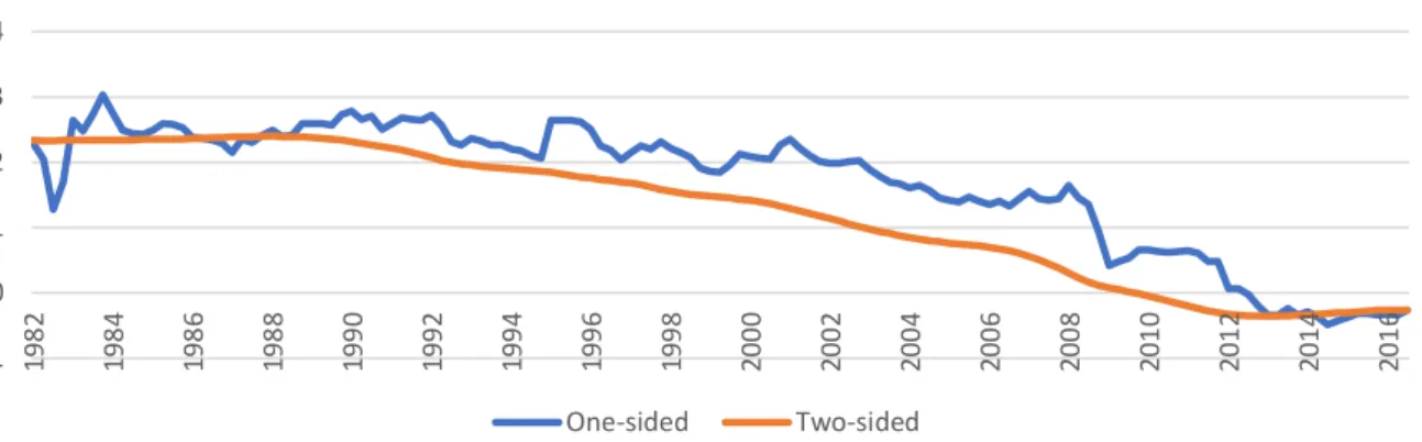
Figure 16 _{plots the filtered (one-sided) estimate of the natural rate of interest and its smoothed}

(two-sided) estimate for Italy. It is clear that the two-sided estimates are smoother, which can

be explained by the fact that these account for all the information available in the sample,

past and future, to compute current estimates of a variable, i.e. they recursively update their

estimates based on previous estimates. The same analysis is true for the case of the

Netherlands, displayed in Figure 2. Both figures demonstrate a pattern of declining NIRs,

decreasing at a faster pace after 2007, confirming the Secular Stagnation hypothesis.

4.2. Estimates of the Output Gap, Real Interest Rate Gap and the Growth Rate of Potential Output

Figures 3 and 4 show the one-sided estimates of the output gap and the real interest rate gap

for both economies. The shaded regions indicate the Euro Area recession periods7_{. As one}

would expect, apart from a few exceptions, output gap moves downwards in periods of

recessions and, in fact, has remained negative since the financial crisis. On the other hand, the

real interest rate gap moves in the inverse direction of output gap, meaning that a negative

real interest rate gap is usually accompanied by increases in the output gap and vice-versa. In

the case of Italy, until the late 1990’s, the real interest rate gap is quite large, which is

reflected on a negative output gap, but around 2000, after the introduction of the single

currency, the former gap becomes more stable around zero, yielding a similar effect on the

output gap, which becomes positive and stable. In the Dutch case, the real interest rate gap

does not stabilise around zero after 2000. In fact, it becomes more volatile and larger,

something that turns the output gap negative.

Figures 5 and 6 suggest an even more interesting result. These display the estimates of the

NIR and the growth rate of potential output for Italy and the Netherlands, respectively. In

fact, both figures seem to be in accordance with the Secular Stagnation hypothesis (Summers,

2014) – the idea that the economy is stagnating for the past 20 years, observed through the

decrease in inflation, interest rates and growth rates of the economy. The NIR has been

declining in Italy for the past 20 years and this process appears to have accelerated after the

2008 financial crisis reaching a negative value in 2012. The same is true for the Netherlands

but the results suggest that the NIR has been negative since 2003, increasing from 2006 to

2007 (becoming positive) and turning negative again following the financial crisis.

The growth rate of potential output has moved in a quite similar fashion as the NIR in Italy,

also experiencing a downward trend since 2008. However, curiously, it has remained quite

4.3. Comparing with HP Filter

A detailed analysis of Table 2 seems to corroborate the initial idea that one must be careful

with any estimate of the NIR, given the already mentioned imprecision of the Kalman filter

estimates. Therefore, this section compares these estimates with those from a univariate filter.

Since the results for Italy are better suited for a statistical analysis (the coefficients are

statistically significant and the standard errors are friendlier), the Netherlands will not be

addressed in this section.

Figure 7 plots the proxy for the ex-ante real interest rate (described in the data section), the

two-sided estimate of the NIR, its one-sided estimate and the NIR estimated through a

univariate filter. More specifically, the univariate filter used is the Hodrick – Prescott (1997)

(HP) filter, with a smoothing parameter 𝜆 of 6400, following Laubach and Williams (2003). This parametrization is chosen so that the resulting estimates correspond to the

low-frequency components, like the Kalman filter.

Given the fact that the univariate estimates are two-sided weighted averages by nature, they

tend to be quite close to the actual rate and, consequently, do not capture the effects of

movements in inflation. Until the early 1990’s, the univariate estimate is quite close to the

actual rate even though there was a considerable decrease in inflation during that period. On

the other hand, the Kalman filter estimates (both the one-sided and the two-sided estimates)

show little movement of the NIR during periods of volatile inflation (such as the one that

lasted until the late 1990’s). Therefore, the Kalman filter approach seems to be more capable

of estimating lower-frequency movements in the NIR than the univariate method.

As Orphanides and Williams (2002) put it, univariate filters “separate the cyclical component

of a series from its secular trend and use the latter as a proxy for the natural level of the

detrended series”, which makes them extremely easy to implement. On the other hand,

they recursively update their estimations, i.e. they make an initial prediction of the states

based on initial information which is then updated based on the outcome of the following

estimation. Therefore, they can provide more accurate estimates.

Univariate filters have difficulty in making a clear distinction between the secular and

cyclical fluctuations of a series, meaning that the greater the dataset is, the more accurate

these estimates will be. This problem is not so present in multivariate filters because, in this

case, the estimates of the NIR are updated based on inflation surprises (only real-time

information is used).

To sum up, given their higher complexity and accuracy, multivariate filters such as the

Kalman filter, seem to be better suited for performing real-time estimates of the NIR.

However, one must be careful when making such conclusion because these filters perform

under the premise that the low-frequency components’ behaviour is well modelled,

something that may not necessarily be true, thus turning the multivariate estimations false.

4.4. Estimates of the Natural Interest Rate

Figure 8 plots the one-sided estimates of the NIR for Italy and the Netherlands, as well as the

one-sided estimates performed by Holston, Laubach and Williams (2016) for the Euro Area.

It is important to mention that Italy and the Netherlands share the same currency since 1999.

According to Mundell (1961), the optimality of an Optimum Currency Area (OCA) depends

on the importance of asymmetric shocks within the union but also in the existence of

adjustment mechanisms to tackle them. The Euro Area is currently composed by 19

countries, with different growth rates, inflation rates and unemployment rates so that one can

say that the Euro Area is a very heterogeneous monetary union. On top of this, as De Grauwe

(2003) points out, since it is a quite large group, there is a higher probability of occurrence of

asymmetric shocks. Given that a monetary union implies a single interest rate set by a single

countries. This issue was also raised by Moons and Van Poeck (2008) who claimed that,

before the 2004 Euro Area enlargement, the interest rate set by the ECB (Main Refinancing

Operations rate – MRO) did not fit all the monetary union countries in an equal manner.

Consequently, the single rate tends to be closer to the needs of the larger countries, such as

Germany, France, Italy and Spain, which represent more than 50% of the total Euro Area

GDP. Nechio (2011) and Darvas and Meller (2013), using a simple Taylor-rule function,

showed that even though the MRO was in line with the recommendation for the Euro Area as

a whole, once they decomposed the countries into two distinct groups, the actual rate was

closer to the recommendation for the core group (Austria, Belgium, Finland, France,

Germany, Italy and The Netherlands) than for the periphery group (Greece, Ireland, Portugal

and Spain), implying that the single interest rate does not seem to be optimal. This also

means that for countries such as Germany the current stance of monetary policy may be too

loose.

Following this line of reasoning, it would be expectable that countries that belong to a

monetary union share similar economic indicators but would also be similar on their

fundamentals, i.e. NAIRU, potential output and the NIR. By looking at the graph, one can see

that estimates for the Euro Area and those for Italy and the Netherlands start diverging at a

faster pace in the late 1990’s, during the implementation of the single currency. This may

contradict the claim by Frankel and Rose (1998) that more integration promotes more

business cycle correlation. Curiously enough, the estimates for Italy and the Euro Area seem

to converge during the 2008 financial crisis, diverge afterwards, and converge again in 2015.

The main point here is that Italy and the Netherlands have widely different NIRs between

themselves and different from those of the Euro Area, thus suggesting that a single nominal

interest rate may not be advisable since this group of countries is fairly heterogeneous, even

one should once again mention that these estimates are subject to a high degree of uncertainty

and are quite dependent on the specifications of the model so that any inference and

conclusions must be dealt with caution.

Besides this, Figure 8 shows that the equilibrium interest rates have been decreasing in all the

mentioned economies, reaching negative values. In the case of Italy, the growth rate of

potential output has followed this negative trend, seeming to embody the ‘Secular Stagnation’

hypothesis.

5. CONCLUSION

The ability of the European Central Bank to adopt policies that can satisfy all the Euro Area

members has been under discussion given these countries’ different economic characteristics.

In this research, the methodology of Laubach and Williams (2003) was applied to jointly

estimate the output gap, the growth rate of potential output and the NIR for Italy and the

Netherlands.

The findings suggest that the ‘Wicksellian’ rate of interest in these economies has been

declining for the past 20 years, reaching a negative point. This idea corroborates the results of

Holston, Laubach and Williams (2016), who observed a similar phenomenon for Canada, the

Euro Area, the United Kingdom and the United States. In line with the authors, these

estimates are also subject to a high degree of uncertainty.

A lower average real interest rate implies that episodes, such as the current one in the Euro

Area, of “monetary policy being constrained at the effective zero lower bound are likely to be

more frequent and longer” (Laubach and Williams, 2016). Therefore, this research results can

help policymakers on their decisions regarding future monetary policy, as central bankers can

respond to this, for instance, by increasing the inflation objective, or by allowing nominal

Since the sustained decline in the NIR seems to be an international phenomenon, more

research ought to be made on the drivers of this rate to improve the credibility of these

estimates. The analysis of this research could be repeated for the other Euro Area countries,

studying their business cycles and checking whether the monetary union is in fact optimal or

not, given their fundamentals. Furthermore, this should inform a discussion on the limits of

monetary policy.

6. REFERENCES

• Amato, Jeffrey D. 2005. “The role of the natural rate of interest on monetary policy.”

BIS Working Papers 171.

• Andrews, Donald and Werner Ploberger. 1994. “Optimal Tests When a Nuisance Parameter is Present Only Under the Alternative.” Econometrica, 62: 1383-1414.

• Archibald, Joanne, and Leni Hunter. 2001. “What is the neutral interest rate, and how can we use it?” Reserve Bank of New Zealand, Bulletin vol.64, 3.

• Benati, Luca, and Giovanni Vitale. 2007. “Joint Estimation of the Natural Rate of

Interest, the Natural Rate of Unemployment, Expected Inflation and Potential

Output.” European Central Bank Working Paper Series 797.

• Blanchard, Olivier, Davide Furceri, and Andrea Pescatori. 2014. “A Prolonged Period of Low Real Interest Rates?”, in Coen Teulings and Richard Baldwin (eds) ‘Secular

Stagnation: Facts, Causes and Cures’, CEPR Press: 101-110.

• Brzoza-Brzezina, Michal. 2003. “Estimating the Natural Rate of Interest: a SVAR

approach.” National Bank of Poland, 27.

• Clark, Peter. 1987. “The Cyclical Components of U.S. Economic Activity.” Quarterly Journal of Economics, 102: 797-814.

• Clark, Todd E., and Sharon Kozicki. 2004. “Estimating Equilibrium Real Rates in

Real-time.” Deutsche Bundesbank Discussion Paper Series, 32.

• Darvas, Zsolt, and Silvia Merler. 2013. “-15% to +4%: Taylor-rule Interest Rates for

Euro Area Countries.” Bruegel, September 18. http://bruegel.org/2013/09/15-to-4-taylor-rule-interest-rates-for-euro-area-countries/.

• De Grauwe, Paul. 2003. “The Euro at Stake? The Monetary Union in an Enlarged Europe.” CESifo Economics Studies, 49: 103-121.

• ECB. 2004. “The Natural Real Interest Rate in the Euro Area.” European Economic Bulletin, 5(04).

• Frankel, Jeffrey A., and Andrew K. Rose. 1998. “The Endogeneity of Optimum Currency Areas Criteria.” The Economic Journal 108 (449): 1009-1025.

• Galí, Jordi. 2008. Monetary Policy, Inflation, and the Business Cycle: An introduction to the New Keynesian Framework. Princeton, NJ: Princeton University Press.

• Garnier, Julien, and Bjorn-Roger Wilhelmsen. 2005. “The Natural Real Interest Rate

and the Output Gap in the Euro Area: A joint estimation.” European Central Bank

Working Paper Series 546.

• Guarda, Paolo, Abdelaziz Rouabah, and Ladislav Wintr. 2005. “Estimating the NIR

for the Euro Area and Luxembourg.” Banque Centrale du Luxembourg Working

Paper 15.

• Harvey, Andrew C. 1989. Forecasting, Structural Time Series Models and the Kalman Filter. Cambridge: Cambridge University Press.

• Hodrick, Robert J., and Edward C. Prescott. 1997. “Post-war Business Cycles: an

Empirical Investigation.” Journal of Money, Credit and Banking, 29: 1-16.

• Holston, Kathryn, Thomas Laubach, and John C. Williams. 2016. “Measuring the

Natural Rate of Interest: International Trends and Determinants.” Federal Reserve

Bank of San Francisco Working Paper 2016-11.

• Kuttner, Kenneth. 1994. “Estimating Potential Output as a Latent Variable.” Journal of Business and Economic Statistics, 12(3): 361-368.

• Larsen, Jens D. J., and Jack Mckeown. 2004. “The Informational Content of Empirical Measures of Real Interest Rate and Output Gaps for the United Kingdom.”

Bank of England Working Paper 224.

• Laubach, Thomas, and John C. Williams. 2003. “Measuring the Natural Rate of

Interest.” The Review of Economics and Statistics, 85(4): 1063-1070.

• Laubach, Thomas, and John C. Williams. 2016. “Measuring the Natural Rate of Interest Redux.” Business Economics, 51: 257-267.

• Lubik, Thomas A., and Christian Matthes. 2015. “Calculating the Natural Rate of

Interest: A Comparison of Two Alternative Approaches.” Federal Reserve Bank of

Richmond Economic Brief 15-10.

• Manrique, Marta, and José Manuel Marqués. 2004. “An Empirical Approximation of

the Natural Rate of Interest and Potential Growth.” Banco de España Documentos de Trabajo 0416.

• Mésonnier, Jean-Stéphane, and Jean-Paul Renne. 2007. “A Time-Varying Natural

Rate of Interest for the Euro Area.” European Economic Review, 51: 1768-1784

• Moons, Cindy, and André Van Poeck. 2008. “Does one size fit all? A Taylor-rule

based analysis of monetary policy for current and future EMU members.” Applied Economics, Taylor & Francis (Routledge), 40(02): 193-199.

• Mundell, Robert A. 1961. “A Theory of Optimum Currency Areas.” The American Economic Review, 51(4): 657-665.

• Nechio, Fernanda. 2011. “Monetary Policy When One Size Does Not Fit All.”

FRBSF Economic Letter 2011-18.

• Neiss, Katharine S., and Edward Nelson. 2001. “The Real Interest Rate Gap as an

Inflation Indicator.” CEPR Discussion Paper Series, 2848.

• Orphanides, Athanasios, and John C. Williams. 2002. “Robust Monetary Policy Rules with Unknown Natural Rates.” Federal Reserve Bank of San Francisco Working

Paper 2003-01.

• Rachel, Lukasz, and Thomas D. Smith. 2015. “Secular Drivers of the Global Real

Interest Rate.” Bank of England Staff Working Paper 571.

• Roberts, John M. 2001. “Estimates of the Productivity Trend Using Time-Varying

Parameter Techniques.” The B.E. Journal of Macroeconomics, 1.

• Stock, James H. 1994. “Unit Roots, Structural Breaks and Trends.”, in R. Engle and

D. Macfadden (eds) ‘Handbook of Econometrics,’ Vol. 4, Amsterdam, Elsevier

Science, 2739-2841.

• Stock, James H., and Mark W. Watson. 1998. “Median Unbiased Estimation of

Coefficient Variance in a Time-Varying Parameter Model.” Journal of the American

• Summers, Lawrence H. 2014. “Reflections on the ‘New Secular Stagnation

Hypothesis’.”, in Coen Teulings and Richard Baldwin (eds) ‘Secular Stagnation:

Facts, Causes and Cures’, CEPR Press: 27-40.

• Taylor, John B. 1993. “Discretion versus Policy Rules in Practice.” Carnegie-Rochester Conference Series on Public Policy, 39: 195-214.

• Watson, Mark W. 1986. “Univariate Detrending Methods with Stochastic Trends.” Journal of Monetary Economics, 18: 49-75.

• Wicksell, Knut. 1936. Interest and Prices (translated by R.F. Kahn). London: Macmillan.

• Woodford, Michael. 2003. Interest and Prices: Foundations of a Theory of Monetary Policy. Princeton: Princeton Univesity Press.

APPENDIX 1 – State-Space Representation

To estimate the Kalman filter, equations (1) to (6) must be rewritten in State-Space form:

(1) 𝑌_𝑡 = 𝐴. 𝑥_𝑡+ 𝐻. 𝛾_𝑡+ 𝑣_𝑡 (2) 𝛾_𝑡 = 𝐹. 𝛾_𝑡−1+ 𝜀_𝑡

where 𝑌_𝑡 is a vector of contemporaneous endogenous observed variables, 𝑥_𝑡 is a vector of exogenous and lagged exogenous variables, and 𝛾_𝑡 is a vector of unobserved states. The matrices A, H and F are the coefficient matrices. The vectors 𝑣_𝑡 and 𝜀_𝑡 are the stochastic disturbances and are assumed to be Gaussian and mutually uncorrelated, with mean zero and

variance-covariance matrices R and Q, respectively. Matrix R is assumed to be diagonal. The

following parametrization refers to the third stage of the model i.e. the full model:

𝑌𝑡 = [𝑦𝑡 𝜋𝑡]′

𝑥𝑡 = [𝑦𝑡−1 𝑦𝑡−2 𝑟𝑡−1 𝑟𝑡−2 𝜋𝑡−1 𝜋𝑡−2 𝜋𝑡−3 𝜋𝑡−4]′

𝛾𝑡 = [𝑦𝑡𝑇 𝑦𝑡−1𝑇 𝑦𝑡−2𝑇 𝑟𝑡−1∗ 𝑟𝑡−2∗ 𝑧𝑡 𝑔𝑡]′

𝐻 = [1 −𝛼1 −𝛼2 − 𝛼𝑟

200 − 𝛼𝑟

200 0 0 0 −100𝛽𝑦 0 0 0 0 0

]

𝐴 = [ 𝛼1 𝛼2 𝛼𝑟

200 𝛼𝑟

200 0 0 0 0

100𝛽𝑦 0 0 0 𝛽𝜋 (1 − 𝛽₃ 𝜋) (1 − 𝛽₃ 𝜋) (1 − 𝛽₃ 𝜋)

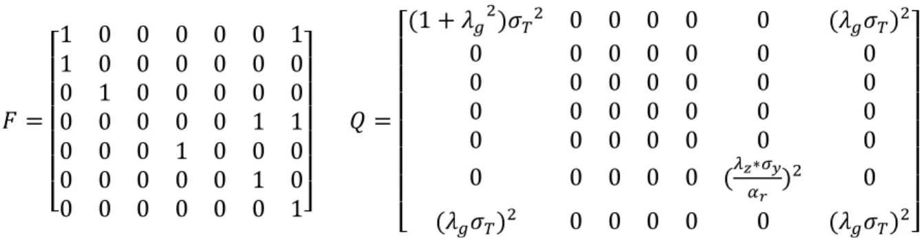
𝐹 =

[

1 0 0 0 0 0 1 1 0 0 0 0 0 0 0 1 0 0 0 0 0 0 0 0 0 0 1 1 0 0 0 1 0 0 0 0 0 0 0 0 1 0 0 0 0 0 0 0 1]

𝑄 =

[

(1 + 𝜆𝑔2)𝜎𝑇2 0 0 0 0 0 (𝜆𝑔𝜎𝑇)2

0 0 0 0 0 0 0 0 0 0 0 0 0 0 0 0 0 0 0 0 0 0 0 0 0 0 0 0 0 0 0 0 0 (𝜆𝑧∗𝜎𝑦

𝛼𝑟 )

2 ₀

(𝜆𝑔𝜎𝑇)2 0 0 0 0 0 (𝜆𝑔𝜎𝑇)2]

The initial conditions for the variable 𝑧_𝑡 were set to zero. For the remaining state variables, the Hodrick-Prescott (HP) filter was applied to the observed counterpart of the series and this

series was used to initialize the state vector. The coefficients were initialized with the

coefficient values obtained from simple OLS regressions using the filtered HP series.

APPENDIX 2 – Tables

Table 1 – Augmented Dickey-Fuller Unit Root Tests, Test Statistics

Variable Italy The Netherlands

Inflation -3.435 * -3.936 **

Real rate -1.421 -1.624

(first-difference) -10.098 ** -5.651 **

Logarithm of real GDP -2.321 -2.116

(first-difference) -5.800 ** -5.650 **

Note: * represents that the null hypothesis of unit roots can be rejected with a 5% level of significance and ** represents that it can be rejected with a 1% level of significance

Table 2 – Parameter Estimates

Parameter Italy The Netherlands

Sample 1980Q1 – 2016Q3 1986Q1 – 2016Q3

𝜆𝑔 0.038 0.038

𝜆𝑧 0.041 0.122

𝛼1+ 𝛼2 0.893 0.973

𝛼𝑟 -0.063 -0.027

(t-stat) (1.970) (0.866)

𝛽𝑦 0.135 0.025

(t-stat) (2.041) (0.657)

𝜎𝑦 0.206 0.237

𝜎𝜋 0.937 0.909

𝜎𝑇 0.615 0.615

𝜎𝑔 0.023 0.023

𝜎𝑧 0.136 1.062

𝜎𝑟= √𝜎𝑔2+ 𝜎𝑧2 0.138 1.062

S.E. (sample average)

𝑟∗ _{1.787 9.342}

𝑔 0.378 0.447

𝑦𝑇 _{1.248 2.678}

S.E. (final observation)

𝑟∗ _{2.437 14.588}

𝑔 0.473 0.633

APPENDIX 3 – Figures

Figure 1 – One-sided vs. Two-sided estimates of the Natural Interest Rate, Italy.

Figure 2 – One-sided vs. Two-sided estimates of the Natural Interest Rate, The Netherlands.

Figure 3 – Real Interest Rate Gap and Output Gap, Italy.

Figure 4 – Real Interest Rate Gap and Output Gap, The Netherlands.

-1 0 1 2 3 4 1 9 8 2 1 9 8 4 1 9 8 6 1 9 8 8 1 9 9 0 1 9 9 2 1 9 9 4 1 9 9 6 1 9 9 8 2 0 0 0 2 0 0 2 2 0 0 4 2 0 0 6 2 0 0 8 2 0 1 0 2 0 1 2 2 0 1 4 2 0 1 6 One-sided Two-sided -10 -5 0 5 10 1 9 8 8 1 9 9 0 1 9 9 2 1 9 9 4 1 9 9 6 1 9 9 8 2 0 0 0 2 0 0 2 2 0 0 4 2 0 0 6 2 0 0 8 2 0 1 0 2 0 1 2 2 0 1 4 2 0 1 6 One-sided Two-sided -10 -5 0 5 10 15 1 9 8 2 1 9 8 4 1 9 8 6 1 9 8 8 1 9 9 0 1 9 9 2 1 9 9 4 1 9 9 6 1 9 9 8 2 0 0 0 2 0 0 2 2 0 0 4 2 0 0 6 2 0 0 8 2 0 1 0 2 0 1 2 2 0 1 4 2 0 1 6

Real Rate Gap Output Gap

-10 -5 0 5 10 1 9 8 8 1 9 9 0 1 9 9 2 1 9 9 4 1 9 9 6 1 9 9 8 2 0 0 0 2 0 0 2 2 0 0 4 2 0 0 6 2 0 0 8 2 0 1 0 2 0 1 2 2 0 1 4 2 0 1 6

Figure 5 – Estimates of the Natural Interest Rate and the Growth Rate of Potential Output, Italy.

Figure 6 – Estimates of the Natural Interest Rate and the Growth Rate of Potential Output, The Netherlands.

Figure 7 – Comparison of the estimates of the Hodrick-Prescott filter and the Kalman filter, Italy.

Figure 8 – Comparison of the estimates of the Natural Interest Rate for Italy and the Netherlands with those estimated by Holston, Laubach and Williams (2016) for the Euro Area.

-1 0 1 2 3 4 1 9 8 2 1 9 8 4 1 9 8 6 1 9 8 8 1 9 9 0 1 9 9 2 1 9 9 4 1 9 9 6 1 9 9 8 2 0 0 0 2 0 0 2 2 0 0 4 2 0 0 6 2 0 0 8 2 0 1 0 2 0 1 2 2 0 1 4 2 0 1 6

Natural Interest Rate Growth Rate of Potential Output

-10 -5 0 5 10 1 9 8 8 1 9 9 0 1 9 9 2 1 9 9 4 1 9 9 6 1 9 9 8 2 0 0 0 2 0 0 2 2 0 0 4 2 0 0 6 2 0 0 8 2 0 1 0 2 0 1 2 2 0 1 4 2 0 1 6

Natural Interest Rate Growth Rate of Potential Output

-4 -2 0 2 4 6 8 10 12 14 1 9 8 2 1 9 8 4 1 9 8 6 1 9 8 8 1 9 9 0 1 9 9 2 1 9 9 4 1 9 9 6 1 9 9 8 2 0 0 0 2 0 0 2 2 0 0 4 2 0 0 6 2 0 0 8 2 0 1 0 2 0 1 2 2 0 1 4 2 0 1 6

Ex-ante Real Interest Rate One-sided Two-sided Hodrick-Prescott

-10 -5 0 5 10 15 1 9 8 2 1 9 8 4 1 9 8 6 1 9 8 8 1 9 9 0 1 9 9 2 1 9 9 4 1 9 9 6 1 9 9 8 2 0 0 0 2 0 0 2 2 0 0 4 2 0 0 6 2 0 0 8 2 0 1 0 2 0 1 2 2 0 1 4