Oil price shocks and the Portuguese economy since the 1970s

(1)

Oil price shocks and the Portuguese

economy since the 1970s

Pedro Brito Robalo

João Cotter Salvado

Abstract:

This paper assesses empirically the effect of oil price shocks on Portuguese aggregate economic activity, industrial production and price level. We take the usual multivariate VAR methodology to investigate the magnitude and stability of this relationship. In doing so, we follow the approach presented in the recent literature and adopt different oil price specifications. We conclude that, as for most industrialized countries, the nature of this relationship changed in the mid-1980s. Furthermore, we show that the main Portuguese macroeconomic variables have become progressively less responsive to oil shocks and the adjustment towards equilibrium has become increasingly faster.

JEL Classification: E32, Q43

(2)

1. Introduction

The relationship between oil prices and the main macroeconomic variables has

been a recurrent research topic since the 1970s. Up to this decade oil prices exhibited a

fairly stable and predictable behaviour. It was not until the oil shocks of 1973-74 and

1979-80 that this variable began to be regarded as a crucial determinant of

macroeconomic stability.

The early studies documented and explained the inverse relationship between an

increase in the oil price and aggregate economic activity. 1 2 A major illustration of the

extent and relevance of this relationship was put forward by Hamilton (1983), who

showed in an influential paper that nine out of ten US recessions since World War II

had been preceded by an oil price increase, i.e. he finds evidence in support of Granger

causality between oil prices and real GNP.

Jones, Leiby and Paik (2003) identify five main branches of research when

assessing the state of knowledge on the impact of oil prices in the economy.

The first is the “mechanisms of effect” topic, which deals primarily with the routes

through which oil prices transmit their effects to the economy at the micro-level. A

plethora of approaches is used when addressing this question: the use of disaggregated

data at the firm level, theoretical models for different market set-ups, etc

A second sub-field addresses the problem of “attribution”, which arose from the

observation that oil shocks were often followed by monetary policy intervention. Some

authors (for example, Hooker (2002)), believe it were not oil price shocks but monetary

policy the main culprit for the stagflation episodes. In a very influential paper,

Bernanke, Gentler and Watson (1997) showed that the Federal Reserve policy is largely

endogenous due to the Fed’s commitment to macroeconomic stabilization. They argue it

is possible that, by reacting to oil price shocks, monetary policy has contributed to

1

Among the early studies, a special mention is due to Pierce and Enzler (1974) and Darby (1982).

2

(3)

deepen stagflation episodes. Such statements lead to a series of replies and

counterfactual studies, launching a debate which has not yet been settled.

A third perspective approaches the stability of the oil price-GDP relationship

over time. Rotemberg and Woodford (1996), among other authors, argue that the nature

of this relationship changed sometime in the 1980s. They justify this change with the

fact that “sometime in the early 1980s, OPEC lost its ability to keep the nominal price

of oil relatively stable. It is reasonable to assume that after this point variations in the

demand for oil … began to be reflected in nominal oil prices immediately”. This claim

poses the following dichotomy: either oil prices ceased to Granger-cause GDP or the

previous linear relationship evolved into a somehow more complex one. One

fundamental question related to this discussion is the empirically observed degree of

asymmetry exhibited by macroeconomic fundamentals in reaction to oil shocks. In other

words, the effects of an increase in the oil price are substantially different from the

effects of a fall in the oil price (see, for example, Mork (1989), who was the first author

to suggest asymmetric specifications for oil price shocks).

The fourth branch is linked to the issue that probably ranks first among

policymakers worries about oil prices: the so-called magnitude of the oil price-GDP

relationship. For the US economy, the empirical tests have produced a negative

relationship as expected.

The fifth and more recent area focuses on the links between oil prices and stock

market performance.

Perhaps not surprisingly, the American economy has been the recipient of the

bulk of empirical studies on the subject. 1 Some authors have extended the analysis to

other industrialized countries (e.g., Cuñado and Pérez de Gracia (2003) for some

European countries, or Jimenez-Rodriguez, and Sanchez (2005) for some OECD

countries). Other authors have studied countries individually (e.g., de Miguel, Manzano,

and Martín-Moreno’s (2003) for Spain and Papapetrou (2001) for Greece). We know of

no detailed or individual study for Portugal.

Our paper’s ultimate purpose is then to investigate the impact of oil price shocks

on the Portuguese economy. An analysis encompassing the entire range of questions

brought up so far would require us to employ multiple methodologies, therefore

implying the risk of losing focus on the main results. Bearing this concern in mind, we

(4)

will restrict our work to the investigation of the magnitude, existence and stability of the

oil price-Portuguese GDP relationship. The estimation of a multivariate VAR fits quite

satisfactorily this goal.

The remainder of the paper is set out as follows. In the next section we present

our methodology and discuss the choice of variables to include in the VAR. In section 3

we run a test on the stability of the oil price-GDP relationship. In section 4 we estimate

the VARs and interpret the magnitude and assess the significance of the relationship

between oil price shocks and our variables. In Section 5 we generate the impulse

response functions and analyse the adjustment towards the equilibrium after an oil

shock. In the last section we present our conclusions.

2. Methodology

We follow the usual vector autoregression (VAR) methodology (see, for

example, Hamilton (1983) or Burbidge and Harrison (1984)) to study the magnitude

effect and the response to impulse function of oil price across the main macroeconomic

variables. 1

The VAR methodology is very useful for this purpose and it is easy to use. A

VAR model can be seen as a reduced form of a simultaneous equations model and, thus,

can be estimated by Ordinary Least Squares, equation to equation.2 These estimations

will be both consistent and asymptotically efficient.

2.1 Choice of variables for the VAR

The variables considered for the model are the following: average oil price

(OIL), real Gross Domestic Product (GDP), Industrial Production Index (IPI), total

employment (TEMP), unemployment rate (UNR) and the CPI-based inflation rate

(INF).

1

Vector autoregression (VAR) is an econometric model used to capture the evolution and the interdependencies between multiple time series, generalizing the univariate AR models. All the variables in a VAR are treated symmetrically by including for each variable an equation explaining its evolution based on its own lags and the lags of all the other variables in the model. Based on this feature, Christopher Sims advocates the use of VAR models as a theory-free method to estimate economic relationships, thus being an alternative to the "incredible identification restrictions" in structural Vector models (Christopher A. Sims, 1980, “Macroeconomics and Reality”)

(5)

The average oil price is the annual average crude oil price converted to the

domestic currency by using the appropriate exchange rate index. The GDP and INF are

included in the VAR since our primary object of concern is the impact of oil prices on

real output and the price level. We include IPI as a measure of industrial production

because we are interested on capturing the effects of oil prices both on industrial

production itself and on GDP through the production capacity usage channel. It is

important to stress that the industrial sector is much more responsive to a change in the

price of oil than, for example, the services sector. The unemployment rate and total

employment are included to clutch not only the direct effects of oil prices on the labour

market but also the effects operating indirectly on output and inflation via labour market

channels. Most studies include monetary policy variables. The reason we leave out such

variables is the fact that, throughout the period covered by this study, the instruments

and the role of monetary policy in Portugal have been neither stable nor clear. We have

taken the logarithm of the first four variables in order to obtain rates of growth with the

first differences. We left the unemployment rate and the inflation rate in percentage

terms.

2.2 Different specifications for oil price shocks

In part due to the volatile behaviour of oil prices, linear oil price specifications

are no longer appropriate if we want to study the true effects of oil price shocks. Hooker

(1996) showed that, for the American economy, (linear specifications of) oil prices

ceased to Granger-cause most macroeconomic indicator variables, including the

unemployment rate, real GDP, aggregate employment, and industrial production. Based

on a paper by Hamilton (1996a), we will define three non-linear proxy variables for oil

price shocks. The first is the evolution of the annual changes of world oil prices and is

calculated as:

) ln( )

ln( − −1

=

∆oil_t oil_t oil_t ,

(6)

Then we specify a variable that considers only price increases. The rationale for

this specification relies on the observed asymmetry in the way the main macroeconomic

variables react to oil price changes:

) , 0

max( _t

t oil

oil = ∆

∆ +

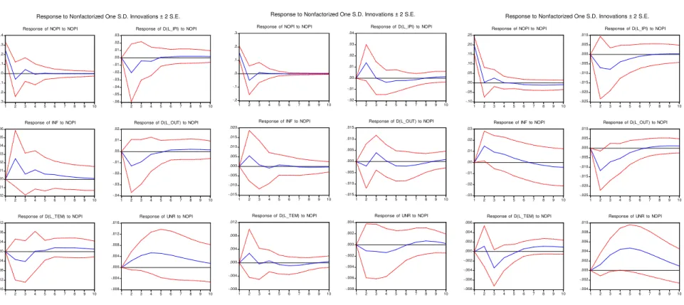
Next we define the Net Oil Price Increase (NOPI). This variable will take into

account an oil price change only if the percentage increase in price is above the

observed values for the previous four years. Otherwise it is zero. This specification

eliminates price increases that simply correct price volatility. This way it captures more

effectively the surprise element, which may be at the origin of a change in spending

decisions by firms and households.In our case, since growth rates are defined as annual

growth rates, we shall calculate:

))] ,

, , ln(max( )

ln( , 0

max[ − ₋₁ ₋₂ ₋₃ ₋₄

= _t _t _t _t _t

t oil oil oil oil oil

NOPI

.0 .1 .2 .3 .4 .5 .6 .7

1970 1975 1980 1985 1990 1995 2000 2005

.0 .1 .2 .3 .4 .5 .6 .7

1970 1975 1980 1985 1990 1995 2000 2005 -1

0 1 2 3 4

1970 1975 1980 1985 1990 1995 2000 2005 -.8 -.6 -.4 -.2 .0 .2 .4 .6 .8

1970 1975 1980 1985 1990 1995 2000 2005

(7)

3. Stability of the oil price-macroeconomy relationship

In this section we want to test whether the nature of the oil price-macroeconomy

relationship changed for the Portuguese case when we assume a linear specification for

oil prices. If this is the case, we must resort to alternative specifications of oil prices. A

good specification for oil prices is the one which successfully represents the oil

price-macroeconomy relationship.

We follow the methodology presented by Hamilton (1983) and perform the

Chow Breakpoint Test on the following equation:

t t t

t t

t

t y y oil oil oil u

y =α+β1 ₋1+β2 ₋2 +β3 +β4 ₋1+β5 ₋2 +

where y is the log of real GDP and oil is the log of average oil prices (note that this is a

linear specification). Any lag length choice can be subject to some kind of criticism. On

a theoretical ground, our choice seems to be balanced.

Several possible breakpoints could be tested. As an illustration, let us mention

that Hooker (1996a) supports the existence of a breakpoint in 1973 and Rotemberg and

Woodford (1996) found a breakpoint in 1980, both for the American economy.

We have chosen not to test for breakpoints in the 1970s due to the risk of obtaining

results with little robustness, given that the first observation in our sample is 1968. We

have tested for a breakpoint on 1985 for two main reasons: there was a clear collapse of

oil prices in 1985-1986 (Saudi Arabia drastically reduced oil prices around this period)

and several authors point to the mid-1980s as the rupture point in the way economic

agents react to oil prices. Both facts can be corroborated by a simple observation of the

series graph. The Chow breakpoint test provides evidence for the existence of a

structural break in this point at the 5% significance level.1

This conclusion has two implications for the remainder of our work. First, we

found more appropriate and insightful to estimate models for different time periods: for

the entire sample, for a first sub-sample (1968-1985) and for a second sub-sample

(1986-2005). Second, we chose to carry out the estimation with the alternative

1

(8)

specifications of oil price shocks presented above. This will allow us to perform a

comparative analysis and conclude if the nature of the relationship has indeed changed.

4. Magnitude and significance of oil price shocks effects

As we are working with annual data we should expect that one lag of the

endogenous variables should be enough to conduct the VAR estimation without

problems. The usual lag length criteria provided support for this choice, so we estimated

VAR Models of order 1. 1

To analyze the effects of the different specifications of oil price changes, we first

studied the coefficients obtained in the VAR estimation and then we performed the

Granger Causality Tests. The VAR estimation produced the coefficients represented in

Table 1.

For the whole sample only the effect to inflation seems to be significant, and this

is verified across all specifications of oil prices. The magnitude of these effects

increases as we pass from oil, to oil+ and from oil+ to NOPI. These variables act

like a filter that transforms variations in the price of oil into shocks and, as a

consequence, it is expectable to obtain greater effects.

Analysing each of the two sub samples separately, we observe that the

coefficients are more significant and that the magnitudes are higher for the first sub

sample.

For inflation we obtain exactly what we made reference to: a higher and more

significant effect for the first sub sample than for the second. The effect on the

unemployment rate, despite not being significant for the whole sample, it becomes

significant for two specifications of oil price variation in the first sub sample.

To analyse the statistical causality link between oil price shocks and the other

variables, we will perform bivariate Granger Causality Tests. The Granger (1969)

approach assesses whether past information on one variable helps in the prediction of

the outcome of some other variable, given past information on the latter.It is important

to note that the statement "x Granger causes y" does not imply that y is the effect or the

result of x. Granger causality measures precedence and information content but does not

by itself indicate causality in the more common use of the term.

(9)

Table 1

INF GDP UNR Temp IPI

oil 0,088* -0,044 0,009* -0,012 -0,063

oil+ 0,077* -0,026 0,007 -0,004 -0,026

NOPI 0,101** 0,053 0,008** -0,013 -0,082

oil 0,032** -0,002 0,006 -0,009 -0,004

oil+ 0,050** -0,004 0,007 -0,003 0,040

NOPI 0,035 -0,013 -0,007 0,018 0,088**

oil 0,055** -0,026 0,006 -0,001 -0,017

oil+ 0,063** -0,039 0,008 0,002 -0,019

NOPI 0,076** -0,061 0,007 0,006 -0,036

First Sub Sample (1968 - 1985)

Second Sub Sample (1986 - 2005)

Entire Sample (1968 - 2005)

Note: INF is the Inflation rate, GDP is the growth rate of Real GDP, UNR is the Unemployment rate, Temp is the growth rate of Total Employment and IPI is the growth rate of Industrial Production Index. One/Two asterisks denote signifance at the 10%/5% level.

We present the p-values associated with this test in Table 2.1

Analysing the results for the whole sample we found Granger causality between

two specifications of oil price and Total Employment, and between NOPI and the

growth rate of GDP. It is important to refer that with this method we do not obtain

significant causality over inflation.

Using only the first sub sample we found causality between all specifications of

oil price and the rate of unemployment, which disappears in the second sub sample.

In the sub sample 1986-2005 we found Granger Causality only between oil and three

variables: GDP growth rate, inflation and total employment growth rate.

1_{It is important to denote that larger}

(10)

Table 2

oil 0,924 0,300 0,096 0,972 0,763

oil+ 0,675 0,447 0,035 0,986 0,732

NOPI 0,613 0,504 0,054 0,966 0,836

oil 0,060 0,067 0,952 0,010 0,570

oil+ 0,378 0,815 0,915 0,573 0,540

NOPI 0,662 0,501 0,874 0,538 0,572

oil 0,324 0,131 0,167 0,025 0,784

oil+ 0,103 0,323 0,236 0,035 0,413

NOPI 0,155 0,085 0,263 0,109 0,326

First Sub Sample (1968 - 1985)

Second Sub Sample (1986 - 2005)

Entire Sample (1968 - 2005)

Note: INF is the Inflation rate, GDP is the growth rate of Real GDP, UNR is the Unemployment rate, Temp is the growth rate of Total Employment and IPI is the growth rate of Industrial Production Index.

We do not observe strong evidence of causality neither for the two sub samples

nor for the entire sample, with the exception of the effect over the unemployment rate in

the first sub sample.

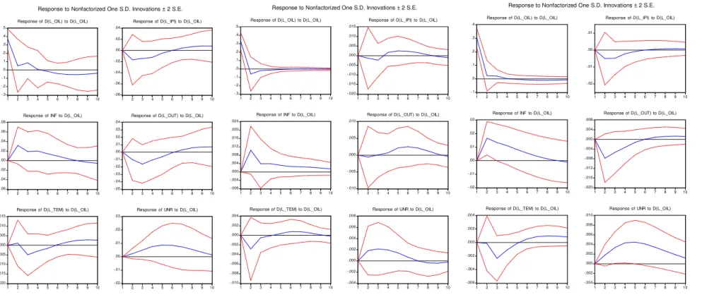
5. Impulse Responses analysis

In this section, we examine the response of each variable of the VAR equations

to a shock in oil price proxy variables. The method that we use is the impulse response

functions. An impulse response function traces the effect of a one-time residual shock to

one of the innovations on current and future values of the endogenous variables.

Therefore it is very useful for the analysis of the adjustment of each macroeconomic

(11)

In the Annex we present all graphical representations of the impulse response

functions that we have generated. By observing them we can conclude some interesting

features; we will organize our findings variable by variable.

The GDP growth rate responds negatively to all oil price shocks specifications

for every sub sample. The initial response is always larger and lasts longer in the first

sub sample for the different specifications of oil price, and changing these specifications

does not change significantly the results.

For Inflation, we obtain always the desired effect: positive responses to positive

shocks. The structure of adjustment after the shocks is very similar across the sub

samples, but the magnitude of the initial impact is bigger for the period 1968-1985.

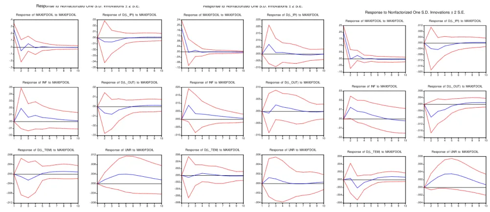
For the Industrial Production Index, even if it is not very large, the initial

response is always negative for the first sub sample and for the whole sample. If we

observe the responses to oil+ and NOPI in the second sub sample, the conclusions are

different: the responses are positive. This may seem a bit confusing; however, it might

simply be related to a weakened relationship between oil prices and industrial

production due to a change in the oil price behaviour.

In what concerns the Unemployment Rate, we obtain the same structure of

adjustment and the expected positive effects for all oil price specifications. The

adjustment is longer in the first sub sample. It is also visible that the Unemployment

Rate is the variable that takes more time do adjust completely.

The effects on the growth rate of Total Employment are similar to the one that

we have observed for the growth rate of GDP. The response is initially negative and the

adjustment occurs faster in the sub sample 1986-2005.

6. Conclusions

In this paper we present a study on the effects of changes in oil price for the

Portuguese economy. We use the VAR methodology, which is commonly employed for

this purpose. We use different specifications for oil price variations and estimate the

effects for different time intervals, namely before and after 1985.

With the VAR coefficient analysis we found a significant effect of variations on

the price of oil over inflation and, only for the first time interval, over the

unemployment rate. The magnitude of the coefficients becomes smaller in the second

(12)

The Granger Causality method allowed us to draw one significant conclusion:

the existence of real causality between oil prices and the unemployment rate in the first

sub sample.

The impulse response functions were extremely useful in analysing the

adjustment and the initial impact of the variations in the price of oil. We found that oil

prices induce persistent effects on unemployment and inflation rates, and not so

persistent effects on total employment and GDP. The response of industrial production

is somehow ambiguous. This approach provided further support for an empirical fact

referred in the literature: generally, after 1985 the effects of oil price shocks become

more tenuous and the adjustment becomes faster.

We found some evidence for the change of the relationship between all

economic variables for Portugal and oil price shocks from the 1980s on. The

significance of the effects, the magnitudes and the velocity of the adjustments are

(13)

Appendix - Data Sources

In this appendix we present the data series we have used, together with the

correspondent source. All series are annual and for Portugal:

GDP: Real GDP in chained 1995 euros; source: Banco de Portugal

INF: Inflation rate, annual Consumer Price Index variation; source: Banco de Portugal

UNR: Unemployment rate; source: Banco de Portugal

Temp: Total Employment; source: Banco de Portugal

IPI: Average of monthly Industrial Production Index; source: Instituto Nacional de

Estatística (Portuguese National Bureau of Statistics)

OIL: Weighted average of crude oil prices; source: Financial Trend Forecaster

ER: Real Exchange Rate Index; source: International Monetary Fund

References

Barsky, Robert and Kilian, Lutz (2004) “Oil and Macroeconomy since the 1970s”,

NBER Working Paper Series, WP 10855

Bernanke, B., Gertler, M. and Watson, M. (1997) “Systematic Monetary Policy and the

Effects of Oil Price Shocks,” Brookings Papers on Economic Activity, 1997(1):91-157.

Brown, S., Yucel, M., (2002) “Energy Prices and Aggregate Economic Activity: An

Interpretative Survey”, The Quarterly Review of Economics and Finance, Vol. 42, No. 2

Burbidge, J., and A. Harrison. (1984) “Testing for the Effects of Oil-Price Rises Using

Vector Autoregression” International Economic Review 25: 459-484.

Cuñado, J., and Pérez de Gracia, F. (2003) “Do Oil Price Shocks Matter? Evidence for

Some European Countries” Energy Economics 25: 137-154.

Darby, M. R. (1982) “The Price of Oil and World Inflation and Recession,” American

(14)

Eastwood, Robert K. (1992) “Macroeconomic Impacts of Energy Shocks” Oxford

Economic Papers, New Series, Vol. 44, No. 3, pp. 403-425.

Finn, Mary G. (2000) “Perfect Competition and the Effects of Energy Price Increases on

Economic Activity” Journal of Money, Credit and Banking, Vol. 32, No. 3, Part 1, pp.

400-416.

Gisser, M., Goodwin, Thomas H. (1986) “Crude Oil and the Macroeconomy: Tests of

Some Popular Notions” Journal of Money, Credit and Banking, Vol. 18, No. 1, pp.

95-103.

Hamilton, James D. (1983) “Oil and the Macroeconomy since World War II” The

Journal of Political Economy, Vol. 91, No. 2, pp. 228-248.

Hamilton, J. D. (1994) Time Series Analysis. Princeton: Princeton University Press.

Hamilton, James D. (2003) “What is an Oil Shock?” Journal of Econometrics, No.

113:2, pp. 363-398 .

Hamilton, James D. (2005) “Oil and the Macroeconomy”, mimeo, prepared for the

Palgrave Dictionary of Economics

Hooker, M. A. (1996a) “What Happened to the Oil Price-Macroeconomy

Relationship?” Journal of Monetary Economics 38: 195-213.

Hooker, M. A. (1996b) “This is What Happened to the Oil Price-Macroeconomy

Relationship: Reply,” Journal of Monetary Economics 38: 221-222.

Hooker, M. A. (2002), “Are Oil Shocks Inflationary? Asymmetric and Nonlinear

Specifications versus Changes in Regime,” Journal of Money, Credit and Banking 34,

pp. 540-561.

Jones, D., Leiby, P., Paik, I. (2003) “Oil Price Shocks and the Macroeconomy: What

(15)

Jimenez-Rodriguez, R., and M. Sanchez (2005), “Oil Price Shocks and Real GDP

Growth: Empirical Evidence for Some OECD Countries,” Applied Economics, 37 (2),

pp. 201-228.

Kilian, Lutz (2005). “Exogenous Oil Supply Shocks: How Big Are They and How

Much Do They Matter for the U.S. Economy?” Working paper, University of Michigan.

Marques, Carlos R. (1998) “Modelos Dinâmicos, Raízes Unitárias e Cointegração”

Edinova

Mork, K. A. (1989), “Oil and the Macroeconomy When Prices Go Up and Down: An

Extension of Hamilton’s Results,” Journal of Political Economy, 91, pp. 740-744.

Mork, K. A., Olsen, Ø. and Mysen, H. T. (1994) “Macroeconomic Responses to Oil

Price Increases and Decreases in Seven OECD Countries,” Energy Journal 15(4):

19-35.

Pierce, J. L., and J. J. Enzler. (1974) “The Effects of External Inflationary Shocks,”

Brookings Papers on Economic Activity 1: 13-61.

Rotemberg, J. J., and Michael Woodford (1996), “Imperfect Competition and the

Effects of Energy Price Increases,” Journal of Money, Credit, and Banking, 28 (part 1),

pp. 549-577.

(16)

-.1 .0 .1 .2 .3 .4

1 2 3 4 5 6 7 8 9 10 Response of D(L_OIL) to D(L_OIL)

-.02 -.01 .00 .01

1 2 3 4 5 6 7 8 9 10 Response of D(L_IPI) to D(L_OIL)

-.02 -.01 .00 .01 .02 .03

1 2 3 4 5 6 7 8 9 10 Response of INF to D(L_OIL)

-.020 -.016 -.012 -.008 -.004 .000 .004 .008

1 2 3 4 5 6 7 8 9 10 Response of D(L_OUT) to D(L_OIL)

-.006 -.004 -.002 .000 .002 .004

1 2 3 4 5 6 7 8 9 10 Response of D(L_TEM) to D(L_OIL)

-.004 -.002 .000 .002 .004 .006 .008 .010

1 2 3 4 5 6 7 8 9 10 Response of UNR to D(L_OIL) Response to Nonfactorized One S.D. Innovations ± 2 S.E.

-.3 -.2 -.1 .0 .1 .2 .3 .4 .5

-.020 -.015 -.010 -.005 .000 .005 .010 .015

-.008 -.004 .000 .004 .008 .012 .016 .020 .024

-.010 -.005 .000 .005 .010

-.010 -.008 -.006 -.004 -.002 .000 .002 .004

-.004 -.002 .000 .002 .004 .006 .008

1 2 3 4 5 6 7 8 9 10 Response of UNR to D(L_OIL)

Response to Nonfactorized One S.D. Innovations ± 2 S.E.

-.3 -.2 -.1 .0 .1 .2 .3 .4 .5

-.08 -.06 -.04 -.02 .00 .02 .04

-.06 -.04 -.02 .00 .02 .04 .06 .08

-.05 -.04 -.03 -.02 -.01 .00 .01 .02 .03 .04

-.020 -.015 -.010 -.005 .000 .005 .010 .015

-.02 -.01 .00 .01 .02 .03

1 2 3 4 5 6 7 8 9 10 Response of UNR to D(L_OIL)

Fig. 2 – Impulse response functions for a one standard deviation innovation in oil

(17)

-.10 -.05 .00 .05 .10 .15 .20 .25

1 2 3 4 5 6 7 8 9 10 Response of MAX0FDOIL to MAX0FDOIL

-.020 -.016 -.012 -.008 -.004 .000 .004 .008 .012

1 2 3 4 5 6 7 8 9 10 Response of D(L_IPI) to MAX0FDOIL

-.02 -.01 .00 .01 .02 .03

1 2 3 4 5 6 7 8 9 10 Response of INF to MAX0FDOIL

-.020 -.016 -.012 -.008 -.004 .000 .004 .008

1 2 3 4 5 6 7 8 9 10 Response of D(L_OUT) to MAX0FDOIL

-.006 -.004 -.002 .000 .002 .004 .006

1 2 3 4 5 6 7 8 9 10 Response of D(L_TEM) to MAX0FDOIL

-.004 -.002 .000 .002 .004 .006 .008

1 2 3 4 5 6 7 8 9 10 Response of UNR to MAX0FDOIL

-.12 -.08 -.04 .00 .04 .08 .12 .16 .20 .24

-.010 -.005 .000 .005 .010 .015 .020 .025

-.010 -.005 .000 .005 .010 .015 .020

-.010 -.005 .000 .005 .010

-.008 -.006 -.004 -.002 .000 .002 .004 .006

-.004 -.002 .000 .002 .004 .006

1 2 3 4 5 6 7 8 9 10 Response of UNR to MAX0FDOIL Response to Nonfactorized One S.D. Innovations ± 2 S.E.

-.3 -.2 -.1 .0 .1 .2 .3 .4

-.05 -.04 -.03 -.02 -.01 .00 .01 .02 .03

-.02 -.01 .00 .01 .02 .03 .04 .05

-.03 -.02 -.01 .00 .01 .02

-.012 -.008 -.004 .000 .004 .008

-.008 -.004 .000 .004 .008 .012

1 2 3 4 5 6 7 8 9 10 Response of UNR to MAX0FDOIL Response to Nonfactorized One S.D. Innovations ± 2 S.E.

Fig. 3 – Impulse response functions for a one standard deviation innovation in oil+

(18)

-.10 -.05 .00 .05 .10 .15 .20 .25

1 2 3 4 5 6 7 8 9 10 Response of NOPI to NOPI

-.025 -.020 -.015 -.010 -.005 .000 .005 .010

1 2 3 4 5 6 7 8 9 10 Response of D(L_IPI) to NOPI

-.03 -.02 -.01 .00 .01 .02 .03

1 2 3 4 5 6 7 8 9 10 Response of INF to NOPI

-.025 -.020 -.015 -.010 -.005 .000 .005 .010

1 2 3 4 5 6 7 8 9 10 Response of D(L_OUT) to NOPI

-.008 -.006 -.004 -.002 .000 .002 .004 .006

1 2 3 4 5 6 7 8 9 10 Response of D(L_TEM) to NOPI

-.004 -.002 .000 .002 .004 .006 .008 .010

1 2 3 4 5 6 7 8 9 10 Response of UNR to NOPI

-.2 -.1 .0 .1 .2 .3

-.02 -.01 .00 .01 .02 .03 .04

-.015 -.010 -.005 .000 .005 .010 .015 .020

-.015 -.010 -.005 .000 .005 .010 .015

-.008 -.004 .000 .004 .008 .012

-.008 -.006 -.004 -.002 .000 .002 .004

-.3 -.2 -.1 .0 .1 .2 .3 .4

-.06 -.05 -.04 -.03 -.02 -.01 .00 .01 .02 .03

-.02 -.01 .00 .01 .02 .03 .04 .05 .06

-.04 -.03 -.02 -.01 .00 .01 .02

-.016 -.012 -.008 -.004 .000 .004 .008 .012

-.008 -.004 .000 .004 .008 .012 .016

Fig. 4 – Impulse response functions for a one standard deviation innovation in NOPI