Oil price shocks and policy implications the emergence of U.S. tight oil production: a case study

(1)

FUNDAÇÃO GETULIO VARGAS

ESCOLA BRASILEIRA DE ADMINISTRAÇÃO PÚBLICA E DE EMPRESAS MESTRADO EXECUTIVO EM GESTÃO EMPRESARIAL

OIL PRICE SHOCKS AND POLICY IMPLICATIONS

, ~ FGV EBAPE

THE EMERGENCE OF U.S. TIGHT OIL PRODUCTION: A CASE STUDY

D ISSERTAÇÃO APRESENTADA À ESCOLA BRASILEIRA DE ADM IN ISTRAÇÃO PÚB LI CA E DE EMPRESAS PARA OBTENÇÃO DO GRAU DE MESTRE

JEFFREY M. VOTH

(2)

JEFFREY M. VOTH

OIL PRICE SHOCKS ANO POLJCY IMPLICA TIONS

THE EMERGENCE OF U.S. TIGHT OIL PRODUCTION: ACASESTUDY

Master's thesis presented to Corporate International Master's program, Escola Brasileira de Administração Pública, Fundação Getulio Vargas, as a requirement for obtaining the title of Master in Business Management.

PROFESSOR ISTV AN KASZNAR, PHD

(3)

Ficha catalográfica elaborada pela Biblioteca Mario Henrique Simonsen/ FGV

Voth, Jeffrey M.

Oil price stocks and policy implications the emergence of U.S. tight oil production: a case study

I

Jeffrey M. Voth.- 2015.

97 f.

Dissertação (mestrado)- Escola Brasileira de Administração Pública e de Empresas, Centro de Formação Acadêmica e Pesquisa.

Orientador: Istvan Kasznar. Inclui bibliografia.

1. Petróleo. 2. Energia. 3. Recursos energéticos. 4. OPEP. S. Organização de Cooperação e Desenvolvimento econômico. I. Kaszna r, Istvan Karoly. II. Escola Brasileira de Administração Pública e de Empresas. Centro de Formação Acadêmica e Pesquisa .. III. Título.

(4)

~ FGV

JEFFREY MICHAEL VOTH

OIL PRICE SHOCKS AND POLICY IMPLICATIONS THE EMERGENCE OF U.S. TIGHT OIL PRODUCTION: A CASE STUDY.

Dissertação apresentada ao Curso de Mestrado Profissional Executivo em Gestão

Empresarial da Escola Brasileira de Administração Pública e de Empresas para

obtenção do grau de Mestre em Administração.

Data da defesa: 26/10/2015.

ASSINATURA DOS MEMBROS DA BANCA EXAMINADORA

;;

I

·~ ,r ~Qr.

L

0-,

~

ao

Karoly Kasznar

Orien1ador (a)

I

(5)

PREAMBLE

"Travei makes one modest. You see what a tiny place you occupy in the world. ·· - Gustave Flaubert (1821 -1880)

Over the past year, there have been a number o f people who h ave helped me order my thoughts and

complete this project. First and foremost, I want to extend my sincere gratitude to my thesis supervisor

Prof. Dr. Istvan Kasznar who- in the best Fundação Getulio Vargas (FGV) tradition- has provided an optimum levei offreedom and guidance. AdditionaiJy, I would like to tank the remaining members ofmy

thesi s committee, Prof. Dr. Fatima Bayma de Bayma from FGV and Prof. Dr. Antonio Carlos Figueiredo

Pinto from Pontifícia Universidade Católica do Rio de Janeiro fo r taking the time to support my defense.

Mil Gracias, Obrigada! I would also like to express my gratitude to the participants from leading think

tank organizations who explicitly asked not to be mentioned by name, but whose insight was a catalyst

for this project. Finally, this thesis would not have been written without the support o f family, friends, classmates, and the incredible faculty at FGV, ESADE, and Georgetown. The program was truly a

rewarding and humbling experience.

(6)

Table o

f

List o

f

Figures

Figure 1. Tight Oi!: A Primer ... ... 2

Figure 2. Tight Oi I Resource Categorizations ... 5

Figure 3. Basic Tight Oi! Supply Chain Process ... ... ... 6

Figure 4. Role ofSupply and Demand ... ... ... ... ... ... ... .... ... .... ... 8

Figure 5. Overview of Survey Research ... ... ... ... 1

Figure 6. SUinmary o f Survey Results ... 2

Figure 7. U.S. Crude Oi! Production ... ... ... ... ... 11

Figure 8. A verage Spot Price ... 12

Figure 9. Consumption: OECD vs non-OECD ... ... ... 13

Figure I O. World Supply vs Consumption ... 20

Figure 11 . Oi! Price Collapse ... 22

(9)

Abstract

How have shocks to supply and demand ajfected global oi! prices; and what are key policy

implications following the resurgence of oi! production in the United States?

Highlights:

The recent collapse in global oil prices was dominated by oversupply.

The future oftight oi! in the United States is vulnerable to obstacles beyond oi! prices.

Opinions on tight oi! from the Top 25 think tank organizations are considered.

Global oi! prices have fallen more than fifty percent since mid-20 14. While price corrections in

the global oil markets resu!ted from multiple factors over the past twelve months, surging tight

oi! production from the United States was a key driver. Tight oi! is considered an unconventional

or transitional oi! source dueto its location in oil-bearing shale instead of conventional oil

reservoirs. These qualities make tight oi! production fundamentally different from regular crude,

posing unique challenges. This case study examines these challenges and explores how shocks to

supply and demand affect global oi! prices while identifying important policy considerations.

Analysis of existing evidence is suppo11ed by expert opinions from more than one hundred

scholars from top-tier think tank organizations. Finally, implications for United States tight oil

production as well as global ramifications of a new low price environment are explored.

Keywords:

Energy; Oil; Economics; Organization ofthe Petroleum Exporting Countries (OPEC);

(10)

1 Introduction

Statting in 2Q20 14, the global oi! market experienced a massive price correction with ptices

declining over 50% to their lowest point before stabilizing in 2Q2015. Preceding this event was a

buildup in the global supply of oil fueled by tight oi! production in the U.S. Tight oil production

nearly doubled total U .S. output o f crude between 2008 and 2015, which greatly reduced the

need for U .S. imp01ts of oil. This freed significant supplies for the global market ata time when

overall demand for oil was slowing on an amlUal basis.

Continued oversupply in 4Q20 14, forced by OPECs decision to maintain production rates and

transfer the role o f "swing producer" to unconventional oi I producers, catalyzed further price

declines. With oi! prices projected to stay within $50-$100 USD through 2025, the future oftight

oil raises many questions as the complex process oftight oi! production is only economical

during periods of high oi! prices.

This case study examines how shocks to supply and demand affect global oi! prices while

identifying important policy consíderations. Analysis of existing evidence from January 2004

through June 2015 is supported by expert opinions from more than one hundred scholars from

top-tier think tank organizations. Finally, implications for United States tight oil production as

well as global ramifications of a new low price environment are explored.

2 Understanding and Defining Key Case Study Topics

2.1 Tight Oil

It was not until the late 1990s and early 2000s that rapid advances in horizontal drilling and

hydraulic fracturing technologíes allowed for commercial production oftight oíl (CBO, 20 14)

(Ladislaw, et al., 2014) (Brown & Yucel, 2013) (Fattouh, 2013). By the mid-2000s, large scale

tight oil production was in place in the U.S., and productíon would rapidly accelerate over the

next decade to elevate the U.S. to be the top global oi! producer in 2014. That same year, the ElA

estimated that tight oil accounted for about 49% oftotal U.S. crude oi! production, up from 2.5%

in 2003 (ElA, April2015).

While the U.S. has seen tight oi! production soar, other countries are now working towards

commercially extracting their own shale resources. Although the technology that allows for tight

(11)

considerations, geology of shale formations, govemment regulations and the price of crude wil l

ali impact the future development of tight oi I in the U.S. and the world (Ashraf & Satapathy,

2012-2013) (Sandrea, March 2014).

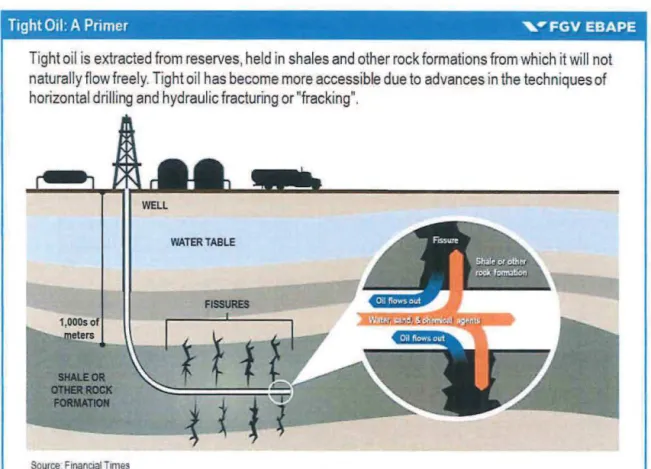
Tight Oil: A Primer ,~ FGV EBAPE

Tight oi I is extracted from reserves, held in shales and other rock formations from which it will not

naturally flow freely. Tight oi i h as become more accessible dueto advances in the techniques of

horizontal drilling and hydraulic fracturing o r "fracking".

Source F1nant~a l Tmes

Figure 1. Tight Oi!: A Primer 2.1.1 The Searcb for a Definition

The geological parameters o f tight oi I differ from those of conventional oi I reservoirs; therefore,

it is considered an "unconventional oil" or "transitional oi!" (Ratner & Tiemann, 20 15) (Pápay,

2014) (Gordon, May 2012). The qualities that make tight oil different from regular crude pose

significant challenges and implications for development. Tight oi I is found in low porous rocks

such as shale, limestone and dolomite about a miJe underground, deep enough such that kerogen

(a solid organic compound that, through retorting, can generate oil) has already been converted

into oil and gas (COGA, 2013). This differs from conventional crude where hydrocarbons

migrate from a source rock to a reservoir rock. The hydrocarbons in shale are locked in place,

(12)

2.1.2 Extraction Techniques

Tight oil extraction requires horizontal drilling, which is more complex than traditional vertical

drilling, and hydraulic fracturing ("frackíng") to release tight oil trapped in low porous rock

(Bommer, 2008). High-pressure water, sand and chemicals are pumped into a well to open

cracks in the rocks, allowing the oi I or gasto be extracted. Shale plays have a high degree of

variation in permeability and required drilling depth, further complicating the extraction process

(Rodgers, April2013). Fracking has come under intense scrutiny for a variety ofreasons,

ranging from the potential of underground water well contamination to allegations of

micro-seismic events (Maugeri, June 2012) (Ratner & Tiemann, 2015) (Schafer, July 2012).

2.1.3 Decline Rates

In addition to the geological characteristics and extraction methods oftight oi!, its production

profiles differ considerably from conventional crude dueto high decline rates. Tight oil wells

peak rapidly during the first weeks of production ("IP30"), register 40-50% lower rates by the

end ofthe first year and decline a further 30-40% by the end ofthe second year. These high

decline rates are charactelistic ofthe industry (Maugeri, 2013) (Sandrea, December 2012).

Conversely, conventional wells display a hyperbolic decline curve that peaks after severa!

months but then stabilizes for periods lasting well over a decade (Rodgers, April 20 13) (Nelson

& Whall, February 2014) (McCracken, 2015). For conventional wells, owners can more readily

recoup the price of drilling the well such that profit can be achieved even during periods of low

oil prices (Tully, 2015). However, tight oi] production requires constant drilling ofnew wells to

generate revenue, thus the value of a tight oil well is short lived (Livingston, 20 14) (Maugeri,

June 2012).

This can be seen in the Bakken oil field, one ofthe largest in the U.S., where the decline rate

over three years is 85% (Hughes, 2014). Additionally, dueto field decline rates ofaround 45% in

the first year alone, larger numbers ofwells are required to increase production figures. For

example, an increase in production of 300 kb/d to 500 kb/d necessitated I ,092 new wells, while

(13)

(Livingston, 2014). With the average cost of each new well at the Bakken of around $7.5 million

in 2014, the need for constant drilling requires significant investment on the parto f producers to

maintain production rates high (KLJ, lnc, 2014).

This can be further quantified by examining ElA Drilling Productivity Reports (DPR) oftwo of

the largest shale plays in the U.S., Bakken and Eagle Ford.1 During the period in which the DPR

has been produced, projected month-on-month new production at the Bakken grew from 86 kb/d

in November 2013 to 92 kb/d in June 2014 (the high mark for oi! prices) and down to 52 kb/d in

July 2015. Legacy declines grew from 60 kb/d to 72kb/d to 74kb/d over the same period (ElA,

October 2013) (ElA, June 2014) (ElA, July 2015). At Eagle Ford, projected month-on-month

new production grew from I 05kb/d in November 2013 to 138kb/d in June 2014 and down to

86kb/d in July 2015. Legacy declines grew from 81 kb/d to 114 kb/d to 141 kb/d o ver the same

period (ElA, October 20 13) (ElA, June 2014) (ElA, July 2015).

Declines in U.S. tight oi! production are primarily caused by the inability of daily production to

keep pace by bringing new wells online. lt is likely that the most productive fields have already

been tapped orare close to depletion, forcing companies to use shale plays that have limiting

factors (Livingston, 2014). Indeed, since May 2015 the sum total ofthe regions that comprise the

DPR have shown production from new wells trailing legacy declines (Nulle, 2015).

2.1.4 Location and Volume

While commercial tight oi! production has so far been primarily confined to the U.S. and Canada

(Argentina began small scale production in 2014), extractable tight oil exists around the world

(ElA, 201 S). lt is estimated that the U.S. has 17% ofthe global total oftechnically recoverable

tight oi! and, as o f l Q20 14, accounted for 91 % o f global tight oi i production with Canada

comprising the remaining 9% (ElA, January 2014). In 4Q20 13, tight oi! production in the U.S.

represented 4.3% of total global crude oil production. The ElA estimates in its projections of

U .S. crud e oi! production to 2025 that ti ght oi! production in the U .S. after 2020 wi ll decline as

production moves into less productive plays (ElA, May 2015) (Blanchard, Spring 2014).

1

(14)

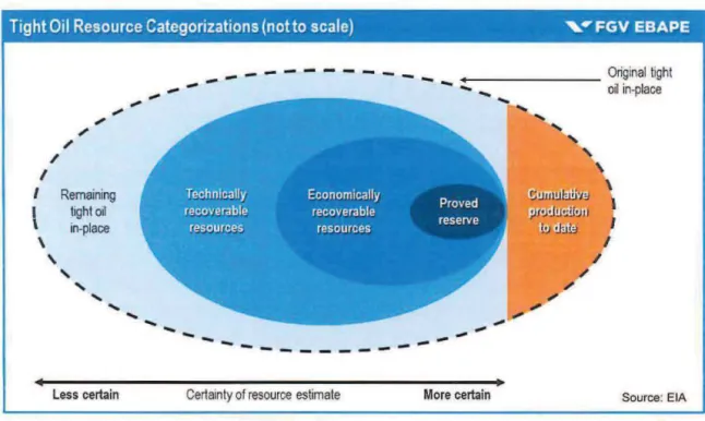
Tight Oi I Resource Categorizations (notto scale) , .. FGV EBAPE

--

_

...

---

Original tight

....

-

oil in-place

....

-....

....

;"

'

/

'

/

'

I

'

I Remaining l C !.l u llJb !i "9~ \

I !lghto11 ;lt~J Í

\ _in-place _~J!lj _~

\ I

'

/

' '

; "

....

_....

_{,_ .!"}

....

-

_....

,.

-

....

---

--

---

-

--Less certain Certainty of resource estimate More certain Source: ElA

Figure 2. Tight Oi! Resource Categorizations

Significant deposits of recoverable shale oi I exist in Russia, China, Argentina and Columbia

(Webster, July 2014) (ElA, June 20 13) (PwC, February 2013). The ElA estimates that

technically recoverable tight oil comprises lO% ofthe world's crude oil, with Russia possessing the largest shale reserves globally (Henderson, October 20 I 3). Exxon Mobil estimates that tight

oil production globally will account for 7% oftotaJ crude production by 2040 (ExxonMobi l,

20 15). Questions remain as to what extent and what impact tight oi! production activities

overseas will have on the industry as there are numerous country specific financiai constraints

and other issues over the recoverability oftight oi! that will pose obstac les to further

development. According to Schlumberger, ooe ofthe world's largest oil field services

companies, non-North American tight oi! production could amount to less than I 0% of global

supply by 2020 though might rise to 50% by 2035 . Argentina, Columbia and Russia could

(15)

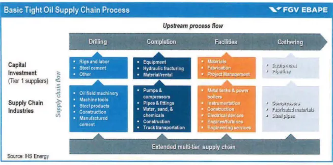
Basic Tight Oi I Supply Chain Process ,..,.. FGV EBAPE

Capital

lnvestment =:

(Ti e r 1 suppliers) ,g

Supply Chaln lndustries

Source HS Energy

;:; ~ ~ Q.. Q. :::> (I)

Upstream process flow

l'lf~-.. .. • ~ ' • . " ,

~ ·· Drilling Complelion Facllilies Gathering

~~

.

• Rigund l1bor • Equopmenl

• st ... l cement • Hydra ulic fracturong

• Othcr • r.latcn allrentrl

• ~~ J ~ I ; .wl~ J J! ~ r l ;J ~IJ. h,

J ~ :JJ I J ;J I :: ~ :n ~

~ i' .l!lrl::-.ilid m ~ !!IJ I.l l ; ~ .:. !J.J~ l;J l;J : ~

~~~ - . .

~:· .. ,_ . . Extended mulli·tier sup~ly chain ••

Figure 3. Basic Tight Oi I Supply Chain Process

2.2 A Primer on Oil Price Economics

Crude oil is a commodity which globally is both greatly abundant and in high demand. The fali

in oi! prices in the second half of 2014 in to 2015 qualifies as a significant event comparable to

two ofthe tive other largest price declines in crude oil over the past 30 years that witnessed 30%

price declines over seven or more months (Baffes, et ai., March 2015). The circumstances

surrounding the price declines in 1985 to 1986 (Oil Glut) and 1997 to 1998 (East Asia financiai

crisis) bear striking similarities to the most recent drop in price. Examining the economics of

crude oi I can give insight into the reasons for oi! price fluctuations and the similarities between

now and the events ofthe mid-1980s and late 1990s.

The price of crude is primarily determined by the basic economic concept of supply and demand

(Energy Charter, 2007; Fattouh, March 2007).2 3 Supply and demand itself can be i.mpacted by a

variety of exogenous market forces, including geopolitical uncertainty, natural disasters and

manipulation by OPEC (The Brattle Group, 2014) (Hamilton, 2009) (NRCAN, October 2010).

2 _{Demand and supply can be captured in a simplc diagram that sums ali the market participants' willingness to buy}

(demand) or scll (supply) at each price. A market is in balance ("equilibrium'') if demand and supply are equal. The price that matches demand and supply is the market price.

3

(16)

Applying the concepts o f short and long run demand and elasticity facilitates a broader

understanding ofwhy oil prices fluctuate.

By August 2015, c rude oil slipped below $40/bbl for the first time since the fallout o f the global

recession, and 50% less than mid-20 14. The last time the oil market experienced such a rapid

price decline was in 2008, a decline brought on by the global recession (Hamilton, Spring 2009).

However, the global economic environment ofthe past year is quite different from that of2008

and, despite uncertain global growth, the IMF forecasts global GDP growth rates of3.4%, 3.3%

and 3.8% in 2014, 20 15 and 2016 respectively, which will result in rising demand for c rude

(IMF, July 2015) (IMF, April2015).

The underlying drivers ofthe 2014 collapse in oil prices are reminiscent ofthe events in 1985

and 1998 (Smith, Summer 2009) (Mabro, 1998) (Hamilton, 2013) (Unalmis, et ai., November

2012). Long tenn supply shifts were the basis for each price fali and, although each event was

unique, sufficient similarities exist to suggest repeated cyclical characteristics. Based on these

events in a market that was characterized by stability for most ofthe 20111 century, it becomes

apparent that the oil market is susceptible to reoccurring "long" or "super" cycles (Cuddington &

Zellou, September 2012).

2.2.1 Role of Supply and Demand

In each event, a decline in demand was the proximate trigger for the price collapse. Between

1984 and 1985, oi! demand growth slowed dueto a global recession brought on by the doubling

ofprices in 1979-80 that forced a general shift away from oil (Helbling, 2013) (Dargay &

Gately, 2010). Between 1997 and 1998, the demand decline was even greater as a result ofthe

East Asia financiai crisis. Most recently, demand has slowed, though not declined, dueto a

gradual reduction in consumption among OECD countries and slower growth in non-OECD

countries. Environmental considerations such as the mild winters in the Northem Hemisphere in

(17)

Role of Supply and Oemand , .. FGV EBAPE

QJ > _Q)

_J

QJ o

-;::

Cl.

p_

Source: G. Mankiw

lonç-nm Aggrega:e Sup:ll'J'

...

-....

-

..

-

...

....

_

Shor~run

Jlçgreg;:e s~p;> J' I

Aggrega!l? Demand .

Aggreg;te Demaod :

Quantity of Real Output

Figure 4. Role of Supply and Demand

More impotiant than demand in t:riggering the price declines was the role of supply and, in each

cycle, a gradual buildup in supply preceded the fali of oil prices. During the 1980s, world oi)

supply actually fel! in 1985 on an annual basis, masking a sharp pickup in the second half ofthe

year that continued into 1986_ In the 1990s, before the peak growth of 1997, supply had been

accelerating over severa! years. Since 201 O, supply growth has been strong with declines only in 2013 (a result of supply inten-uptions brought on by the Arab Spring). The 2000s saw growth

rates in many countries while the massive growth in the

u_s.

can almost be entirely attributed to tight oi i production. Futihermore, in each event, the levei of supply overtook that of demand,

causing a rise of inventaries.

2.2.2 Role o f OPEC

Any discussion of movements in the oi I market would be remiss without mentioning the role of

the Organization ofthe Petroleum Exporting Countries (OPEC) dueto its 40% share of the

market and historical role. Between 1973 and 1988, tbe power to set oil prices was primari1y tbe

reserve of OPEC, though the degree of OPECs influence has decreased in recent years (Fattouh,

January 2011) (Fattouh, March 2007). Today, OPEC can significantly influence crude oil prices

(18)

2.2.2.1 Role ofOPEC: 1984-1985

Despite OPEC reducing its output in an attempt to stabilize prices and justify the 1979-80 price

doubling, crude oi] prices dropped between 1981 and 1985. Saudi Arabia bore the brunt ofthis

policy and greatly increased its output in the second half of 1985, resulting in crude prices

crashing and the 1980s oil glut (Mabro, 1986) (Fattouh & Sen, June 20 15). This move by the

Saudis was aimed at not only recapturing lost market share from non-OPEC producers (primarily

Mexico, the North Sea and Alaska) but also an attempt by Saudi Arabia to restore its market

share within OPEC and impose production discipline on other OPEC members (Gately, 1986)

(Alkhathlan, et ai., 20 14). The resultíng sharp fali in oil prices ended in late 1986 when OPEC

collectively decided to cut back production (Mabro, 2005).

2.2.2.2 Role ofOPEC: 1997-1998

The massive g.rowth of supply in 1997 was driven by increased OPEC output as well as la rge

production increases by non-quota-complying members such as Venezuela (Mabro, 1998). Saudi

Arabia responded by stepping up its own production in the latter half ofthe year as a way to

validate the previous production increases. This production hike was rooted in the misjudgment

that global demand wou1d continue to be high, and there was a s ignificant, concerted quota

increase in N ovember 1997 (Mabro, 1998). By 1998, the East As ia financiai crisis worsened and

oil demand collapsed, resulting in OPEC quota cuts in 1998 and 1999 (PIRINC, August 1999).

However, this action failed to halt declines in oi! prices which continued until mid-1999. In this

case, OPEC was unable to sufficiently cut production to offset oversupply.

2.2.2.3 Role ofOPEC: 2014-2015

In the wake ofthe 2008 financiai crisis, OPEC output rose sharply through 20 12. Dueto

geopolítica! events in OPEC member states such as Libya and Iraq, temporary supply disruptions

occurred in the following years but were quíckly mitigated by expanded output elsewhere

(El-Katirí, et al., March 20 14 ). The decision by Saudi Arabia ( essentially speaking for OPEC) in

November 2014 not to act as swing producer and restrain its production surprised the market and

represented a change in the typical Saudi response to falling oil prices (McNally, October 20 14;

Tortoise Capital Advisors, November 28, 2014) (Fattouh, October 2014). In its effort to maintain

(19)

for market adjustments, OPEC's decision not to cut production despite falling prices forced

immediate further price declines (Deutsche Asset & Wealth Management, November 28, 2014).

2.2.2.4 Role ofOPEC: A Summary

Though the proximate cause differed from case to case, OPEC temporarily relinquished contrai

ofthe market in each ofthese market disrupting events. For each one, corresponding declining

prices resulted from more fundamental economic forces at work distinct from OPEC. Preceding

each major event was a buildup of non-OPEC production driven by a combination of

technological breakthrough and previous high prices that encouraged investment. The power to

contrai the underlying pace of global demand growth is beyond OPEC as it cannot determine

growth in the world economy or changes in energy efficiency. Additionally, OPEC cannot

contrai total supply as it increasingly competes with countries that each act to maximize their

individual supply function (Greiner, May 20 15).

In 1973, OPEC ' s share of global crude production was 51% but dropped to 28% by 1985

(Fattouh, January 20 ll). High oil prices during that time period, brought on partly by OPEC' s

actions, provided the incentive to non-OPEC countries at the time to look for sources of crude

elsewhere and spmTed the development oftechnology to extract it while consumers adapted to

decreased consumption (Morse, 2009). The most recent cycle has similar roots: U.S. exploitation

o f technology to extract tight oi I was made efficient by the high prices o f 2007-14. Significant

production growth in non-OPEC countries, spurred by broader application oftechnology and

reduced production costs, fueled supp!ies (Ratti & Vespignani, 20 15).

2.2.3 Oil Price Cycles

Currently, the global crude market is characterized by dramatic moves in prices and long

fundamental swings in supply likened to the " hog cycle" (Lane, January 13, 20 15). These cycles

occur dueto low supply inelasticity of oil in the short tenn and high elasticity in the long term

(Mankiw, 2007).4 There are two characteristics ofthe oi! market that help dete1mine the supply

response: the capital intensive nature ofproduction and the structure ofthe market.

4 _{Elasticity when discussing oi I prices measures responsiveness of consumption and production o}_f_{oi! to changes in}

(20)

Oil production is typified by a high fixed production cost which then transitions to relatively low

variable production costs.56 Once a field is established, low marginal variable costs of production make it economical and logical for an oil producer to continue to produce even ifprices fali

sharply. ln the long run, supply becomes elastic while production leses efficiency dueto a Iack

o f investment anda failure to put new fields in to production. Historically, production lags take

approximately one year as demonstrated by the sharp falls in production in 1986 and 1999.

Because ofthis lag, inventaries grow as supply exceeds demand for a period after the initial price

fali. The move back to market equilibrium through falling supplies also sees a Jag as producers

need high prices to attract new investment among other considerations.

This cyclical pattem was evident during the 2000s when economic growth in Asia led demand to

greatly exceed supply. Between the East Asia financiai crisis ofthe late 1990s and the 2008

financiai crisis, most commodities saw a double digit annual real price growth (Canuto, June

2014) (Erten & Ocampo, 20 13). Oil alone rose over tenfold between 2004 and 2008. This

supercycle was fueled by growing demand resulting from industrial development and rapid

urbanization in emerging markets and underinvestment in various commodity markets.

In the immediate aftennath o f the 2008 global financiai crisis, all commodities suffered greatly

with oil experiencing a decrease in investment (Hamilton, Spring 2009) (Khan, August 2009).

With a notable exception in the oil sector, most commodities rebounded and peaked in 1Q2011

followed by a steady decline in prices. Slower demand resulting from the recession reduced

investment in supply, though prices would shortly rise above $1 00/bbl as the global economy

recovered in 20 I O and growths in OPEC production in 2011 were limited due to the Arab Spring (Darbouche & Fattouh, September 20 11 ). Faced with hi gh crude prices, there was a sharp

increase in investment particularly in U.S. tight oi! as high prices made it profitable (Fattouh,

2013).

5

http://www .cimaglobal.com/Documents/Student%20docsl20 li _ CBA/C04 _ crudeoil_ march2005.pdf

6

(21)

The structure of the market also has a significant impact on supply. A lthough OPEC does behave

in many ways like a cartel, it does not produce the majority ofthe world ' s crude (Colgan, 20 14).

Many non-OPEC producers are not Iocated in the Middle East andare relatively fi·ee from the

geopolitical events that have negatively impacted that region. Furthennore, while OPEC

members are extremely varied economically, they are somewhat constrained to follow a single

policy. Non-OPEC producers do not face similar constraints regard ing how much they can

produce.

2.2.4 Strength of the U.S. Dollar

A facto r o f oi! prices less mentioned than OPEC but still important is the strength o f the U .S.

do llar (USO). Since the USO is used as the medium of exchange for most global trade, its value

has an impact on prices. When t he USO is weak, oil producers stand to gain; when it is

appreciating, oil producers stand to tose (Obadi, 2012).

3 Oil Price Shocks

3.1 Phase One: Methodology - Questionnaire

A survey on crude oil prices and the impact on U .S. shale oil was conducted to assess the

perceptions and experiences oftop domestic think tank thought leaders. T hese individuais

comprise a diverse group of scholars and active participants on the front !ines ofthe energy,

environmental and economic impact ofthe shale oi! revolution in the U.S. Leading scholars from

the top 25 think tank organizations, as ranked by the Think Tanks and C ivil Societies Program at

The Lauder Jnstitute ofthe Univers ity ofPennsylvania, were invited to participate in the survey

(22)

~

Tlw I audvr ln-.tilllll'

\ \1 t:lrron · • \ n, & ~ i cnu:'

! ·-.n I R\1 11 ll/ 1' 1 ~ ' '" \ \ '-1\

Top 25 U.S Th1nk Tank Survey lssued June 20 15

• Leading Pol~ey , Saence anel

. i\TI.M \ n <.: COLi\CII . Economics Experts

- ·--~--·-

l

A2/

t\'flt u h ii'A mct iL.ln l ~ ..

- C SIS "' ... ,

~

d HQOVER rã' • '""'""""-

STIMSQ N

í i iNST I TUT ION

'fhfo .a

•

HNJI,lfW FôJmr/J IIOII

j

.

COUN CI L.,,

C I' FOREIGN

RELATIONS

\\O IU i t

~ 1 \0 HA II\

1 ~\ 11 " ' li

CARN EGIE COUNCIL

Ctnlto roo

IJ:::J lnterna!ional

VI! Development

~ HAJtV.U.O Kt~tet.cfy 5c.hool f;} B ELFE.R CENTER

HHOOK INCS

M.IER

,.., k te.« ~·l!tttftft~ ,l Alf•lu

c' \ 1:' t- -1 F ' : " ' "''~ t ' ( t'IUt•r ,,...

PcwRcscarch< cmcr

W'f.

1 Wilson ~ Bud"t't .; ~ ' '" .' ' '. , ~. Center ~ lltll ... , l'f.lin

; ~ ~ • 1 " ) ( "\ l'rio titir·-.

• ; " '· \ ) I" M I>A U ... ~1 RIII

',~ , ,. , , ~ l '\..., 1111 fi 1~ \ l lt \IH I (U

•

URBAN o•un1 u ro11n

INSTITUTE

IJTCSP

Respondenl Profile

• 75% Hold a Doclorate

• Faculty from9of tOlhe top U S umvers1ties represenled

107 Responses Analyzed and Catalogued (margin of error 5% ai lhe 95% confidence levei)

Note F1eld survey conducled 1-30 June 2015 uslng Qua1ttcs ll'eb·based tool for creaông and adm1nistering onhne surveys (Georgetown Univers1ty academtc hcense). In order lo ensure htgh quahty of lhe

(23)

The field survey was conducted during the period between the 1st and the 301h ofJune 2015. 170

individuais were invited to participate in the survey. In arder to ensure high quality ofthe

response, only respondents with energy sector expertise in the fields of economics, policy

analysis, and scientific discovery were invited to participate in the survey. During the month o f

June, two separate emails reminders were sent out to encourage pruiicipants to respond to the

survey. At the completion o f the survey the overall response rate was 63% with I 07 respondents.

The margin for eJTor was 5% at the 95% confidence levei.

Ofthe 107 respondents, 75% hold a doctorate, more than halfhold faculty positions at leading

universities, and severa! have help prominent policy positions within the U.S. federal

government, Economists from nine out ofthe 10 leading national universities, according to U.S.

News and World Report, are represented (Princeton, Harvard, Yale, Colombia, Chicago, Duke,

Massachusetts lnstitute ofTechnology, University ofPennsylvania, and Dartmouth) . The

majority of respondents were from the National Bureau of Economic Research (19), RAND

Corporation (15), Brookings Institute (13), Belfer Center at Harvard University's Kennedy

School o f Government (1 0), World Resources lnstiture (9), and the James Baker IIl Institute for

Public Policy at Rice University (6).

The survey asked five questions:

a. The decline in global oi! prices over the past 12 months was primaríly a resulto f ( options).

b. If oil prices stay where they are at today, what impact will there be on U.S. shale oil suppliers?

c. How much more or less capital spending by U.S. shale oil suppliers do you foresee?

d. Do you believe that U.S. shale oi! supply will begin contracting over the next 12 months?

(24)

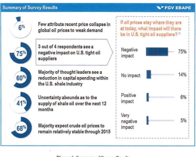
Summary of Survey Results ' .. FGV EBAPE

• .---- -- ---- --- - -- - --- ---

~

: I

f

oil prices stay wher~

they are

:

6%

Few attribute recent price collapse in _{global oi I prices to weak demand} at today, what impact wi ll there

____./ be in U.S. tight oi I suppliers? 11

I

~

3 out of 4 respondents see a

negative impact on U.S. tight oi I Negative

75% :

suppliers impact

I

:~

Majority of thought leaders see a

I

reduction in capital spending within No impact

14% :

the U.S. shale industry

4~

Uncertainty abounds as to the Positive

I

6%

supply of shale oi I o ver the next 12 impact

months

-

Very

.a

negative

I

5%

Majority expect c rude oil prices to _impact

remain relatively stable through 2015

I

L

-Figure 6. Summary ofSurvey Results

3.1.1 Few Attribute Colla pse in Oil P rices to Weak Demand

Few attribute the recent price collapse in global oi/ prices to weak demand

Whi le 42% attributed the price correction to an equal balance of oversupply and weak demand,

the difference between those who pointed to e ither supply or demand was wide. A total of 40%

cited oversupply wh ile only 6% responded that weak demand was the primary cause. Out ofthe

total respondents, 82% and 48% recogn ize the signifi cant impact of oversupply and weak

demand respectively.

3.1.2 Negative Impact on U.S. Tight Oil Suppliers

(25)

At 75%, the overwhelming majority ofrespondents believe that current low oil prices will

negatively impact shale oil producers in the U.S. Additionally, more respondents believe that

there will be no impact than those who believe the impact will be positive, very positive, or very

negative. Overall, 80% see a negative impact, and only 6% project a positive impact. These

assessments are reflective ofthe general opinion ofthe oi! and financiai industry. When the

survey was conducted, the selling price ofWTI was below the breakeven price for a significant

number of shale producers. Even for those who are operating profitably, the reduced net profit

will negatively impact future operations.

3.1.3 Reductions in Capital Spending

Majority oj thought leaders se e a reduction in capital spending within the U.S. Shale industry

Nearly half ofthe respondents (45%) believe that CAPEX spending will decline slightly over the

next 12 months while an additional 15% envision more significant declines. Conversely, 14%

project see a slight uptick in spending while only I% believes much more spending will occur. In

t he middle are the 25% who predict that overall CAPEX spending will remain roughly the same.

Regardless, those who envision reduced spending outnumber those who envision spending

growth by 4:1. CAPEX declines are already being seen in large scale Jayoffs, reduced

exploration o f plays, cancelation o f future projects and consolidation o f existing operations.

3.1.4 Uncertainty Abounds Over Tight Oil Supply

Uncertainty abounds as to lhe supply o

f

shale oil over the next 12 months

While 41% ofrespondents do not envision a contraction ofU.S. sha\e oil over the next 12

months, 27% are unsure while 32% envision declines. Although the forecast of a positive future

for the shale industry received the highest response, the fact that the majority responded with

uncetiainty or negative predictions is significant. Even so, a high number predicts supplies

remaining stable, and this Jogically points to the lag that exists in the market. Despite the

declining prices in 1 Q20 15, production at shale plays ( oil-bearing shale formations) remained

stable as producers were protected by long tenn hedges and newly dug wells being brought

(26)

3.1.5 Think Tanli Leaders See Prices Stabilizing

Majority expect crude oi! prices to remain relatively stable through 2015

The overwhelming majority ofrespondents (68%) envision a closing price of$60-$80/bbl by the

end o f the year. While 15% see a price range o f $40-$60, 13% predict prices o f $80-$100. Only

4% envis ion prices outside ofthe $40 to $ 100 range. Overall, oi! prices are projected to rise by

the end o f the year but w ill not match their highs o f 2014. This price range matches ElA

estimates and, though the range is wide, points to rising but manageable prices.

3.1.6 Hypothesis Testing- Analyzing Questionnaire Data

Three hypotheses about the data were tested. "Don't know" responses were treated as missing

data and were not included in the non-parametric tests described below. Throughout the

analysis, the ability to perfonn statistical tests on the data obtained was intentionally limited

based on the non-parametric data available. Data obtained from respondents was either

categorical or ordinal, with only a few response options possible for each question. From t he

onset, this eliminated severa! types of data analysis such as regression and t-tests which is why

Chi-square and Kruskal-Wallis tests were run using IBM SPSS version 22. Two independent

variables, the respondents' institution and highest leve! of education, could have tested the

difference in response applying an analysis ofvariance (ANOVA), however the descriptive data

was determined to be sufficient to show the consensus among respondents.

3.1.6.1 Hypothesis l(a) and l(b)

Respondents who believed that the decline in oil prices over the past 12 months was a result of

excess supply would predict (a) less capital spending over the next 12 months by shale oi!

suppli ers and (b) shale oil suppliers will begin contracting over the next 12 months.

For hypothesis la, a Kruskal-Wallis test, which is a method for determining ifmultiple samples

come from the same sample, did not reveal any significant differences between belief in the

causes o f o i! prices and prediction of capital spending over the next 12 months by shale oils

suppliers. This is primarily beca use approximately equal groups of respondents chose "excess

(27)

predictions about capital spending by shale oil suppliers. Both groups predicted Iess spending in

the next 12 months by shale oil suppliers, with the majority ofboth groups predicting " somewhat

less spending" and some predicting "much less spending."

For hypothesis 1 b, a Chi-square test, which is a method for determining the similarity between

observed data and projected data, did not reveal any significant differences between belief in the

cause ofthe decline in oil prices and prediction ofwhether shale oil suppliers would begin

contracting in the next 12 months. Again, this is primarily because approximately equal groups

of respondents chose "excess supply" and "equal parts excess supply and weak demand," and

those two groups made similar predictions about whether shale oil suppliers would begin

contracting in the next 12 months.ln both groups, a slight majority predicted that shale oi!

suppliers would not begin contracting in the next 12 months.

3.1.6.2 Hypotbesis 2

Respondents who forecasted less capital spending by U.S. shale oil suppliers would also predict

a reduction in supp1y, or that shale oil suppliers would begin contracting in the next 12 months.

A Kruskal-Wallis test, which again is a method for determining ifmultiple samples come from

the same sample, revealed a significant difference (X2

=

4.57, df=

l,p

=

.033) between

predicting that U.S. shale oi! suppliers would or would not begin contracting in the next 12

months, based on the respondents' forecast of capital spending by U.S. sha1e oil suppliers.

Respondents who forecasted less spending predicted that U.S. shale oil suppliers would begin

contracting in the next 12 months.

3.1.6.3 Hypothesis 3

Respondents who predicted that crude oi! prices will remain stable would also predict a negative

impact on U .S. shale oi! suppliers.

The survey data were not sufficient to test this hypothesis because of lack ofvariability. Most

respondents predicted stable oi I prices and negative impact on shale oi!, and there were too few

(28)

3.1.7 Summary ofResults

Responses to the survey, supported by trends wíthin the industry, forecast that sustaíned low o i i

prices will negatively impact the U.S. shale industty. Substantially reduced profit margins will

prevent substantial growth and expansion in an industry that requires constant capital. By the end

ofthe year, oi! príces are not expected to rise significantly. However, prices at the upper limit

may allow many U .S. shale producers to achieve net profit. Despite the uncertainties, limited volatility is projected for the supply of shale over the next 12 months as shale producers w ill

continue to operate until they are forced to shut wells.

3.2 Phase Two: Explanatory Research

3.2.1 A Decade ofVolatility: 2004-2013

In the decade between 2004 and 2013, an incredible degree of change occurred in the global

crude market. Rising global demand for crude in the wake ofthe late 1990s East Asia financiai

crisis could not be met immediately by matching increases in supply, res ulting in crude oi! prices

reaching a historie high before the recession of 2008 forced prices downward. To cope with the

higher prices, unconventional sources of oil were tapped, and this would play a major role in

shaping the price correction and decline o f 2014 which continued in to 2015.

The second half ofthe 2000s would see tremendous growth in the production ofunconventional

oils paiiicularly in the U.S. High oi! prices spurred the development ofnon-OPEC based energy

resources while changes in consumption, consumer trends and govemment mandates minimized

the need for OPEC sourced oi!. The result was the U.S. shale oi! boom that allowed for the U.S.

to reach its highest crude oil production leveis in four decades (Jr. & Tom, 20 15). In the Bakken

alone, production increased from a few barreis in 2006 to over 530 kb/d in December 201 1 to

over 1 mb/d in December 2014 (ElA, December 2014). This is an amount equal to cun·ent

production leveis ofthe sixth largest oi! exporter, Iraq (Ladislaw, et al., 2014, p. v).

A number o f factors contributed to this rise in oi! prices and parallel development o f tight oi! (Fattouh, January 2010). One ofthese was the earlier mentioned commodity supercycle that

occurred in the wake o f the East As ia financia] crisis, fueled by growing demand ín emerging

markets and underinvestment in various commodity markets (Canuto, June 2014) (Erten &

(29)

While world demand increased, global supply failed to keep pace owing to global instability and

limits on traditional crude production (Livingston, 2014, p. 31). For the first time since oil

drilling began in the mid-191h century, crude prices increased for seven consecutive years from

2002 to 2008. This catalyzed the beginning ofthe U.S. tight oil boom that began in eamest in

2008 (Gordon, May 2012).

3.2.1.1 Increasing Global Demand

The 2000s saw a global shift in the demand of oil. OECD countries, once the biggest consumers,

were supplanted by rapidly developing countries such as China and India whose growth led to

strong increases in demand that offset declines elsewhere in the world (Baffes, April 9, 2012)

(Finley, 2012).7 Between 2000 and 2010, consumption in OECD countries declined while non-OECD consumption rose by 40% with the period between 4Q2005 and 2Q2010 seeing almost

constant declines in consumption by OECD countries (ElA, 20 15). Furthennore, consumption

overall among non-OECD countries only declined in two quarters between 1Q2001 and 2Q20 15

(ElA, 2015). As early as 2006, demand from non-OECD countries had essentially eliminated the

world's spare crude production capacity (The Brattle Group, 2014). Increased demand from

non-OECD countries and decreased global supply resulted in a tightening world market for oil and

increasing prices until 2008.

Demand in developing countries is especially visible in China's and Jndia's massive industrial

development and rapid urbanization. China's share ofworld consumption was 12% in 2014, up

from 8% in 2004 (BP, June 20 15). Although economic growth is slowing in China, increasing

annual consumption in that country is a long term trend (The World Bank, June 20 15). The ElA

has reported that China and lndia will be responsible for half ofthe increase in the world's

consumption of energy between 2008 and 2035 (ElA, September 2014).

7

(30)

Between 2004 and 20 14, demand generally rose at a steady rate but did ta per off in the

immediate aftermath ofthe global recession in 2008-2009. In 2008, the global financiai cri sis

caused annual worldwide oi! consumption to decline for the first time since 1993. As demand

collapsed, oil fell from its ali-time high of $1 44.22/bbl for Brent on July 3, 2008 to a low o f

$33.50/bbl by December 23, 2008, a 77% decline (BP, June 2009). This was especially apparent

in advanced economies like the U.S. and Japan where the decline in oi! consumption more than

offset the consumption growth experienced in some other regions (IMF, October 2009)

(Yanagisawa, March 20 I 5). 8

Economic recovery in 201 O would increase demand and by early 20 I I the price of oi! had once again passed $ 1 00/bbl. However, increasing demand was not compensated by increasing global

oi! supplies dueto a variety offactors. In the U.S. alone, between 2013 and 2014 demand was

relatively stagnant (ElA, July 2015). Govemment mandated fuel economy for cars, ethanol

replacing a portion of oi! used in gasoline, substitution of oi! demand by shale derived gas/NGLs

and the slow and uneven economic recovery ali contributed to reduced demand for crude oi!

(Troner, October 2014). Since 2007, impo1ts ofcrude oi! into the U.S. have steadily declined due

to rising domestic supply from tight oi i and falling consumer demand (ElA, 20 15). In 2005,

imp01ts into the U.S. from outside North America were around 9mb/d but would fall to

approximately 1.95mb/d by mid-2014 (Livingston, 2014).

3.2.1.2 Stagnant Global Supply

As global demand rose from 2005, global conventional crude oil production went into decline as

exports fell from their peak that same year, resulting in crude oi! prices sharply rising in both

nominal and real tenns. Between 2005 and 2008, stagnant oil production and accelerating

demand, particularly from China, fueled oil prices to hit an ali-time high in July 2008.

8

The steep decline in oil prices in the wake o f the fi nanciai crisis was due primarily to common factors and quickly rebounded. These common factors included the sudden drop in demand due to the financiai crisis, global

(31)

Compounding limited growth in oi! production capacity in the first half ofthe 2000s was

instability and conflict in the MENA region that would last throughout the decade. In the Jatter

half o f the 2000s, this caused reductions in supply and led to fears o f future geopolitically

induced production cuts (Amenc, et ai., November 2008) (Darbouche & Fattouh, September

2011). Production disruptions in lraq and Venezuela in the early 2000s were offset by increased

production from other OPEC countries, especially Saudi Arabia. In compensating for these,

OPEC decreased its spare production capacity which Iimited its ability to meet rising demands

and act as a traditional swing producer (Fattouh, October 2014) (Hamilton, 20 I 3 ). Spare capacity

in OPEC increased only marginally between 3Q2005 and 2Q2007 by 1.3mb/d which was not

enough to offset increasing global demand (Murphy, April 14 201 I) (ElA, 2015).

Between 2005 and 2008, net increases from non-OPEC producers were small, and annual growth

averaged 200kb/d (ElA, 20 15) (EJA, February 2008). Majority growth in overall global oi!

supplies since 2005 resulted from the production ofunconventional oils such as tight oi! outside

ofOPEC.lndeed, between 2000 and 2013 crude oil production increased daily by 7.4mb/d

though the majority ofthat, 71% or 5.2mb/d, occurred between 2000 and 2005. The period

between 2006 and 2013 only accounted for 29% or 2.2mb/d ofthe increase. Without the surge in

tight oi! from the U.S. in 2008, total crude production globally wou1d have been in decline with

little to no spare capacity (Fattough & Sen, September 2013) (Maugeri, 2013).

This relatively small increase in conventional global crude output between 2005 and 2008 is

contrasted by increasing prices. This imbalance is attributable to a lack of high spare capacíty

among producers. Accelerating decline rates in ageing conventional fields and a shortage of

easy, cheap alternative sources of conventional crude can partly explain for the absence of

significant expansion in cru de output (SmTell, et al., 201 0).

Piior to the 2008 financiai crisis, OPEC countries were persuaded in 2007 at Jakarta to increase

production for the first time in two years. This was despite early signs of economic instability

coming from the U.S. in the forro ofthe subprime mortgage crisis, and the economic crisis in the

following year would lead to an immediate reversal of OPEC' s decision to increase production

(32)

production in the second half of2008 and in 2009. OPEC would increase supply again in 201 O as demand rebounded, and by early 2011 c rude had passed $1 00/bbl. Even so, OPEC production

cuts were not fully reversed unti1 2012 (BP, June 201 O) (BP, June 201 1).

In the 2010-2012 period, economic recovety led by East Asia res ulted in increased demand.

However, demand exceeded supply, and this was compounded by other factors leading to

increasing prices. Supply disruptions resulting from the Arab Spring impacted operations in

Libya and elsewhere, economic sanctions imposed against Iran for its nuclear program

substantially reduced supplies and non-OPEC areas such as the North Sea and Mexico witnessed

declines in production (Azzarello & Wightman, July 7, 2014) (Stevens, March 2015) (EI-Katiri,

et ai., March 2014). Adding to this was the impact of speculation and fears offurther negative

events on the future trading markets (Amenc, et ai., November 2008). These factors led to high

oi! prices in world markets though notas high as those of2008.

Oi! prices would not stabilize again until 2011 when they reached leveis aligned with or close to

average ali-time highs. This stability was brought about by a solid balance between supply and

demand as well as other factors. Again, the impact of supply disruptions had negative

repercussions on the levei ofworldwide spare oi! production capacity between 2012 and 2013. In

20

t

I alone, Libyan oi! production dropped over I mb/d, forcing increased production elsewhere

(ERGO, February 2012). Declines in OPEC spare production capacity continually dropped until

reaching a low o f 1.6mb/d in 3Q20 13, a situation reminiscent o f the mid-2000s (ElA, 20 15).

3.2.1.3 Surging

U.S.

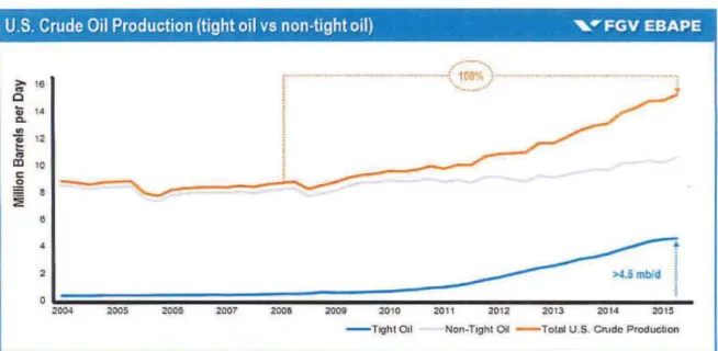
Unconventional Resources

U.S. production ofcrude fueled by tight oil grew by nearly 100% between 2008 and 2015 as the

largest tight oil fields in the U.S. (Eagle Ford, Bakken and Permian) increased production from

less than 0.4mb/d in 2007 to over 3 .5mb/d at the beginning of20 15 (Baffes, et ai., March 20 15)

(ElA, 2015) (ElA, January 201 5) (Fattouh, October 2014). Tight oil production in the U.S. has

been credited with reversing the slump the U.S. has experienced in crude production since its 1ast

peak in 1970 (IMF, 2011 ). From a negative annual growth in crude production in 2008, 1 mb/d o f

oil was added in 2011 and 2012 before rising even higher in the following years (Fattough &

(33)

U.S. C rude Oi I Production (tight oi I vs non-tight oi I) , .. FGV EBAPE

~ 16

o

Ui 14

o.

"'

~ 12

(;

fD 10

c o

§ 8

~

e

4

2

...

!

I

,...

--- · --- --- --- --- --- ---' 100 \ _

' ...

0 ~~~~~~~~

2004 2005 2005 2007 2008 2009 2010 2011

~--~--~

2012 20 13 20 14 20 15

- ToghtOII Non-T1ght 01t - Total U .S. Crudo Produc~on

Figure 7. U.S. Crude Oil Production

3.2.2 Oil Prices Collapse: 2014-2015

In 3Q2014, oi I prices would begin a steep decline from almost $116 on June 17, 2014 that would

continue into 2015 with the price of Brent tluctuating between $47 and $57 from its 1owest point

through the start of2Q20 15.9 This nearly 60% decline was brought about by a number offactors though oversupply is widely accepted to have been the dominant cause in triggering and

motivating the June price correction (Badel & McGillicuddy, 20 15) (Baffes, et ai., March 20 15)

(ExxonMobi1, 20 15) (Nulle, 20 15) (Thomson Reuters, February 2015) (Arezki & Blanchard, December 22, 2014) (Hamilton, December 14, 20 14). Throughout the price correction, supp1y

has continuous1y exceeded demand, but demand factors have increasingly come into play ( Kirby

& Meaning, 20 15).

9

(34)

Average Spot Price (January 2004- June 2015) , ... FGV EBAPE

õi 120 :::

"'

ID

~

.,

100

a. ;;;

.· -~ ~: - ') o so

(.)

ç

so

40

20

- wes~ TeJ<aS1n11!lmOdl010 Cruee Ot Prlce

2005 2006 2007 2008 2009 2010 201 2 4013 2014 2015

Figure 8. A verage Spot Price

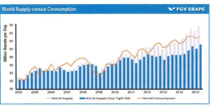
3.2.2.1 Supply and Demand

According to the IEA, global demand slowed from 9 1.9mb/d in 2013 to 92.6mb/d in 2014 while

supply increased from 91.3mb/dto 93.7mb/d, creating an oversupply of 1.4mb/d. In 1Q2015, the

difference was even more pronounced with a 1.8mb/d oversupply (JEA, July I O, 20 15).

3.2.2.2 Demand

Global growth has continuously failed to meet forecasts, and this has serious ly impacted

demand. ln July 2014, the ElA, IEA and OPEC forecasted 2015 globalliqu ids growth to be 1.7

on average. However, by December 2014 the forecast was revised down to 1.1% (Deloitte,

20 15). Ln OECD countries, declining consumption that began in the 2000s continued partly due

to increasing gas efficiencies worldwide and changing consumer trends (ElA, 20 15). Adding to

this were continued economic fears in Europe over issues in countries such as Greece, leading oi i

demand in Europe to sink to its lowest in over 20 years (BP, June 20 15).

Government legislation in the U.S. leading up to 2014, such as the 2005 Energy Policy Act and

the 2007 Energy Independence Act that outlined higher fuel economy standards for vehicles and

(35)

over 2mb/d between 2005 and 20 13. Similar legislation has been enacted elsewhere in OECD

countries and contributes to dec)jning demand (Thomson Reuters, February 20 I 5).

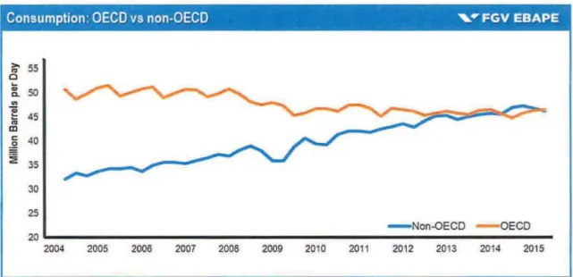
In 2014, China's slowing economic growth, which had been the largest single source of

increasing crude demand, served to limit growth of oil consumption growth (The World Bank,

June 20 15) (ElA, May 20 15) (The Economist, 20 15). That year, the Chinese economy grew by 7.4%, a healthy amount though a decline from the average annual growth rate of I 0% that had held steady for three decades (IMF, April2015). For non-OECD countries, while demand

remained positive, annual growth had slowed considerably with 1Q2013 being the last time

demand growth exceeded 4% over the previous quarter (ElA, 20 I 5).

Consumption : OECD vs non-OECD ,.,. FGV EBAPE

>- ₅₅

"

o

_...

., 50

c..

.,

~ <V 45

m

r:: ₄₀

~

~ ₃₅

30

25

- Non-OECD - OECD

20

2004 2005 2006 2007 2008 2009 2010 2011 2012 2013 2014 2015

Figure 9. Consumption: OECD vs non-OECD 3.2.2.3 Supply

OPEC Supply Changes

In the preceding decade, OPEC saw its share ofthe global crude market gradually erode due to

rising tight oil production in the U.S. and its own price targeting range. To reverse this, severa!

OPEC members, including Saudi Arabia, began in 3Q2014 to export crude to East Asia at

(36)

falling prices, OPEC production increased in September, the largest increase in almost three

years (Smith, 2014).

In Vienna on November 27, 2014, OPEC decided against cutting production as a way of

stabilizing prices and instead agreed to maintain the existing 30mb/d production levei (OPEC,

November 27, 2014) (El Gama!, et ai., 2014). Saudi Oil Minister Ali ai-Naimi stated the move

was an attempt by Saudi Arabia, the world' s largest Iow cost producer, to retain market share and

fend offnon-OPEC competitors (ThomsonReuters, 2015).

lmmediately, Brent fell over $6 on that day alone, a 5% drop to $72.82 (BBCNews, 2014). Over

the com·se ofthe next month, Brent would continue to fali to $59. This decision by OPEC

benefitted the Gulf state members but was opposed by others such as Venezuela, Algeria and

Iran who sought production cuts as falling prices seriously impacted their revenue streams.

The agreement by OPEC was a rejection of its past objective to target an oi! price band and the

start of a new objective to maintain market share. Before this, OPEC had acted as a swing

producer, but that role would now fali on other oil producers such as those in the unconventional

field. Despi te an oi! price plunge of 40% since the previous year, in June 2015 OPEC ministers

refused to cut production, signaling intent to maintain production rates that were actually

marginally rising (Faucon, et ai., 2015) (OPEC, June 11, 2014).

Non-OPEC Supply Changes

In the U.S., total crude production throughout 2014 and into 2015 was nearly double what it was

in 2008, primarily dueto tight oi! production which the IEA considers to be the single largest

source ofincreasing crude supply globally (IEA, 2015). U.S. production between 2008 and June

2014 rose from 5mb/dto 8.5mb/d, a 71% increase. Even as oi1 prices fel! in the latter half of

2014, U.S. oi! production continued rising from an average of8.5mb/d in 2014 to 9.7mb/d by the

stmt of2Q2015 (ElA, 2015). Overall, the 4.7mb/d rise in U.S. production between 2008 into

2015 represents almost 15% oftotal OPEC output in May 2015 (IEA, July 10, 2015). This

increased production reduced U.S. need for imports and freed up millions ofbarrels a day for the

(37)

Despite the negative economic impact falling prices had on tight oi! producers in the short run

going into 2Q2015, the effects were not nearly as bad as had been anticipated (The Economist,

20 15). Due to a backlog o f wells and price hedges sheltering tight oil producers from the

downtum, U .S. supply continued to increase in 2015 even as overall production fell (BlackRock,

Februaty 2015) (ElA, July 2015). The ElA estimates U.S. crude production for 2015 rose by

200/kbd (ElA, July 2015).

Apart from the U.S. and tight oil, there were also production increases in Canada and Brazil as

well as from other unconventional sources. Led by the U.S. and Brazil, biofuel production in

2014 produced almost 1.4mb/d c rude equivalent in 2014 with the top two countries responsible

for 68% of global production. Extraction of oi! from oi! sands in Canada produced 4mb/d of oi!

in 2014.

3.2.2.4 Geopolítica! Challenges

Playing into supply were geopolítica! concerns and events. In 2014, global geopolitical tensions

abounded, including the conflíct in East Ukraine, the ISIS offensives in Iraq and sectarian

violence as well as the !ack of a stable government in Libya. Despite these crises, which would

give commodities traders reason for caution and speculation over supply disruptions ultimately

leading to higher prices, quite the opposite occuned (ai Harmi, 2014). Preliminary fears over

potential supply disruptions in 20 14 proved mostly unfounded.

lSIS, which has been on the offensive in Jraq since late 2013, went on to capture Mosu1, lraq's

second largest city, in June 2014 before their offensive stalled out (Nordland & Rubin, 2014). Fears of large sca1e cuts in overalllraqi oi! output dueto the loss of northern oilfields were also

unfounded as production increased rapidly in the south and in Kurdistan (Co1umbia SIPA, 2014)

(Edinburgh International, 20 14). lnstead of declines, lraqi output actually increased in 2014 with

an output average o f 330kb/d over 2013 and was the second leading contributor to global oi!

(38)

Meanwhile in post-Gaddafi Libya, production which had fallen by over 80% from its highs in

I Q20 13 to its lows in 2Q20 14 saw production gradually increase fourfold by the start o f 4Q20 14

before falling again (Faucon, 2014) (Trading Economics, 2015). Despite the p!acement of

economic sanctions on Russia as a result ofthe conflict in East Ukraine, declines on the total

output from Russia were short lived and mínima! with production immediately increasing in

3Q2014 and eventually hitting its highest output over the past decade by 1 Q2015 (Trading

Economics, 20 15) (Morgan, 20 15).

3.2.2.5 Appreciation ofUS. Dollar

Beginning in the second half o f 2014, the USD began a rapid appreciation against other major

currencies, totaling over 20% between 2Q2014 and 2Q2015 (ODI, March 2015). As stated

earlier, since most commodities including crude are traded in USD, a rise in the value ofthe

do !lar tends to negatively impact oil producers while decreasing demand by reducing the

purchasing power o f other countries (Deloitte, 20 15). Monetary policies in the U .S. h ave played

a considerable role in the appreciation ofthe USD (Frankel, December 2014).

Overall, the significant but not unprecedented price decline between 2014 and 2015 was

dominated by an excess of supply resulting in a price correction. While supply was the primary

driver, the impact of slowing demand is significant. Revised forecasts and estimates continue to

show that demand has been repeatedly less than originally anticipated. Furthennore, the

appreciation ofthe USD and the failure of supply disruptions to have meaningful impact have ali

served to contribute to the price decline.

3.2.3 Short and Long Term Outlook

3.2.3.1 Oi! in the Short Term

Despite a small rebound in prices through the first half of2015, have once again begun to

sign ificantly decline and call into question any prolonged stability. Severa! outlooks show that

demand will increase in the shot1 tenn, but the extent to which existing inventories and increases

in supply will keep prices stable remains in question. Dueto the hog cycle and inelastic nature of

Oil price shocks and policy implications the emergence of U.S. tight oil production: a case study