doi: 10.1590/0101-7438.2016.036.01.0001
THE IMPACTS OF OIL PRICE VOLATILITY ON STRATEGIC INVESTMENT OF OIL COMPANIES IN NORTH AMERICA, ASIA, AND EUROPE
Qianqian Zhu
*and Gurcharan Singh
Received June 14, 2015 / Accepted January 10, 2016
ABSTRACT.The crude oil price volatility plays an essential role for the oil companies when making a strategic investment decision. Different economic and political backgrounds could drive oil companies in North America, Asia, and Europe to make different strategic investment decision. Real options method-ology is applied in analyzing the impact of oil price volatility on strategic investment of oil companies in the three regions. The empirical results show that the regional differences do exist, where the relationship between oil price volatility and oil companies’ strategic investment in North America shows a reverse U shaped curve; meanwhile in Asia is exhibits a U shaped curve; while that in Europe shows a positive corre-lated linear relationship. These different regional results of oil price uncertainty could provide companies and governments essential information to make investment and policy decisions based on the according regions.
Keywords: strategic investment, oil price volatility, and real options.
1 INTRODUCTION
Strategic investment is an approach used by a company when investing, with intention to make the business more successful. It is one of the most important business decisions since such in-vestments can lead to competitive advantages through cost reduction (Golfato et al., 2009) and product differentiation which in turn lead to value creation (Makadok, 2003). The value creation can be maximized when an optimal investment strategy can be applied. Yet, due to the uncertain-ties businesses must deal with, the optimal investment strategy is hard to determine. Porter (1980) finds the importance of industry structure in determining optimal investment strategies. The major elements of industry structure include economic and technological environment, com-petitive advantage, capital divisibility, first-mover advantages and competition intensity. The un-certainties derive from a host of sources, including output and input price (Sant’Anna, 2002), exchange rate (Novaes & Souza, 2005), development time (Silva & Santiago, 2009), regulation and energy resources (Pindyck, 1991; Lopes & Almeida, 2013).
*Corresponding author.
One of the uncertainties stems from the energy resources, crude oil, has become increasingly es-sential because it is not only a fundamental cost for most industries, but its price is highly volatile. Recent studies have noted that crude oil price is a significant determinant of stock market returns (Driesprong et al., 2008; Ribas et al., 2010) and firm returns (Pompermayer, 2007; Narayan & Sharma, 2011). Therefore, oil price volatility creates uncertainties regarding firm profitability, valuations and investment decisions and thus, it is an important angel to study in strategic in-vestment. On the one side, oil is an essential input for oil-consuming industries that consume petroleum products made from crude oil. For companies not involved in the oil industry, rising oil prices presents an increased cost to business and without an offsetting increase in revenues – it results in a reduction in profits (Sadorsky, 2008). On the other side, oil is a critical output for oil exploration and production companies. For these companies, an increase in oil price means a potential increase in profits. Consequently, when making strategic investment decisions, they should balance the trade-off between the potential increase in profits and the potential devel-opment risk. Therefore, oil price volatility plays an important role in the strategic investment decisions of the oil exploration and production companies.
Bernanke (1983) is one of the earliest studies that correlate oil price uncertainty to investment decisions of overall industries. His finding is consistent with real options theory that management should delay investment when an option experiences high volatility. It is optimal for firms to postpone irreversible investment expenditures when they experience increased uncertainty about the future price of oil (Bernanke, 1983). The postponement gives time to the uncertainty to be solved on the opportunity cost of possibilities of making more profit and gaining more market share. These double effects give rise to a U shape relationship between strategic investment and oil price volatility (Henriques & Sadorsky, 2011). Whereas, during their study of investment and uncertainty in the international oil and gas industry, Mohn & Misund (2009) find that the long-term impact of oil price volatility is to decrease investment.
Although earlier studies have mentioned the relationship between strategic investment and oil price volatility or investment and international oil and gas industry uncertainty, the oil price volatility’s effect on regional oil industry’s strategic investment is a unique angle that has not been previously estimated. Therefore, the research question of this study is to analyze the impacts of oil price volatility on strategic investment decisions of oil companies on a regional level. Accordingly, the objectives of this study will be explored from the research question. They are: (1) to estimate the real options theory by investigating the impacts of oil price volatility on strategic investment of oil companies on a regional industrial level, namely, North America, Asia and Europe, respectively; (2) to test whether the impacts of oil price volatility on strategic investment of oil companies vary in different regions.
because it is the dominated crude oil price exchange in this region. Brent, however, will be used in the estimation of impacts of oil price uncertainty on strategic investment of oil exploration and production companies in the region of Asia and Europe, given that Brent represents the global market more than WTI. This is in line with researchers such as Mohn & Misund (2009) and Henriques & Sadorsky (2011).
The rest of the study is organized as follows. Section 2 will broadly review the previous literature. Section 3 will explain the methodology and data specification. Section 4 will present empirical analysis, the interpretation of the results and comparisons and contrasts with previous studies. Section 5 and Section 6 will illustrate the conclusion and the limitations, respectively.
2 LIERATURE REVIEW
2.1 Investment Theory Development
Investment theories seek to equip decision makers with quantitative tools for assessing invest-ment projects (Mieghem, 2003). Therefore, valuation models are developed to test the uncer-tainties and their impacts. Brennan & Trigeorgis (2000) feature the model development in three stages. The first stage is featured with static models described by expected cash flows with man-agerial flexibility. The “discounted cash flow” approach is an important presentation of this stage. In the second stage, models present the dynamic approach to solve the uncertainties surrounded investment decisions. This approach is embedded in decision-tree analysis, dynamic program-ming, stochastic programprogram-ming, and real options analysis (ROA) (Flath et al., 2011). Although the dynamic models have been refined and justified with more consideration of the real-world problems, they sometimes create a partial picture due to the lack of competition consideration. The risk of ignoring competition when making an investment decision, is addressed by Sol & Ghemawat (1999). Thereby, the combination of real options and game theory becomes a trendy model type because it takes both the resolution of exogenous uncertainties and the reactions of competitors into account during investment-decision making. The third stage, option games, came into fashion in the 1990s. It examines the trade-off between managerial flexibility and com-mitment in dynamic competitive settings under uncertainty (Flath et al., 2011). The development and utilization of real options theory will be discussed later.
2.2 Real Options Theory in Strategic Investment Decisions
hypothesis, portfolio theory, and trading strategies to predict the project’s future cash flow and to maximize the project value under known market information. Since the value of options is “real”, increases in uncertainty should lead to increases in the project value. McDonald & Siegel (1986), cited by Fan & Zhu (2009), first developed a real options valuation model, they assumed that both the project value V and the investment I followed geometric Brownian motion and used the option pricing approach to solve maxZ = V/I. Besides, both Kulatilaka & Perotti (1998) and Sarkar (2000) provide a strategic rationale under uncertainty with the help of real options the-ory. Smit & Trigeorgis (2004) combine real options theory and game theory, and hence extend the real options with consideration of competitive dimensions and endogenous interactions of strategic decision between competitors. Because they believe that the decision to invest implies not only the sacrifice of a waiting option, but also a potential reward from the implicit acquisition future development options. According to Grenadier (2002), the value of waiting options is also traded-off by imperfect competition and strategic investment.
Real options theory assumes that management is logical and competent and that it acts in the best interests of the company and its shareholders through the maximization of wealth and min-imization of risk of losses (Mun, 2006). This approach is appealing to researchers in strategic investment of the oil sector because it has several decision stages, each one of which has an investment schedule and with associated success and failure probabilities (Suslick et al., 2009). Dias (2004) analyzed the real options models in the valuation of exploration and production assets and points out that the real options models give “two linked outputs: the investment op-portunity value (the real option value) and the optimal decision rule (the threshold for the optimal option exercise)”. Therefore, compared to the discounted cash flow and the net present value, the real options approach is more competitive (Leite et al., 2012). Paddock et al. (1988) find that commodity prices follow Brownian motion and a project’s future volatility depends only on its commodity output price volatility. Smith & McCardle (1999) estimates the oil price and oil productivity and find that they also follow Brownian motion and their uncertainty has a jointly impact on a project’s future volatility. Therefore, the investment and uncertainty relationship is required to be investigated.
2.3 Investment under Uncertainty
Some studies evidence the negative effects of uncertainties on investment. For example, Dixit & Pindyck (1994) find that when investment is irreversible, an increase in uncertainty raises the option value of waiting to invest with the result that firms may postpone their investment decisions. In their models, firms may invest if option value of waiting is less than the net present value of investment. Furthermore, Ogawa & Suzuki (2000), using a panel of Japanese firms, find that both aggregate uncertainty and industry uncertainty have negative impacts on firms’ investment decision. With panels of U.S. companies, Bond & Cummins (2004) inves-tigate the impact of future-profit uncertainty on firm investment and Bulan (2005) invesinves-tigate the impact of uncertainty based on the stock return volatility on firm investment. Both of these studies find that uncertainty negatively impacts on firm level investment even after taking To-bin’sqor cash-flow variables into account. According to Henriques & Sadorsky (2011), Campa (1993) (exchange rate volatility), Huzinga (1993) (volatility of real wages, material prices and output prices), Ghosal & Lougani (1996) (volatility of output prices) and Guiso & Parigi (1999) (firm’s perception about future product demand) all find evidence of a reasonably strong negative relationship between uncertainty and firm investment.
Some theoretical models, such as Hartman (1972) and Abel (1983), imply a positive relationship between uncertainty and investment. Under assumptions of perfect competitions, risk neutral-ity and constant returns to scale technology, these models presume expected profits as a convex function of future prices and find that an increase in uncertainty about future price will lead to higher expected future profits. Higher expected future profits will trigger the number of invest-ment projects with higher net present values and therefore lead to more investinvest-ment. Besides, Shaanan (2005) also detects a positive relationship between stock market uncertainty and the investment decision of some groups of U.S. companies.
However, Caballero (1999) predicts an ambiguous relationship between uncertainty and invest-ment. In the models of Dixit and Pindyck’s (1994), increases in uncertainty could not only lead to an increase of the option value of waiting that push forward investment, but also could lead to a positive demand shock which reduce investment. The ambiguity of the relationship uncertainty and capital shock will depend upon the net trade-off of these two opposite effects. In the models of Hartman’s (1972) and Abel’s (1983), if the real-world cases do not meet the assumptions, the relationship between uncertainty and investment would also be hard to determine. His findings also incorporate the development stages of valuation models in that the models with considera-tions of the trade-off effects and real-world situation could reveal more precise results. And most recent studies on strategic investment and uncertainty follow this fashion.
future development options (Smit & Trigeorgis, 2004). Studies, such as Kulatilaka & Perotti (1998), Sarkar (2000), Folta & O’Brien (2004) and Henriques & Sadorsky (2011), find that there exists a curvilinear (U shaped) relationship between uncertainty and strategic investment. Ku-latilaka & Perotti (1998) employ a growth option approach to strategic investment and find that investment in a growth option reduces production costs; increases in uncertainty lead to post-ponement in the growth option at first, but lead to increases in investment later when the value of the pre-emptive strategic effects starts to increase relative to the option value of waiting to invest. They believe that “the proper valuation of real investment must take into account both its strate-gic value (the pre-emptive effect of commitment) and the alternative value of not investing.” In Folta and O’Brien’s (2004) model, the dueling option effect on firms’ entry decision is tested and the result shows a U shaped relationship between uncertainty and an entry decision. Henriques & Sadorsky (2011) investigate the impact of one specific type of uncertainty-oil price volatility on U.S. companies’ strategic investment and also reach to the U shaped relationship between uncertainty and investment.
2.4 Strategic Investment under Oil Price Uncertainty
3 METHODOLOGIES
Tobin (1969) pushes forward the development of the modern empirical investment by introducing investment to the ratio (q)-market value of capital over its replacement value. And this theory provides a starting point for the methodology employed in this study. Tobin’sqcan be measured by transaction cost economics and as the creating value of a firm. If thatq it less than one, the market value of the firm capital is less than its replacement value and consequently managers will normally not buy capital as it will therefore be undervalued. Ifq is more than one, the market value of the firm capital is more than its replacement costs. In this case, managers will buy more capital to raise the firm’s market value. Because of this simple logic, Tobin’sq shares a quite privilege since it initially appears.
Later on, other researchers have proven that Tobin’sq can provide sufficient statistics for invest-ment. This means that it can portray nearly the whole picture of a firm’s investment condition. And also in the follower researchers’ applications, new explanatory variables are invited into the model. The additional explanatory variables play an important role in the development of the Tobin’sq theory to cope with the development of investment environment and its investment-behavior explanation function indicates a breach with neo-classical theory of investment. Hub-bard’s (1998) study on capital market imperfections and Carruth, Dickerson & Henler’s (2000) study on uncertainty in investment behavior are among these applications.
Under standard neoclassical behavioral assumptions, Bond & Van Reenen (2007) represent the Tobin’sqby a fairly simple relationship between investment andq.
It
Kt =
a+1
bQt+et (1)
whereIt is gross investment andKtis the stock fixed capital,Qtis the marginalq(Q=q−1),
et is a random error term which represents an additive to shock to the adjustment cost function,
normally treated as a residual in the econometric specification.
Therefore, in this study, the cash flow variable will be option to add into Equation (1). Another variable that augmented into the equation is oil price volatility, due to the main purpose of this study. Oil price volatility square will be another optional variables augmented into the equation as to test whether a curve relationship would be achieved in this study.
Agency theory could be used to justify that cash-flow variable could be an important element in the investment equation. The agency problem lies on the contradictions between managers and owners and shareholders. The problem with regard to strategic investments can occur because of information asymmetries and incentive incompatibilities (Jensen & Meckling, 1976). When making a strategic investment, managers normally hold more firsthand information about the present value of the investment as well as the firm’s current situation than do the owners and shareholders. Therefore, they are likely to make investment decisions based more on their own interest than the firm’s interest. Thus, comparable with a not-to-invest decision, an investment decision is more likely to make due to the embedded personal profits to managers. To cope with this kind of potential agency problem, the financial capital lenders could be less likely to lend to a firm’s strategic investment or increase the interest rate for lending. The cost of the investment is consequently increased and firms become less likely to borrow money to a strategic investment project, unless their internally generated cash flow is largely positive. Therefore, the introduction of cash flow to explain strategic investment is justified by the agency theory.
The objective of this study is to estimate the impacts of oil price volatility on oil companies’ strategic investments from a regional level. Therefore, oil price volatility should be an indepen-dent variable in the model equation. This method is consistent with earlier studies that investigate the relationship between uncertainty and investment in Tobin’sq theory. “Oil price uncertainty can arise from a number of different sources including global oil demand and supply conditions, the actions of institutional actors (OPEC), geopolitical issues (approximately 50 per cent of world proven oil reserves are located in just four countries in the Middle East), and speculation in oil future markets (Sadorsky, 2004)”. The complicated elements contribute the oil price uncertainty to be high and hard to predict. Therefore, although high oil prices normally imply high profits for oil exploration and production companies, the uncertainty of price could still significantly impact their strategic investment decisions.
Previous studies diversify their results in the shape of the relationship between oil price uncer-tainty and investment. For instance, studies such as Mohn & Misund (2009) and Elder & Serietis (2010a) find a linear relationship between oil price uncertainty and investment; while Henriques & Sadorsky (2011) find a U curve relationship. Therefore, in this study, the variable of oil price volatility square will be introduced as an optional variable. If the specification of model with the variable shows a better result than the one without it, then the shape of the relationship would be a curve line.
such as Leahy & Whited (1996) and Bond et al. (2005) employed this model in their studies to measure investment and uncertainty. Moreover, Elder & Serietis (2010a) utilized a derived model called bivariate GARCH in the study and got a significant result. However, a testimony of running this model shows an insufficiency of data set because twelve years of data is quite a short time period to run in this model. In addition, if this model is chosen, whether a curve relationship exists would not be found out because the optional variable, oil price volatility square could not be measured in an equation of ARCH or GARCH model. Therefore, other econometric model should be considered to measure the dynamic investment model.
Generalized Method of Moments (GMM) is designed by Arellano & Bond (1991) to cope with the situations where there are a large number of cross sections and a small number of time peri-ods. In addition, GMM does not require complete knowledge of the distribution of the data, but only specified moments derived from an underlying model are needed for GMM estimation. A unique feature of GMM lies in that in models for which there are more moment conditions than model parameter, its estimation provides a straightforward way to test the specification of the proposed model. Arellano & Bond (1991) find that lags of the dependent variables are available for the preferred instrument matrix. According to Mohn & Misund (2009), a challenge with the original Arellano Bond framework is that lagged levels of the dependent variable make poor in-struments for first differences of persistent time series, and especially for variables that are close to a random walk. To meet this challenge, Arellano & Bover (1995) suggest that the inclusion of the original level equations in the system of estimated equations could provide additional mo-ment conditions with significant efficiency gains. Based on their work, Blundell & Bond (1998), develop a system GMM estimator that addresses the problems by expanding the instrument list to include instruments for the level equation. Therefore, the GMM would be the employed model in this study. The investment equation will be estimated by the economic approach of system GMM. In the approach, cash flow,Q, and lagged investment are treated as endogenous. Therefore, following a similar model generation process to Mohn & Misund (2009) and Hen-riques & Sadorsky (2011), Equation (1) with an augmentation of a cash-flow variable (c f), oil price volatility variable (o), oil price volatility square, time period effects (nt), the stochastic
error term (ϑ), and the time periods indexed byt, is shown as follows:
I
K
t
=a+1
bQt+a1c ft+a2ot+a3o 2
t +nt+ϑt. (2)
The error termy is likely to be serially correlated, given that the time series data set contains only 12 years of observations. Therefore, this term is assumed to follow an AR(1) process:
ϑt =rϑt−1+γt (3)
whereγt is the white noise. After inserting Equation (3) into Equation (2), the dynamic
invest-ment model transforms to Equation (4).
I
K
t
=a(1−r)+r
I
K
t−1
+1
bQt−
r
bQt−1+a1c ft
−ra1c ft−1+a2ot−ra2ot−1+a3o2t −ra3o2t−1+nt−rnt−1+γt.
For econometric purposes, Equation (4) can be more conveniently written as:
I
K
t
= α0+α1
I
K
t−1+
α2Qt +α3Qt−1+α4c ft +α5c f t−1
+α6otα7ot−1+α8o2t +α9o2t−1+nt+γt
(5)
whereγt represents the error term. The error-term of Equation (1) is serially correlated at all
lag-length, but now that of Equation (5) is not serially correlated any more.
Rather than a general investigation of the Q model, the objective of this study is to test the impact of oil price volatility on the strategic investment of the oil companies. Hence, the rela-tionship between the investment and uncertainty will be tested with a variety of control variables. Under the standard economic procedure, the market-to-book ratio can approach to theQratio. Nevertheless, this approach involves pitfalls of measurement error, jeopardizing not only the co-efficient estimate for but also the validity of the econometric model (Erickson & Whited, 2000). The Q variable should reflect the large fluctuation of the oil price over the twelve years esti-mated because the fluctuation should have a direct impact on both firm’s market capitalization and book value. However, this reflection may also seriously be affected by the presence of fi-nancial bubbles, the fifi-nancial turbulence triggered by the subprime crisis, and the noisy shock market. Therefore, as be justified before, the addition of a cash-flow variable could be a solution this problem.
The data sample is a time series data set of listed oil companies over thirteen years’ period from the year of 2000 to the year of 2012. The data is drawn from Osiris database and includes only the oil exploration and production companies. All the data items (market capitalization, total assets, long-term debt, capital expenditure, net income, and depreciation and amortization) are denoted in USD. In accordant with previous literature, the proxy of Tobin’sq is measured the sum of market capitalization of equity and long-term debt in yeart divided by total assets in yeart −1. The marginal Q is measure asq −1. Firm investment is measured by capital expenditure; the capital stock is measured by total assets. Cash flow is measured as net income plus depreciation and amortization. The cash flow variable is measured as cash flow in periodt
over capital stock as the end of periodt.
To address the oil price uncertainty, following Sadorsky (2008), annual oil price is measured as:
ot =
1
N−1
N
t=1
r0
r −E(rt0)
2
·√N (6)
wherert0is the daily oil price return (100×ln(pt/pt−1)) and N is the number of trading days
in the year. The nearest contract to maturity of the West Texas intermediate oil price contract is used to measure the daily closing oil prices (pt). The daily oil price data of both WTI and
Brent is from the U.S. Energy Information Agency. And this oil price volatility measurement is consistent with Henriques & Sadorsdy (2011).
level, namely, North America, Asia and Europe, respectively; (2) to test whether the impacts of oil price volatility on strategic investment of oil companies vary in different regions) of this study, four hypotheses are set up, with Hypothesis One to Hypothesis Three to answer the first objective and Hypothesis Four to answer the second one.
Hypothesis One: Oil price volatility has impacts on oil companies’ strategic investment in North America;
Hypothesis Two: Oil price volatility has impacts on oil companies’ strategic investment in Asia;
Hypothesis Three: Oil price volatility has impacts on oil companies’ strategic investment in Europe;
Hypothesis Four: Oil price volatility impacts differently on oil companies’ strategic in-vestment in North America, Asia and Europe.
There are 237 publicly traded energy companies worldwide in the Osiris database. From this universe, only 112 companies are mainly engaged in crude oil exploration and production in the three target continents, namely North America, Asia and Europe. Among these, 60 companies are eliminated because of missing data. 10 companies are deleted from the data set due to the outlier problem. The observations whereI/K,q, or cash flows were outside of their perspective 99 per cent confidence interval are dropped. The whole procedure leaves the data set with 282 observations from 47 companies’ annual financial statements from 2000 to 2012. Therefore, the whole sample represents 46 per cent of the population in this study. And the industrial variables is measured as the mean average of the area, with 17 firms presenting North America, 13 firms presenting Europe and 12 firms presenting Asia.
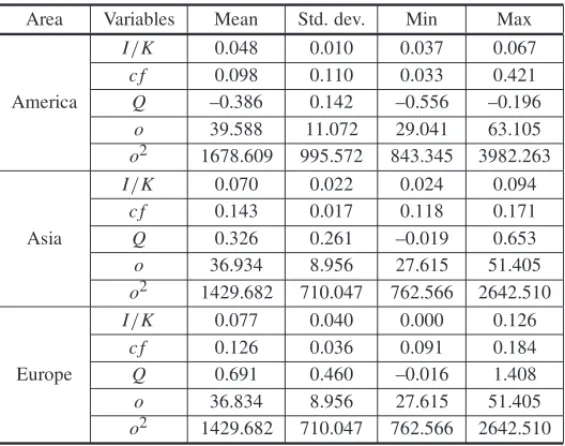
Descriptive statistics for the estimation sample is provided in Table 3.1. The mean averages of investment rate in North America, Asia and Europe are about 4, 7 and 8per cent respectively. Comparing with the investment rate in the 1990s in previous studies, which is around 18 per cent, the investment rates in all the three areas are relatively low.
Table 3.1– Descriptive Statistics of Estimation Sample.
Area Variables Mean Std. dev. Min Max
I/K 0.048 0.010 0.037 0.067
c f 0.098 0.110 0.033 0.421
America Q –0.386 0.142 –0.556 –0.196
o 39.588 11.072 29.041 63.105
o2 1678.609 995.572 843.345 3982.263
I/K 0.070 0.022 0.024 0.094
c f 0.143 0.017 0.118 0.171
Asia Q 0.326 0.261 –0.019 0.653
o 36.934 8.956 27.615 51.405
o2 1429.682 710.047 762.566 2642.510
I/K 0.077 0.040 0.000 0.126
c f 0.126 0.036 0.091 0.184
Europe Q 0.691 0.460 –0.016 1.408
o 36.834 8.956 27.615 51.405
o2 1429.682 710.047 762.566 2642.510
Table 3.2– Correlation Matrices of Variables.
Area I/K c f Q o
I/K 1
c f 0.166 1
America Q 0.030 0.287 1
o 0.467 –0.244 –0.133 1
o2 0.287 –0.239 –0.051 0.994 1
I/K 1
c f 0.605 1
Asia Q 0.630 0.814 1
o –0.217 –0.364 –0.374 1
o2 –0.179 –0.380 –0.364 0.997 1
I/K 1
c f 0.074 1
Europe Q –0.615 0.441 1
o 0.019 –0.480 –0.075 1
o2 0.051 –0.498 –0.115 0.997 1
4 EMPIRICAL RESULTS AND DISCUSSION
Table 4.1– OLS AR (1) Estimates for Model Variables.
Estimator I/K c f Q o o2
America –0.268 0.723 0.807** 0.103 0.121
(0.201) (0.586) (0.002) (0.762) (0.725)
Asia 0.771*** 0.722** 0.508 0.206 0.211
(0.000) (0.010) (0.130) (0.555) (0.545)
Europe 0.994*** 0.244 0.643** 0.206 0.211 (0.000) (0.465) (0.031) (0.555) (0.545)
OLS estimators obtained by EVIEWS 7.0; *Significant at 10, **5 and ***1
percent confidence level, respectively;p-values in brackets.
that significantly less than one into the simple autoregressive specifications. Therefore, a simple AR (1) specification is used to estimate the dynamic properties of the Q model. The AR (1) estimates for model variables with OLS estimators are presented in Table 4.1 below. The table reports the estimated coefficients on the lagged dependent variable from a simple AR (1) pro-cess: yt =r yt−1+µt. Some of the autoregressive parameters are significant below one, which
implies that the differenced variables contain information beyond that of a random walk. The autoregressive parameters significantly below one are Qin North America,I/K andC F/K in Asia, andI/KandQin Europe. The results not only show regional differences, but also provide information for modifications of Equation (5) in different regions. The modified equations and empirical results will be illustrated later in this chapter.
According to the AR (1) estimation, the explanatory variables should include all the explana-tory variables as well as the laggedQ. Hence, Equation (5) will transform into Equation (7), Equation (8), and Equation (9) to test Hypothesis One, Hypothesis Two, and Hypothesis Three, respectively:
I
K
t
=β0+β1Qt +β2Qt−1+β3c ft+β4ot+β5o2t +nt+γt (7)
I
K
t
=θ0+θ1
I
K
t−1
+θ2Qt+θ3c ft+θ4c ft−1+θ5ot+θ6o2t +nt+γt (8)
I
K
t =
ρ0+ρ1Qt+ρ2Qt−1+ρ3c ft +ρ4ot+ρ5o2t +nt+γt (9)
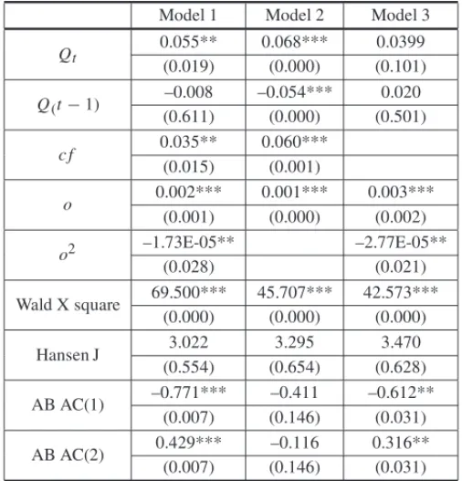
From the observation of Wald X, J-Statistic, and AB AC (n) (Arellano-Bond test), Model 2 performs the best among the first group of three models and achieves the results with the best significance level (the p-values of Qt, Qt−1andot are almost zero and that ofc ft is 0.001).
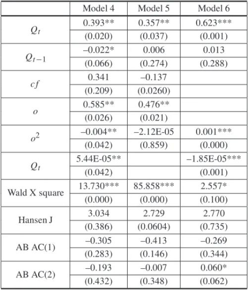
Model 4 presents the relationship the best among the second group of three models. The results of Model 4 suggest thatQt and lagged-term investment rate and cash flow rate are determinants
of the current year’s investment rate. In addition, the negative value ofot and positive value of
o2t construct aU shaped relationship between investment and oil price uncertainty in this area, which means that investment and oil price volatility are negatively correlated in the short term but are positively correlated in the long term. Model 8 performs the best in the third group. It indicates that different from the curve relationship results from the estimation of North America and Asia, the relationship between investment and oil price uncertainty in Europe shows a simple linear correlation. They are positively linked.
Table 4.2– America: Estimation Results, Dynamic Investment Models.
Model 1 Model 2 Model 3
Qt
0.055** 0.068*** 0.0399
(0.019) (0.000) (0.101)
Q(t−1)
–0.008 –0.054*** 0.020
(0.611) (0.000) (0.501)
c f 0.035** 0.060***
(0.015) (0.001)
o 0.002*** 0.001*** 0.003***
(0.001) (0.000) (0.002)
o2 –1.73E-05** –2.77E-05**
(0.028) (0.021)
Wald X square 69.500*** 45.707*** 42.573***
(0.000) (0.000) (0.000)
Hansen J 3.022 3.295 3.470
(0.554) (0.654) (0.628)
AB AC(1) –0.771*** –0.411 –0.612**
(0.007) (0.146) (0.031)
AB AC(2) 0.429*** –0.116 0.316**
(0.007) (0.146) (0.031)
The empirical results obtained by EVIEWS 7.0; *Significant at 10, **5 and ***1
percent confidence level, respectively;p-values in parentheses.
(1998), Sarkar (2000) and Folta & O’Brien (2004) in the estimation of strategic growth options and compound options. The results reveal a strategic investment rational of oil companies in this region that strategic growth options to invest overweights the compound options from other elements in facing the current high oil price volatility. They are eager to seize the opportunity to development during an oil price volatility-growing period; however, if the volatility keeps growing, they will consider reducing strategic investment.
Table 4.3– Asia: Estimation Results, Dynamic Investment Models.
Model 4 Model 5 Model 6
Qt
0.393** 0.357** 0.623***
(0.020) (0.037) (0.001)
Qt−1
–0.022* 0.006 0.013
(0.066) (0.274) (0.288)
c f 0.341 –0.137
(0.209) (0.0260)
o 0.585** 0.476**
(0.026) (0.021)
o2 –0.004** –2.12E-05 0.001***
(0.042) (0.859) (0.000)
Qt
5.44E-05** –1.85E-05***
(0.042) (0.001)
Wald X square 13.730*** 85.858*** 2.557*
(0.000) (0.000) (0.100)
Hansen J 3.034 2.729 2.770
(0.386) (0.0604) (0.735)
AB AC(1) –0.305 –0.413 –0.269
(0.283) (0.146) (0.344)
AB AC(2) –0.193 –0.007 0.060*
(0.432) (0.348) (0.062)
The empirical results obtained by EVIEWS 7.0; *Significant at 10, **5
and ***1 percent confidence level, respectively;p-values in parentheses.
price volatility. In addition, the different Value of Information and Value of Flexibility (Hayashi et al., 2007) could also contribute to the diverse curve of these two regions.
Table 4.4– Europe: Estimation Results, Dynamic Investment Models.
Model 7 Model 8 Model 9
Qt
0.396** 0.341*** 0.342*** (0.044) (0.004) (0.009)
Qt−1
0.009 0.0153 0.024*
(0.523) (0.195) (0.075)
c f –0.023 –0.026 –0.023
(0.230) (0.117) (0.211)
o 0.229 0.0120
(0.174) (0.129)
o2 0.0004 0.002*** 0.002**
(0.795) (0.001) (0.024)
Qt
1.80E-05 –4.22E-06
(0.431) (0.627)
Wald X square 3.059* 3.405* 0.301 (0.080) (0.065) (0.583)
Hansen J 3.156 3.308 3.258
(0.368) (0.508) (0.516)
AB AC(1) –0.527* –0.389 –0.302
(0.064) (0.172) (0.289)
AB AC(2) –0.119 –0.131 –0.297
(0.164) (0.348) (0.306)
The empirical results obtained by EVIEWS 7.0; *Significant at 10, **5
and ***1 percent confidence level, respectively;p-values in parentheses.
Therefore, Hypothesis Three fails to be rejected from the estimation of Europe as well. The results contrast to the findings of Glass & Cahn (1987) in the study of energy price movements and aggregate investment, and Mohn & Misund (2009) in the study of oil companies’ investment and market and oil price uncertainties from the firm’s level; but are in line with studies, such as Shaanan (2005) when detecting stock market uncertainty and investment of some groups of U.S. companies. It is shown that oil companies in Europe treated the growth of oil price volatility as a positive term.
From the analysis of the results drawn from the three regions, different relationships between oil price uncertainty and investment are found. In North America, this relationship shows a reverse
5 CONCLUSIONS
The purpose of this study is to estimate the impacts of oil price uncertainty on strategic invest-ments of oil exploration and production companies from a regional industrial level and to test whether the impacts vary in different regions. The finding of this study is that the regional va-riety does exist in the relationship between oil price uncertainty and strategic investment, as the empirical results of the three regions shows dramatic differences. The relationship between oil price uncertainty and strategic investment in North America shows a reversed U shaped curve; that in Asia shows aU shaped curve; that in Europe shows a positively correlated linear shape. The transaction cost economics – Tobin’sq theory is employed to form the original equation that assumes a positive relationship between strategic investment and Tobin’sQ. This positive relationship is proved by the results of North America, while a negative relationship is proved by the results of Asia and no meaningful empirical evidence is shown from the results of Europe. These findings are in line with some previous researches with the finding that a strong positive relationship between strategic investment and Tobin’sQis hard to achieve.
The agency theory is invited to justify the cash flow as a variable to adjust the original Tobin’s
qtheory. Therefore, in this study, the cash flow over capital stock ratio is invited as an optional variable utilized in model specifications. The results of three forms of model specifications can demonstrate the validity of cash flow variable in the equation. From the empirical results of each of the three regions, the cash flow variable plays an important role in the equation adjustment.
6 LIMITATIONS
The results of this study are limited by a relatively short period of data set. Availability of reli-able accessible data in Osiris and DataStream prohibited an extended review of the full sample. However, half of the crude oil exploration and production companies in Asia have only records from 2000. By removing all these companies, the sample would not be as representative as it currently is. Incorporating data from North American and European companies that extend from 90s would help rectify the imbalance sample.
REFERENCES
[1] ABELAB. 1983. Optimal investment under uncertainty.The American Economic Review,73: 228– 233.
[2] ALMEIDAATD & DUARTEM. 2011. A multi-criteria decision model for selecting project portfolio with consideration being given to a new concept for synergies.Pesquisa Operacional,31(2): 301– 318.
[3] ARELLANOM & BONDS. 1991. Some tests of specification for panel data: Monte Carlo evidence and an application to employment equations.Review of Economic Studies,58: 277–297.
[5] BERNANKEBS. 1983. Irreversibility, uncertainty and cyclical investment.Quarterly Journal of Eco-nomics,98: 85–106.
[6] BLOOMN. 2000. The real options effect of uncertainty on investment and labor demand. Working Study 00/15.Institute for Financial Studies, Nov. 2000.
[7] BLUNDELLRW & BONDSR. 1998. Initial conditions and moment restrictions in dynamic panel data models.Journal of Econometrics,87: 115–143.
[8] BRENNAN MJ & TRIGEORGISL. 2000. Real options: Development and new contributions. In: Project Flexibility, Agency, and Competition: New Developments in the Theory and Application of Real Options. Oxford University Press, USA, 1–9.
[9] BONDSR & CUMMINSJG. 2004. Uncertainty and company investment, an empirical model using data on analysts’ profits forecasts, Mimeo, Institute for Fiscal Studies.
[10] BONDS, KLEMM A, NEWTON-SMITHR, SYEDM & VLIEGHEG. 2004. The roles of expected profitability, Tobin’sQand cash flow in econometric models of company investment, Working study No. 222, Bank of England.
[11] BONDS & VANREENENJ. 2007. Micro econometric models of investment and employment. In: HECKMANJ & LEANERE (Eds.), Handbook of Econometrics, vol. 6A. Elsevier North Holland.
[12] BULANLT. 2005. Real options, irreversible investment and firm uncertainty, new evidence from U.S. firms.Review of Financial Economics,14: 255–279.
[13] CABALLERORJ. 1999. Aggregate investment. In: TAYLORJB & WOODFORDM (Eds.), Handbook of Macroeconomics, Vol. 1B. North-Holland, Amsterdam.
[14] CAMPAJ. 1993. Entry by foreign firms in the United States under exchange rate uncertainty.The Review of Economics and Statistics,75(4): 614–622.
[15] CARRUTHA, DICKERSONA & HENLEYA. 2000. What do we know about investment under un-certainty?Journal of Economic Surveys,14: 119–153.
[16] DALBEMMC, GOMESLL & BRANDAO˜ LET. 2014. Investors’asymmetric views and their decision to enter Brazil’s wind energy sector.Pesquisa Operacional,34(2): 319–345.
[17] DIASMAG. 2004. Valuation of exploration and production assets: an overview of real options mod-els.Journal of Petroleum Science and Engineering,44(1): 93–114.
[18] DIXITA & PINDYCKR. 1994. Investment under Uncertainty. Princeton University Press, Princeton.
[19] DRIVERC, YIPP & DAHKILN. 1996. Large company capital formation and effects of market share turbulence: micro-data evidence from the PIMS database.Applied Economics,28: 641–651.
[20] DRIESPRONGG, JACOBSENB & MAATB. 2008. Striking oil: Another puzzle?Journal of Financial Economics,89: 307–327.
[21] ELDERJ & SERLETISA. 2010a. Oil price uncertainty. Journal of Money,Credit and Banking,42: 1137–1159.
[22] ELDERJ & SERLETISA. 2010b. Oil price uncertainty in Canada.Energy Economics,31: 852–856.
[24] FAN Y & ZHUL. 2009. A real options based model and its application to China’s overseas oil. Energy Economics,32: 627–637.
[25] FAVERCA, PESARANMH & SHARMAS. 1992. Uncertainty and irreversible investment, an empir-ical analysis of development of oilfields on the UKCS. Working Study (EE17). Oxford Institute for Energy Studies.
[26] FLATHCM, BENOIT CR, ARNDH & LEOST. 2011. Strategic investment under uncertainty: A synthesis.European Journal of Operational Research,215: 639–650.
[27] FOLTATB & O’BRIENJP. 2004. Entry in the presence of dueling options.Strategic Management Journal,25: 121–138.
[28] GHOSALV & LOUGANIP. 1996. Product market competition and the impact of price uncertainty on investment: some evidence from US manufacturing industries.Journal of Industrial Economics,44: 217–228.
[29] GLASSV & CAHNES. 1987. Energy price uncertainty over the business cycle.Energy Economics, 9: 257–264.
[30] GOLDBERGL. 1993. Exchange rates and investment in United States industry.The Review of Eco-nomics and Statistics,75: 575–589.
[31] GOLFETORR, MORETTIAC & SALLESNETOLLD. 2009. A genetic symbiotic algorithm applied to the one-dimensional cutting stock problem.Pesquisa Operacional,29(2): 365–382.
[32] GRENADIERSR. 2002. Option exercise games: An application to the equilibrium investment strate-gies of firms.Review of Financial Studies,15(3): 691–721.
[33] GUISOL & PARIGIG. 1999. Investment and demand uncertainty.Quarterly Journal of Economics, 114: 185–227.
[34] HARTMANR. 1972. The effects of price and cost uncertainty on investment.Journal of Economic Theory,5: 258–266.
[35] HAYASHI SHD, LIGERO EL & SCHIOZERDJ. 2007. Decision-making process in development of offshore petroleum fields. In Latin American & Caribbean Petroleum Engineering Conference. Society of Petroleum Engineers.
[36] HENRIQUESI & SADORSKYP. 2011. The effect of oil price volatility on strategic investment.Energy Economics,33: 79–87.
[37] HUBBARDRG. 1998. Capital market imperfections and investment.Journal of Economic Literature, 36: 193–225.
[38] HURNAS & WRIGHTRE. 1993. Geology or economics? Testing models of irreversible investment using North Sea oil data.The Economic Journal,104(423): 363–371
[39] HUZINGAJ. 1993. Inflation uncertainty, relative price uncertainty, and investment in US manufactur-ing. Journal of Money,Credit and Banking,25: 521–557.
[40] JENSENMC & MECKLINGWH. 1976. Theory of the firm: managerial behavior, agency costs and ownership structure.Journal of Financial Economics,3: 305–360.
[42] LEAHYJV & WHITED TM. 1996. The effect of uncertainty on investment: some stylized facts. Journal of Money, Credit and Banking,28: 64–83.
[43] LEITELAM, TEIXEIRAJP & SAMANEZCP. 2012. Ex-ante economic assessment in incremental R&D projects: technical and development time uncertainties addressed by the real options theory. Pesquisa Operacional,32(3): 617–642.
[44] LOPESYG & ALMEIDA ATD. 2013. A multicriteria decision model for selecting a portfolio of oil and gas exploration projects.Pesquisa Operacional,33(3): 417–441.
[45] MAKADOKR. 2003. Doing the right thing and knowing the right thing to do: why the whole is greater than the sum of the parts.Strategic Management Journal,24: 1043–1055.
[46] MANKIWG. 2006. Macroeconomics, 6th ed. Worth Publishers.
[47] MCDONALDR & SIEGELD. 1986. The value of waiting to invest.The Quarterly Journal of Eco-nomics,101(4): 707–728.
[48] MOHNK & MISUNDB. 2009. Investment and uncertainty in the international oil and gas industry. Energy Economics,31(2): 240–248.
[49] MOHNK & OSMUNDSENP. 2006. Uncertainty, asymmetry and investment, an application to oil and gas exploration. Working Study, University of Stavanger.
[50] MUNJ. 2006. Real Option Analysis: Tools and Techniques for Valuing Strategic Investments and Decisions. 2nd ed.New Jersey: John Wiley & Son.19–50.
[51] MIEGHEMJA. 2003. Commissioned study: Capacity management, investment, and hedging: Review and recent developments.Manufacturing & Service Operations Management,5(4): 269–302.
[52] MYERSSC & TURNBULLSM. 1977. Capital budgeting and the capital asset pricing model: good news and bad news.The Journal of Finance,32(2): 321–333.
[53] NARAYANPK & SHARMASS. 2011. New evidence on oil price and firm returns.Journal of Banking & Finance,35(12): 3253–3262.
[54] NOVAESAG & SOUZAJC. 2005. A real options approach to a classical capacity expansion problem. Pesquisa Operacional,25(2): 159–181.
[55] OGAWAK & SUZUKIK. 2000. Uncertainty and investment: some evidence from the panel data of Japanese manufacturing firms.Japanese Economic Review,51: 170–192.
[56] PADDOCKJL, SIEGELDR & SMITHJL. 1988. Option valuation of claims on real assets: the case of offshore petroleum leases.Quarterly Journal of Economics,103: 479–508.
[57] PINDYCKR. 1991. Irreversibility, uncertainty and investment.Journal of Economic Literature,29: 1110–1148.
[58] POMPERMAYERFM, FLORIAN M, LEAL JE & SOARESAC. 2007. A spatial price equilibrium model in the oligopolistic market for oil derivatives: an application to the Brazilian scenario.Pesquisa Operacional,27(3): 517–534.
[59] PORTERME. 1980. Competitive Strategy. Free Press, New York.
[60] REGNIERE. 2006. Oil and energy price volatility.Energy Economics,29(1): 405–427.
[62] ROSSS. 1978. A simple approach to the valuation of risky streams.Journal of Business,51(3): 453– 475.
[63] SADORSKYP. 2004. Stock markets and energy prices.Encyclopedia of Energy, vol. 5. Elsevier, New York, 707–717.
[64] SADORSKYP. 2008. Assessing the impact of oil prices on firms of different sizes: its tough being in the middle.Energy Policy,36: 3854–3861.
[65] SANT’ANNAAP. 2002. Data envelopment analysis of randomized ranks.Pesquisa Operacional, 22(2): 203-215.
[66] SARKARS. 2000. On the investment–uncertainty relationship in a real options model.Journal of Economic Dynamics and Control,24: 219–225.
[67] SHAANANJ. 2005. Investment, irreversibility, and options: an empirical framework.Review of Fi-nancial Economics,14: 241–254.
[68] SILVATADO & SANTIAGOLP. (2009). New product development projects evaluation under time uncertainty.Pesquisa Operacional,29(3): 517–532.
[69] SMITHJE & MCCARDLEKF. 1999. Options in the real world: lessons learned in evaluating oil and gas investments.Operations Research,47: 1–15.
[70] SMITTJ & TRIGEORGISL. 2004. Strategic Investment, Real Options and Games. Princeton Univer-sity Press, New Jersey.
[71] SOLPD & GHEMAWATP. 1999. Strategic valuation of investment under competition.Interfaces, 29(6): 42–56.
[72] SUSLICKSB, SCHIOZERD & RODRIGUEZMR. 2009. Uncertainty and risk analysis in petroleum exploration and production.Terræ,6(1): 30–41.
[73] TOBINJ. 1969. A general equilibrium approach to monetary theory.Journal of Money, Credit, and Banking,1: 15–29.