Página | 172
https://periodicos.utfpr.edu.br/rbgeo
Chebyshev norm adjustment: what to
expect? Case study in a leveling network
ABSTRACT
Stefano Sampaio Suraci
orcid.org/0000-0002-4453-9273
Instituto Militar de Engenharia (IME), Rio de Janeiro, Rio de Janeiro, Brasil.
Leonardo Castro de Oliveira
[email protected] orcid.org/0000-0001-5290-5029
Instituto Militar de Engenharia (IME), Rio de Janeiro, Rio de Janeiro, Brasil.
This work drew attention to the Chebyshev norm minimization, a method of adjustment of observations still little explored in the geodetic literature. Chebyshev norm minimization refers to the minimization of the maximum weighted absolute residual of adjusted observations. In addition to contributions to the formulation of Chebyshev norm adjustment by linear programming, numerical examples of its application in a leveling network were presented and compared with the respective Least Squares adjustments in this work. We verified that residuals analysis of Chebyshev norm adjustment is even less effective than of Least Squares for outlier identification. We also highlighted other characteristics of the method that had never been explored in geodetic literature before. In special, Chebyshev norm adjustment presented lower maximum absolute residual, and more homogeneous absolute residuals than LS when applied with the usual distance-dependent stochastic model. More experiments should be conducted in future work to confirm these tendencies. We also analyzed the adjustment by Chebyshev norm minimization with unit weights, which generates the minimum maximum absolute residual for a network. As some characteristics of Chebyshev norm adjustment seen promising, other suggestions for future work were also made.
Página | 173
INTRODUCTION
In the estimation of geodetic networks, the number of observations is higher than that of unknowns. This is the basis for assessing the precision and reliability of geodetic networks through redundancy. The inevitable measurement errors make the system inconsistent (GEMAEL et al., 2015). Network adjustment is usually performed by the Least Squares (LS) method, which minimizes the sum of the squared elements of the residual vector v, weighted by weight matrix of observations P (Equation 1). Its results have the minimum variance for the estimated parameters, and maximum likelihood, considering the occurrence of only random errors normally distributed in the observations (GHILANI, 2010).
LS: min ሺvTPvሻ (1)
Another possible minimization of vector norm, less established in the geodetic literature, involves the adjustment by Chebyshev Norm Minimization (CNM). CNM adjustment refers to the minimization of the maximum weighted absolute residual (MWAR) of observations. For uncorrelated (independent) observations, being m the number of observations, and p the weight vector composed of the elements of the main diagonal of P, MWAR and the CNM adjustment are expressed by Equations 2 and 3, respectively. In leveling networks observations are usually independent, and their weights pi are commonly given
by the inverse of the length of the respective leveling line (GHILANI, 2010).
MWAR=max(pi*|vi|), 1≤i≤m (2)
CNM: minሺMWARሻ=min(max (pi*|vi|) ), 1≤i≤m (3)
In the context of leveling networks, Ebong (1986) was the only work on CNM that has been found. In that paper the author has suggested that the method can provide an adjustment with no significant bias, and information about errors in
observations with quality equivalent to LS. However, LS does have other
advantages previously mentioned, such as minimum variance and maximum likelihood. Hence, probably that is the reason why there has been no other paper on CNM in geodetic networks since 1986, year of publication of that one. Besides, later, in the context of polynomial approximation, Abdelmalek and Malek (2008) showed that the adjustment by CNM tends to distribute errors of outliers among other observations even more than LS. Therefore, it is even less effective than LS for outlier identification. This was confirmed in a leveling network in our experiments.
Then we investigated the application for CNM in networks with no outliers. Since CNM tends to distribute errors even more than LS, it may be subject of investigation if this provides more homogeneous results for the adjustments,
Página | 174
something that may be useful under the premise of non-existence of outliers. This point, not previously addressed in the literature, was also tested in the experiments.
However, there is also a specific CNM adjustment, not explored yet in the geodetic literature, which provides other interesting outcome: the minimization of the maximum absolute residual (MAR). This can be achieved in the adjustment by CNM with unit weights for all observations. Thus, minimization occurs in the absolute residual vector |v|, i.e., the MAR (Equation 4) of the network is minimized. This means an adjustment with minimum maximum distortion of observed values. Consequences of this property for the adjustment were analyzed in the experiments as well.
MAR=max|vi|, 1≤i≤m (4)
For independent observations (general case of leveling networks), weights of observations are relative, so that multiplying them all by the same scale factor does not change the estimated parameters and residuals of the adjustment. Hence, MAR minimization is obtained for any stochastic model with equal weights, not necessarily the unit ones.
Finally, the suggestion that a network is "free of outliers" is ambiguous. In this research we considered a network to be free of outliers if none was identified by data snooping iterative procedure (Teunissen, 2006) with significance level of 0.001. For a review on data snooping procedure we recommend (Rofatto et al., 2018). However, it depends on the perspective defended by the geodesist on the issue.
MODEL DESCRIPTION
In this section, we presented the formulation of the adjustment of observations by CNM for implementation by the SIMPLEx linear programming method. We considered that the system of equations is linear and that the observations to be adjusted are independent (the matrix of weights P is diagonal). The occurrence of such premises is common in leveling networks and was the case in the experiments of this research. Further details on linear programming and SIMPLEx can be found in Dantzig (1963) and Amiri-Simkooei (2003).
The content of this section was based on the L1 norm minimization formulation by Amiri-Simkooei (2003). The necessary adaptations for CNM were inspired by Ebong (1986) and Abdelmalek and Malek (2008). In addition to greater detailing specifically for the case of geodetic networks, the main contribution presented here is the inclusion of weights of observations in the formulation.
The functional model of Gauss-Markov Model is defined by Equation 5, where Amxn is the coefficients matrix of the network parameters (unknowns) vector xnx1, Lmx1 is the vector of observed values, and vmx1 is the vector of
Página | 175
residuals, being m the number of observations, and n the number of unknowns. Datum constraints and not fixed control station heights may be added to the model by different approaches as presented in Ghilani (2010).
Ax=L+v (5)
As we could see in Equation 3, for the adjustment by CNM the maximum value among the weighted (by means of the weights vector pmx1, composed of the elements of the main diagonal of P) absolute residuals must be minimized. In order to solve this linear programming minimization problem using the SIMPLEx method, all variables xi and vi (components of vectors x and v, respectively) need
to be non-negative. Since residuals and network parameters in practice do not have signal constraint, artificial variables must be inserted for x and v (Equation 6) to address such limitation. As a consequence, the elements pi*|vi| of Equation 3 are given by Equation 7. Therefore, after solving the problem for the non-negative variables αi, βi, ui, and wi, and returning to the originals xi and vi, the latter can assume negative values. Vectors α and β have same dimensions of x, and u and w as of v.
x=α-β;v=u-w (6)
pi*|vi|=(pi*ȁui-wiȁ), 1≤i≤m (7)
Then, a one-dimensional variable s is created, which must be minimized and characterize the objective function (Equation 8), being 02(n+m)x1 a vector of zeros, and [1]1x1 a matrix whose unique element is "1". The strategy is to impose that each element pi*|vi| is less than or equal to s, by means of constraints of the problem of linear programming (Equation 9). In the latter, 0mxn (left side of the inequality) are matrices of zeros, 02mx1 (right side of the inequality) is a vector of zeros, Pmxm is the weight matrix of observations, and [-1]mx1 is a vector whose elements are all equal to " -1".
f=ሾ0T ሾ1ሿሿ ۏ ێ ێ ۍαβ u w s ے ۑ ۑ ې →min (8) 0 0 -P P ሾ-1ሿ 0 0 P -P ሾ-1ሿ൨ ۏ ێ ێ ۍαβ u w s ے ۑ ۑ ې ≤0 (9)
Página | 176
The other constraints of the problem are presented in Equation 10, where
Imxm is an identity matrix, and 0smx1 is a matrix of zeros. They are equivalent to the functional model of Equation 5 but with adaptations to the standard linear programming format. In order to be consistent with the constraints of Equation 9 and with the objective function (Equation 8), variable s needed to be included in Equation 10 as well. Since s does not participate in the functional model, its respective column 0S has all elements equal to zero.
ሾA -A -I I 0Sሿ ۏ ێ ێ ۍαβ u w s ے ۑ ۑ ې =ሾLሿ (10) METHODOLOGY
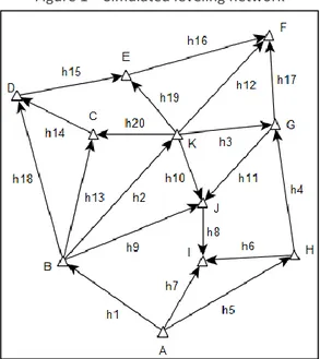
In the experiments a leveling network initially with no outliers was simulated. The simulated network is shown in Figure 1 and Table 1. The height of A was considered fixed and with value hA=0. Thus, it is a network with 20 observations and 10 heights to be determined (unknowns), that is, the number of degrees of freedom is 10. Observations were simulated with only random errors (normal distribution). The standard deviation σi of the observations adopted in
the simulations is given by Equation 11, where K (in km) is the length of the respective leveling line.
σi=1.0(mm)*ඥKi (11)
Figure 1 – Simulated leveling network
Página | 177
In the first experiment, an outlier was purposely inserted in the sample of observations of the simulated network, in order to confirm that residuals analysis of CNM is even less effective than of LS for outlier identification. This was verified by comparing the residual of the outlier with residuals of the other observations of the network in CNM, and with its residual in the LS adjustment. The usual 3σ-rule for outlier identification was applied. Both adjustments considered the usual distance-dependent approach for the weights of observations.
Table 1 – Observations of the simulated network hi Distance (km) Value (mm) σi (mm) hi Distance (km) Value (mm) σi (mm) h1 49 163842.9 7.00 h11 62 110222.7 7.87 h2 41 6454.3 6.40 h12 50 155935.7 7.07 h3 38 57028.5 6.16 h13 35 52872.4 5.92 h4 34 126217.1 5.83 h14 43 62894.6 6.56 h5 22 101138.5 4.69 h15 20 3887.6 4.47 h6 13 296883.4 3.61 h16 28 42706.4 5.29 h7 23 398019.8 4.80 h17 19 98890.6 4.36 h8 48 60443.6 6.93 h18 39 115772.5 6.24 h9 15 173717.6 3.87 h19 27 113219.9 5.20 h10 24 167271.4 4.90 h20 21 46430.1 4.58
Source: Own authorship (2019).
The second experiment was conducted in the initial simulated network with no outliers. We performed four different adjustments, two by CNM (Adj 1 and 2), and two by LS (Adj 3 and 4) for comparison:
a) CNM with stochastic modeling in the distance-dependent approach,
which establishes the weights of observations as inversely proportional to the length of the respective leveling lines (Adj 1);
b) CNM with unit (equal) weights for network observations (Adj 2);
c) LS with stochastic modeling in the distance-dependent approach (Adj 3);
d) LS with unit (equal) weights for network observations (Adj 4).
We separately compared the MWAR of Adj 1 and 3, and Adj 2 and 4, to demonstrate the MWAR minimization characteristic of the adjustments by CNM over the results by LS. We also compared the MAR of these four adjustments, in order to illustrate that Adj 2 provides the minimum MAR for the network.
Based on the numerical results, we highlighted a property of the CNM that results in the repetition of weighted residuals equal to MWAR. We also validated the point that any adjustment by the CNM with equal weights leads to the minimization of the MAR. Finally, we compared the mean and the standard deviation of absolute residuals, and the discrepancy between the largest and the smallest absolute residual of the four adjustments, for further analysis.
The experiments were performed using the software Octave (version 4.2.1) in an Intel(R) Core(TM) i3 CPU. Linear programming problems were solved by the
SIMPLEx method, using the glpk routine. For the simulation of random numbers
(with normal distribution) we used the randn routine, which applies the Ziggurat technique (MARSAGLIA; TSANG, 2000). The reader can contact the authors to obtain the Octave codes of the experiments.
Página | 178
NUMERICAL RESULTS
EXPERIMENT 1 – LEVELING NETWORK WITH ONE OUTLIER
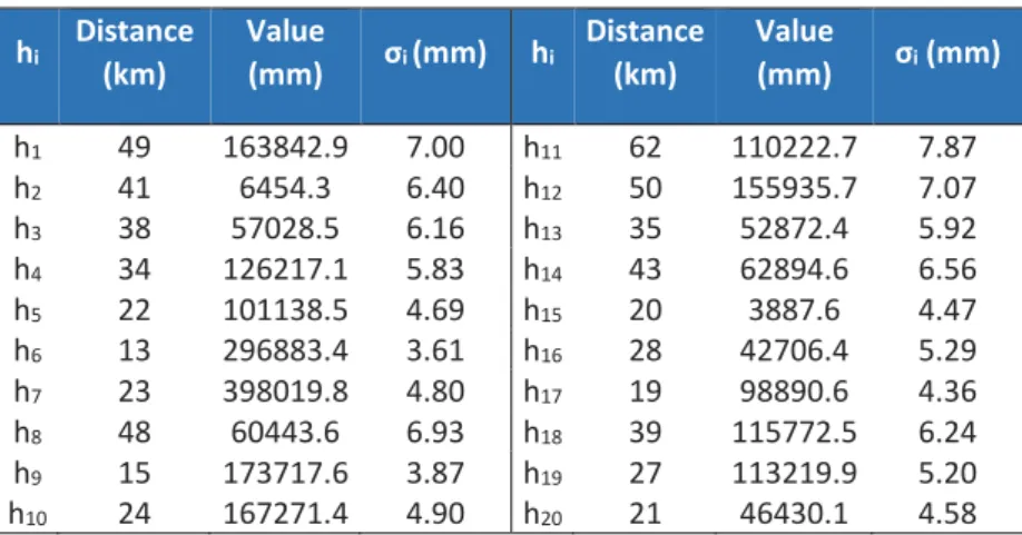
In order to perform this experiment, a gross error of 50 mm was purposely added to h5, generating a simulated outlier in the data. Table 2 shows the residual vector v of CNM and LS adjustments. Absolute residuals higher than 3σi were marked with an asterisk.
Table 2 – Residuals (mm) – Experiment 1
vi CNM LS vi CNM LS v1 -20.23 25.49* v11 -24.25* 2.35 v2 15.69 -1.69 v12 0.47 -4.65 v3 34.13* 14.18 v13 8.83 7.68 v4 -30.54* -15.39 v14 -6.79 4.03 v5 -19.76* -26.53* v15 17.97* 5.06 v6 -11.68* -9.79 v16 25.15* 5.89 v7 20.66* 15.77* v17 -17.07* -2.23 v8 43.12* 3.24 v18 -3.46 6.21 v9 13.47* 2.74 v19 -15.28 -1.15 v10 -10.32 -3.67 v20 -18.86* -2.64
Source: Own authorship (2019).
We can verify that both CNM and LS adjustments distributed residuals of the outlier among other “good” observations. However, the outlier absolute residual was higher in LS than in CNM. In addition, the outlier absolute residual was the highest in LS adjustment, while it was only the eighth highest in CNM. Hence, based on residuals analysis, LS adjustment presented better conditions for the outlier identification to be viable.
Besides, considering the 3σ-rule, LS identified three outliers, and CNM identified twelve, while there was only one in the data. Hence, even though both CNM and LS identified correctly the outlier, CNM had a higher number of false positives. Therefore, residuals analysis of CNM proved to be even less effective than of LS for outlier identification.
EXPERIMENT 2 – LEVELING NETWORK WITHOUT OUTLIERS
Experiment 2 was performed in the initial simulated network of Figure 1 and Table 1. No outliers were identified in the network, considering the data
snooping iterative procedure with significance level of 0.001. Table 3 presents the
MWAR comparison of the adjustments with weights of the observations in the distance-dependent approach (Adj 1 and 3), and the same is done in Table 4 for unit weights (Adj 2 and 4). In both cases, the adjustment by CNM presented lower MWAR than by LS, as expected, which confirms its main characteristic. About units of measurement, since we dealt with residuals vi in mm, and weights
of observations pi in 1/mm2 (mm-2), the unit of MWAR (Equation 2) was 1/mm
Página | 179
Table 3 – MWAR – Experiment 2 – distance-dependent weights Adj 1 Adj 3
MWAR (mm-1) 0.21 0.29
Source: Own authorship (2019). Table 4 – MWAR – Experiment 2 – unit weights
Adj 2 Adj 4
MWAR (mm-1) 6.98 11.32
Source: Own authorship (2019).
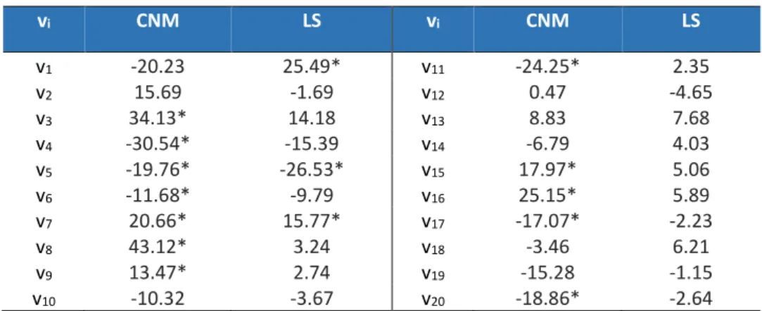
Several weighted absolute residuals in Adj 1 and 2 were equal to the MWAR of the respective adjustment, which is a property of the adjustments by CNM. For this experiment 2, the repetition of MWAR in each adjustment by CNM occurred 11 times, that is, 11 observations had absolute weighted residual equal to the MWAR. Further details on such property of the adjustment by CNM can be found in Abdelmalek and Malek (2008). This property was seen in all CNM adjustments of our paper.
Table 5 shows the residual vector v of the four adjustments. We can verify said repetition of the MWAR in Adj 2, because in this case (unit weights) the MWAR numerically coincides with the MAR (disregarding units of measurements). We also performed other adjustments by CNM with equal but not unit weights. Results for the residuals were identical to those of Adj 2, which confirms that the minimization of the MAR by CNM is obtained with any stochastic model that consider the weights of observations to be equal, even if not unit weights.
Table 5 – Residuals (mm) – Experiment 2
vi Adj 1 Adj 2 Adj 3 Adj 4
v1 10.32 6.98 11.96 8.83 v2 -0.21 1.97 -4.18 -2.55 v3 8.00 6.98 10.86 11.32 v4 -7.16 -6.98 -7.28 -6.50 v5 -4.63 -6.98 -3.98 -5.81 v6 -2.31 -2.10 0.43 0.69 v7 -4.84 -6.98 -1.45 -3.02 v8 -2.30 -1.35 1.44 2.33 v9 2.84 3.08 0.85 1.52 v10 -5.05 -6.98 -3.07 -4.03 v11 7.15 6.23 6.27 4.85 v12 -10.32 -6.98 -6.29 -5.32 v13 7.37 6.98 6.08 6.20 v14 2.13 3.03 3.91 2.96 v15 4.21 6.98 4.12 6.62 v16 4.77 6.98 4.41 5.35 v17 -1.72 2.63 -0.56 -0.03 v18 3.99 4.52 4.49 3.66 v19 -5.68 -4.57 -1.31 -1.27 v20 -4.42 -6.98 -1.74 -3.25
Página | 180
Table 6 compares the MAR of the four adjustments. Adj 2, also as expected, presented the lowest MAR among them. It is worth mentioning that Adj 1 obtained lower MAR than the equivalent via LS (Adj 3). This result suggests that CNM tends to generate a lower MAR in general, even when equal weights are not adopted.
Table 6 – MAR – Experiment 2
Adj 1 Adj 2 Adj 3 Adj 4
MAR (mm) 10.32 6.98 11.96 11.32
Source: Own authorship (2019).
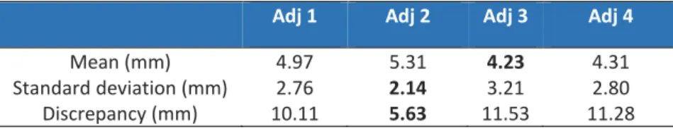
Table 7 presents some statistics of the absolute residuals of the four adjustments. Besides lower MAR, Adj 2 also implied a minimization of the standard deviation of absolute residuals, and minimization of the discrepancy between the largest and the smallest absolute residual of the adjustment. On the other hand, the mean of absolute residuals of Adj 2 was the highest among the four adjustments. Adj 1 had these same results, if compared only to its equivalent via LS (Adj 3). Hence, we can see that CNM tended to generate more homogeneous absolute residuals, but with a higher average value in general.
Table 7 – Statistics of absolute residuals – Experiment 2 Adj 1 Adj 2 Adj 3 Adj 4
Mean (mm) 4.97 5.31 4.23 4.31
Standard deviation (mm) 2.76 2.14 3.21 2.80
Discrepancy (mm) 10.11 5.63 11.53 11.28
Source: Own authorship (2019).
DISCUSSION
In Experiment 1, we confirmed that CNM is even less effective than LS for outlier identification. About Experiment 2, in agreement with its main characteristic of MWAR minimization, the adjustment by CNM presented lower MWAR than that by LS for the analyzed network, both with distance-dependent stochastic modeling, and adopting unit weights for observations. The MWAR repeating property for some of the weighted residuals was verified in the adjustments by CNM.
These properties had not been explicitly demonstrated previously in the geodetic literature, not even by Ebong (1986), but they seen not to have any practical advantage over LS. However, some results of the experiments showed that CNM adjustment does have some advantages.
With the usual distance-dependent weights, CNM presented lower MAR, and absolute residuals more homogeneous than LS. However, the average absolute residual was higher than in LS. It suggests that CNM increases the homogeneity of the network, at the expense of an increase in the average absolute residual.
A lower MAR can be considered an advantage, as it means a lower maximum distortion of observed values. A better homogeneity is especially relevant in the case of leveling networks, since their amount of constraints is usually relatively low. In the case of the High Precision Altimeter Network of the Brazilian Geodetic
Página | 181
System, for example, there is only one constraint for the stretch that covers most of the Brazilian territory. As the distance from the constraint increases, this tends to generate benchmarks with worse precisions than others, as seen in IBGE (2018). Hence, CNM homogeneity of results may be useful to minimize this effect.
In the adjustment by CNM with unit weights (Adj 2), the MAR numerically coincides with the MWAR (disregarding units of measurements). Thus, the MAR is also minimized in such adjustment. Adj 2 results were also the most homogeneous, but had the highest average absolute residual among the four adjustments analyzed. We also have shown that the minimization of the MAR is obtained with any stochastic model of equal weights for observations, not necessarily unit ones.
CONCLUSION
This work drew attention to the Chebyshev norm minimization, a method of adjustment of observations still little explored in the geodetic literature. Among others, we presented with numerical examples its main characteristic, which is the minimization of the MWAR of observations. We also approached the formulation of CNM for linear programming implementation via SIMPLEx method, with contributions and greater detail in relation to previous works. Based on the results of Experiment 1, we suggest that CNM adjustment is appropriate for networks in which possible outliers have been previously treated, because CNM proved to be even less effective than LS for outlier identification. All experiments were conducted in leveling networks.
In Experiment 2, we could see that the adjustment by CNM tended to lower the MAR of the observations, an advantage over LS. It also implied a smaller discrepancy between the maximum and minimum values of absolute residuals, and lower standard deviation of absolute residuals. This increase in the network homogeneity may be especially relevant for leveling networks. These effects were even more expressive when equal weights were adopted for all observations. Actually, CNM with equal weights generates the minimum MAR of a network, which can be evaluated as a possible metric of the quality of the adjustment in future work. Besides, the tendency of decreasing the MAR, and improving the homogeneity in CNM even with not equal weights suggested in this work should be verified with more experiments using Monte Carlo Simulation in future work.
However, differently from LS, the adjustment by CNM does not yet have a consolidated error propagation theory. Therefore, future work should be developed in order to allow the estimation of the precision of residuals and parameters estimated in the adjustment by CNM. The minimization of MAR and of standard deviation of absolute residuals in the adjustment may generate a better homogeneity between the standard deviation of leveling network estimated parameters, for example. Other practical advantages may be revealed as well.
It is also subject to investigation the application of results of a "pre-adjustment" of the network by CNM in the construction of the stochastic model for the adjustment itself by LS. It may contribute to the reduction of the MAR of
Página | 182
the adjustment, without giving up the advantages of the LS. Finally, the formulation and the experiments carried out in this research can be continued, with their extension to other types of geodetic networks.
Página | 183
Ajustamento pela norma de Chebyshev: o
que esperar? Estudo de caso em uma rede
de nivelamento
RESUMO
Este trabalho tratou da minimização da norma de Chebyshev, um método de ajustamento ainda pouco explorado na literatura geodésica. A minimização da norma de Chebyshev corresponde à minimização do máximo resíduo absoluto ponderado das observações ajustadas. Além de contribuições para a formulação do ajustamento pela norma de Chebyshev por programação linear, exemplos numéricos de sua aplicação em uma rede de nivelamento foram apresentados e comparados com os respectivos ajustamentos pelo Método dos Mínimos Quadrados. Foi verificado que a análise de resíduos do ajustamento pela norma de Chebyshev é ainda menos apropriada para a identificação de outliers que aquela por Mínimos Quadrados. Outras características ainda não exploradas na literatura geodésica do método também foram apresentadas. Em especial, o ajustamento pela norma de Chebyshev apresentou menor resíduo máximo absoluto e maior homogeneidade entre os resíduos absolutos, quando aplicado com o usual modelo estocástico com pesos pelo inverso da distância das linhas de nivelamento. Mais experimentos devem ser conduzidos em trabalhos futuros para confirmar essas tendências. O ajustamento pela norma de Chebyshev com pesos iguais, que gera o mínimo máximo resíduo absoluto para a rede, também foi analisado. Dado que algumas características do ajustamento pela norma de Chebyshev parecem promissoras, outras sugestões para trabalhos futuros foram apresentadas.
PALAVRAS CHAVE: Norma de Chebyshev. Ajustamento das observações. Rede de nivelamento.
Página | 184
REFERÊNCIAS
ABDELMALEK, N.; MALEK, W.. Numerical linear approximation in C. London: CRC Press, 2008, 928p.
AMIRI-SIMKOOEI, A.. Formulation of L1 Norm Minimization in Gauss-Markov
Models. Journal of Surveying Engineering, p.37-43, fev. 2003.
https://doi.org/10.1061/(ASCE)0733-9453(2003)129:1(37).
DANTZIG, G.. Linear Programming and Extensions. Princeton: Princeton University Press, 1963. 656p.
EBONG, M. B.. The Chebyshev adjustment of a geodetic levelling network. Survey
Review, v. 28, n. 220, p.315-321, 1986.
https://doi.org/10.1179/sre.1986.28.220.315.
GEMAEL, C.; MACHADO, A. M. L.; WANDRESEN, R.. Introdução ao ajustamento
de observações: aplicações geodésicas. 2. ed. Curitiba: Ed. UFPR, 2015. 428p.
GHILANI, C.. Adjustment Computations: Spatial Data Analysis. 5. ed. Hoboken: John Wiley & Sons, 2010. 647p.
IBGE. Reajustamento da Rede Altimétrica com Números Geopotenciais 2018. Instituto Brasileiro de Geografia e Estatística, 2018. 47p.
MARSAGLIA, G.; TSANG, W. W.. The Ziggurat Method for Generating Random
Variables, Journal of Statistical Software, v. 5, n. 8, 2000.
https://doi.org/10.18637/jss.v005.i08.
ROFATTO, V. F. et al.. A half-century of Baarda’s concept of reliability: a review,
new perspectives, and applications, Survey Review, 2018.
https://doi.org/10.1080/00396265.2018.1548118.
TEUNISSEN, P.. Testing theory: an introduction. 2. ed. Series on Mathematical Geodesy and Positioning, Delft: Delft Univ. of Technology, 2006. 147p.
Página | 185
Recebido: 20 fev. 2019
Aprovado: 01 out. 2019
DOI: 10.3895/rbgeo.v7n4.9627
Como citar: SURACI, S. S.; OLIVEIRA, L. C. Chebyshev norm adjustment: what to expect? Case study in a
leveling network. R. bras. Geom., Curitiba, v. 7, n. 4, p. 172-185, out/dez. 2019. Disponível em: <https://periodicos.utfpr.edu.br/rbgeo>. Acesso em: XXX.
Correspondência: Stefano Sampaio Suraci
Praça General Tiburcio, 80, Urca, CEP 22290-270, Rio de Janeiro, Rio de Janeiro, Brasi.
Direito autoral: Este artigo está licenciado sob os termos da Licença Creative Commons-Atribuição 4.0