MINIMIZATION OF ℓ₂-NORM OF THE KSOR OPERATOR

© 2012 Science Publications

doi:10.3844/jmssp.2012.461.470 Published Online 8 (4) 2012 (http://www.thescipub.com/jmss.toc)

Corresponding Author: Youssef, I.K.,Department of Mathematics, Faculty of Science, Ain Shams University, Cairo, 11566, Egypt

MINIMIZATION OF

ℓ

₂

_{-NORM OF THE KSOR OPERATOR}

Youssef, I.K. and A.I. Alzaki

Department of Mathematics, Faculty of Science, Ain Shams University, Cairo, 11566, Egypt Received 2012-08-17, Revised 2012-11-19; Accepted 2012-11-19

ABSTRAC

We consider the problem of minimizing the ℓ_{2-norm of the KSOR operator when solving a linear systems of}

the form AX = b where, A = I +B (TJ = -B, is the Jacobi iteration matrix), B is skew symmetric matrix. Based on the eigenvalue functional relations given for the KSOR method, we find optimal values of the relaxation parameter which minimize the ℓ_{2-norm of the KSOR operators. Use the Singular Value}

Decomposition (SVD) techniques to find an easy computable matrix unitary equivalent to the iteration matrix TKSOR. The optimum value of the relaxation parameter in the KSOR method is accurately approximated through the minimization of the ℓ_{2-norm of an associated matrix} ∆₍ω*_{) which has the same}

spectrum as the iteration matrix. Numerical example illustrating and confirming the theoretical relations are considered. Using SVD is an easy and effective approach in proving the eigenvalue functional relations and in determining the appropriate value of the relaxation parameter. All calculations are performed with the help of the computer algebra system “Mathematica 8.0”.

Keywords:KSOR Iterative Method, ℓ_{2-Norm, Singular Value Decomposition (SVD)}

1. INTRODUCTION

We consider linear systems of the form Equation 1: m

ij j

j j i 1

i

a x b , a 0,i 1, 2, , m =

= ≠ =

∑

⋯ (1)

With aij = - aji for i ≠ j and the system admits a unique solution. This system of equations can be written as Equation 2:

m m m

A X=b, AX, b∈R , A∈R × (2) Such linear systems arise in many different applications for example in the finite difference treatment of the Korteweg de Vries equation, Buckley (1977). Also, simi-lar linear systems appears in the treatment of coupled harmonic equations, Ehrlich (1972). In the iterative treatment of linear systems, we use the splitting, A = D-L-U, where D = d×Im is the diag-onal part of A, for some non-zero constant d, -L is the strictly lower-triangular part of A and -U is the strictly upper-triangular part of A, Woznicki (2001).

1.1.

Jacobi Method

Equation 3:

[ ] i 1 [ ] m [ ]

n 1 n n

i i ij j ij j

j 1 j i 1 ii

1

x b a x – a x

a − +

= + =

 

= _ − _



∑

∑

 (3)

The Jacobi Method in matrix form is Equation 4:

[ n 1] [n ] 1 1

J j

X + =T X +D b T− =D (L− +U) (4)

TJ is the Jacobi iteration matrix, it is clear that TJ in this case is a skew symmetric matrix.

1.2. The SOR Method is

Equation 5:

[ ] [ ] i 1 m

n 1 n [ n 1] [n ] [ n ]

i i i ij j ij j ii i

j 1 j i 1 ii

updated components old components

x x b a x a x a x

a

i 1, 2, , m; n 0, 1, −

+ +

= = +

 

 

ω_{ }

= + − − −

 

 

 

= =

∑

∑

⋯ ⋯

where, ω∈ (0,2) is a relaxation parameter, ω = 1 gives the well-known Gauss-Seidel method.

The SOR Method in matrix form is Equation 6:

(

)

(

[ n 1] [n ] 1 SOR

1 SOR

X T X (D L) b

T (D L) 1 D U)

+ −

−

= + − ω ω

= − ω − ω + ω (6)

where, TSOR is the SOR iteration matrix.

The choice of the relaxation parameter ω is very important for the convergence rate of the SOR method. For certain classes of matrices (2-cyclic consistently ordered) with property A, in the sense of Young (2003), for such systems there is a functional eigenvalue relation of the form Equation 7:

(

)

1/ 2

1

λ + ω − = ωµλ (7)

where, λ is an eigenvalue of the TSOR and µ is a corresponding eigenvalue of the TJ. Most work on the choice of ω is to minimize ρ(TSOR) which is only an asymptotic criteria of the convergence rate of linear stationary iterative method, Hadjidimos and Neumann (1998). In real computations, we have to consider average convergence rate Milleo et al. (2006). The determination of the optimal value of the relaxation parameter ωopt can be obtained with the help of the eigenvalue functional relation (7). Young (2003), determined ωopt when TJ has only real eigenvalues and ρ(TJ) 〈1. In this case we have:

opt ₂

J 2 1 1 ( (T ))

ω =

+ − ρ

where the optimality is understood in the sense of the minimization of ρ(TSOR).

Maleev (2006) determined ωopt when TJ has only pure imaginary eigenvalues and ρ (TJ) 〈 1. In this case we have:

opt ₂

J 2 1 1 ( (T ))

ω =

+ + ρ

Golub and Pillis (1990) introduced a simple proof for the eigenvalue functional relation (7) by the use of the Singular Value Decomposition (SVD) approach for real symmetric matrices. Yin and Yuan (2002) considered the skew symmetric case as well as the symmetric case. Milleo et al. (2006) considered the minimization of ℓ2 -norms of the SOR and MSOR operators for the skew symmetric case.

1.3. The KSOR Method is

In a recent work Youssef (2012), introduced the KSOR method Equation 8 and 9:

[ ]n 1 [ ]n *

i i

ii

i 1 m

[ n 1] [ n ] [n 1] i ij j ij j ii i

j 1 j i 1

Assumed updated updated old

*

x x

a

b a x a x a x

i 1, 2, , m, R [ 2,0] +

−

+ +

= = +

ω = +

 

 

 _{− − −} 

 

 

 

= ω ∈ − −

∑

∑

⋯

(8)

[ ]

[ ]

n 1

i *

* i 1 m

n [n 1] [n ]

i i ij j ij j

j 1 j i 1 ii

* 1 x

(1 )

x b a x a x

a

i 1, 2, , m, R [ 2,0] +

− +

= = +

= + ω

 _ω  

+ −

  

 _{ }

 

= ω ∈ − −

∑

∑

⋯

(9)

The KSOR Method in matrix notation is Equation 10:

(

)

(

(

)

(

[ n 1] [n ] * * 1 * KSOR

* * 1 *

KSOR

X T X 1 D L) b

T 1 D L) [D U]

+ −

−

= + + ω − ω ω

= + ω − ω + ω (10)

where, TKSOR is the KSOR iteration matrix (operator). As it was in the SOR the rate of convergence of the KSOR method depends on the choice of the relaxation parameter ω*. For certain classes of matrices (2-cyclic consistently ordered with property A), Youssef (2012) established the eigenvalue functional relation Equation 11:

(

)

1/ 2

i i 1 i i

β + ωβ − = ω µ β (11)

where, βI's are the eigenvalues of the TKSOR and µi's are the eigenvalues of the Jacobi iteration matrix TJ. The eigenvalue functional relation (11) can be proved by the use of the SVD technique.

1.4. Singular Value Decoposition

Singular Value Decomposition (SVD) of a matrix m

B∈Rℓ× _{is a factorization:}

(

)

T m

1 2 q

B= ΣU V ,Σ =diag s ,s ,⋯,s ∈Rℓ× ,q=mim{ , m}ℓ

T T

P, q

U U=I V V=I

We consider in this study the case studied by Yin and Yuan (2002) also by Mill o et al. (2006) in which the coefficient matrix take the form Equation 12:

P T

q

I F

A

F I

−

 

= 

  (12)

where, F∈ p q×

with p + q = m and p ≥ q.

In this case the Jacobi iteration matrix becomes Equation 13:

J T

0 F T

F 0

 

=₋ 

  (13)

It is clear that TJ is skew symmetric and accordingly admits pure imaginary eigenvalues and the KSOR iteration matrix TKSORbecomes Equation 14:

*

P

* *

KSOR * *2

T T

q

* 2 * * 2

1

I F

1 1

T

1

F I F F

( 1) 1 ( 1)

 _ω 

 

ω + ω +

 

=_{ }

−ω ₋ ω

 

ω + ω + ω +

 

(14)

Usually, researchers work on obtaining the optimum value of the relaxation parameter in the sense of minimizing the spectral radius of the iteration matrix or an equivalent quantity. We use the SVD approach in proving the eigenvalue functional relation for the KSOR method. Also, we use the same argument of Golub and Pillis (1990) to define a matrix ∆(ω*)which has the same spectrum as the iteration matrix TKSOR.

Our objective is to find the optimal value of the relaxation parameter ω* which minimizes the ℓ₂-norm of the KSOR operator and illustrate the theoretical results through applications to a numerical example.

2. MATERIALS AND METHODS

We use the SVD in proving the relation between the eigenvalues of the skew symmetric Jacobi iteration matrix TJ and the singular values of a block sub-matrix F, theorem (1). We will prove the relation between the eigenvalue functional relation between the eigenvalues of TJ and TKSOR by using SVD, theorem (2).We will find the spectal raduis of ((TKSOR)T TKSOR), theorem (3). We will find the optimal value of the relaxation parameter ω* to minimize the ℓ₂-norms of the TKSOR theorem (4).

Theorem 1

Let Abe the matrix given by (12), then Equation 15:

2 2 2 T 2

i J J i

{ }µ = σ(T )= σ( (T )) = σ −( FF )= −{ S }i=1, 2...,q (15) where, 2

i

µ are the eigenvalues of 2 2 J i

T , S are the squares of the singular values of F and (σ(TJ))2 is the set of squares of the eigenvalues of TJ.

Proof

Using the SVD to decompose the corner block matrix F, we obtain Equation 16:

T

F= ΣU V (16)

where, p×p matrix U and q×q matrix V are orthogonal, i.e.:

T T

p q

U U=I , V V=I

and ∑ is the p×q diagonal matrix (of singular values) defined in (17). The eigenvalues of the matrix:

T T T 2 2 2

1 2 q FF = ΣΣU U are {s ,s ,...,s }

And:

T T T T

FF U= ΣΣU U U= ΣΣU

Accordingly, the eigenvectors of the matrix FFT equal to the columns of orthogonal matrix U. Similarly, FT F = V∑T ∑VT has its eigenvectors equal to the columns of orthogonal matrix V. The number of nonzero singular values Si of F is equal to the rank of F.

Substituting the singular value decomposition (16) into the corner elements F, FT of (13), we obtain (18) Equation 17 and 18:

1

2

q 1

q

s 0 0

0 s 0 0

q q s

0 s

0 0

(p q) q

0 0

−

 



 



  _{ ×}

  _

  

Σ =  

 



  _{ − ×}

 _{ }

  

 

⋯ ⋯

⋮ ⋱ ⋮ ⋮

⋯ ⋯ ⋯

⋯

⋮ ⋯ ⋮

⋯

(17)

T

J T T T

0 F 0 U V

T

F 0 V U 0

 Σ 

 

=₋ =  − Σ

Now, we will find a relation between the singular values Si (diagonal of ∑) and the eigenvalues µi of TJ where i = 1,2,..,q. For µi≠ 0 an eigenvalues of TJ, wehave Equation 19:

i i i i

J i J i

i i i i

x x x x

T iff T i 1, 2, , t

y y y y

       

= µ = −µ = …

    ₋  ₋ 

        (19)

So that, the number of non-zero eigenvalues of TJ equals 2t that’s come in pairs ±µi. To account for zero eigenvalues, we write Equation 20:

i i

J

i i

z z 0

T 0 i 1, 2, , r

z z 0

     

= = = …

     

 

 ⊻  ⊻ (20)

We construct the n×n non-singular matrix W whose columns are the orthogonal eigenvectors of (19) and (20):

*

X X Z

W n p q 2t r

Y Y Z

 

= ₋  = + = +

 

Note that the t columns of p×t matrix X and q×t matrix Y are the t respective eigenvectors of (19), the r columns of p×r matrix Z and q×r matrix ZT come from the r null vectors of (20).

Ordinarily, we would scale the columns of W to produce an orthogonal matrix as a technical convenience, however, we assume that the columns of W are scaled so that Equation 21:

H

WW = 2I (21)

Let the matrix I denote the t×t matrix whose diagonal elements are the t positive eigenvalues µiof (19). Then (19) and (20) can be combined to produce the single matrix equation:

J * *

J 0 0

X X Z X X Z

T 0 J 0

Y Y Z Y Y Z

0 0 0

 

  ₌   ₋ 

 ₋   ₋   

   _{  }

 

Which, when multiplied through on the right by WH we get Equation 22:

H

J H

0 XJY T

YJX 0

 

= 

  (22)

Comparing the block entries of TJ in (18) and (22), we obtain the equalities:

H T

F=XJY = ΣU V

And:

T H T

F YJX V U

− = = − Σ

And we see Equation 23:

2 H T

2

J 2 H T

T T

T T

XJ X 0 FF 0

T

0 YJ Y 0 F F

U U 0

0 V V

  − 

=  =  −

Σ

   

− ΣΣ 

= 

− Σ

 

(23)

Accordingly:

{ } ( )

_{2 2}

(

( )

)

2

(

_T

) { }

₂

i TJ TJ FF Si . i 1, 2,...,q

µ = σ = σ = σ − = − =

Theorem 2

Let TKSOR and TJ be given, respectively, by (14) and (13). Then the eigenvalues µi∈σ(TJ) and βi∈σ(TKSOR) are linked by the functional relation Equation 24:

(

_*

)

2 _*2

i i 1 i i

β +ω β − = ω µ β (24)

Moreover, the eigenvalues and 2-norm of matrices TKSOR and ∆(ω*) are related as follows Equation 25-29:

(

)

(

( )

*

)

KSOR T

σ = σ ∆ ω (25)

(

)

(

( )

*

)

(

( )

*

)

KSOR _{1 i q} i

T max

≤ ≤

ρ = ρ ∆ ω = ρ ∆ ω (26)

k k * k *

KSOR 2 2 i 2

1 i q

|| T || || ( )|| max || ( ) || ≤ ≤

= ∆ ω = = ∆ ω (27)

Where:

( )

* *

( )

*

1 q * p q

1 diag( ( ), ‚ , I )

1 −

∆ ω = ∆ ω ∆ ω ω +

⋯ (28)

( )

*

i

* *

*

i * *2

2

i i

* 2 * * 2

1

s

1 1

i 1,.q 1

s s

(1 ) 1 (1 )

 _ω 

 

+ ω + ω

 

∆ ω =_{ } =

−ω ₋ ω

 

+ ω + ω + ω

 

where, si are the singular values of F.

Proof

By using the singular value decomposition of the matrix F we have F = U∑VT where U and V orthogonal matrices, then the matrix TKSORhas the form Equation 30:

* T P

* *

KSOR * *2

T T T T

q

* 2 * * 2

1

I U V

1 1

T

1

V U I V V

(1 ) 1 (1 )

 ω _Σ 

 _{+ ω + ω} 

 

=_{ }

−ω _{Σ −} ω _{Σ Σ}

 _{+ ω + ω + ω} 

 

(30)

Let the orthogonal matrices U and V be factored out then TKSORhas the form Equation 31:

KSOR

*

P T

* *

* *2 T

T T

q

* 2 * * 2

U 0 T 0 V 1 I U 0 1 1

1 0 V

I

(1 ) 1 (1 )

 

= 

 

 _{ω Σ} 

 _{+ ω + ω   }

 _{  }

 _{−ω ω} _{ }

Σ − Σ Σ

 _{+ ω + ω + ω} 

 

(31)

Note that (31) reveals the unitarily equaivalent matrix

* ω

Γ with four block submatrices, each of which is a diagonal sub-matrix where Equation 32:

* 2 * P * * * * T T q

* 2 * * 2

T T T 1 I 1 1 and 1 ) I

(1 ) 1 (1 )

U 0 U 0

Q , Q

0 V 0 V

ω

 _{ω Σ} 

 _{+ ω + ω} 

 

Γ =_{ }

−ω _{Σ −} ω _{Σ Σ}

 

+ ω + ω + ω

      =  =      (32)

This mean that there is a permutation matrix P which “pulls” the two corner diagonal matrices to the main diagonal, i.e., *

T

PΓ_ωP has only 2×2 or 1×1 matrices along its main diagonal. When Γ_ω* of (32) is permuted

into the block diagonal form, we obtain Equation 33:

( )

( )

( )

*

* T

* *

1 q * p q

P P diag 1

, ‚ , I

1 ω

−

∆ ω = Γ =

_{∆ ω …… ∆ ω} 

 _{ω +} 

 

(33)

where each 2×2 matrix ∆i(ω*₎

is given by Equation 34:

( )

*

i

* *

*

i * *2

2

i i

* 2 * * 2

1

s

1 1

i 1, ,q 1

s s

(1 ) 1 (1 )

 ω 

 

+ ω + ω

 

∆ ω =_{ } =

−ω ₋ ω

 

+ ω + ω + ω

 

⋯ (34)

where, si are the singular values of F.

We have seen that each member of the ω*family of KSOR iteration matrix TKSORis unitarily equivalent to a matrix ∆ (ω*) having only 2×2 or 1×1 matrices on the main diagonal. That is, from (31) and (33) Equation 35:

( )

( )

T * T T

KSOR

T =Q P ∆ ω PQ for unitary QP (35) Unitary equivalent (35) implies that both the eigenvalues and the 2-norms agree for both (ω* -families of) matricies TKSOR and ∆(ω*) then we have (25), (26) and (27). From (25) we have Equation 36:

(

)

(

( )

*

)

i m KSOR i m

det βI −T =0 iff det βI − ∆ ω =0 (36) From the right-hand determinant above, we see, from (33), (34), that all βi are constrained by Equation 37:

( )

(

*

)

i * i 2 i

1

, or det I 0;i 1, 2, , q 1

β = β − ∆ ω = = …

ω + (37)

Then:

( )

(

)

*

i * * i

*

i 2 i * *2

2

i i i

* 2 * * 2

1

s

1 1

det I 0

1

s s

(1 ) 1 (1 )

_{β − −} ω 

 _{+ ω + ω} 

 

β − ∆ ω =_{ }=

ω _{β − +} ω

 _{+ ω + ω + ω} 

 

( )

(

)

2 2 *

i 2 i i *

*2 *2

2 2

i i i

* 2 * * 3

2 *

2

i * * 2 i i

1

det I

1 1

S S 0

(1 ) 1 (1 )

1

s 0

1 (1 )

 

β − ∆ ω = β − _{+ ω} 

 

ω   ω

+ _{+ ω} β − _{+ ω} + _{+ ω}

 

ω

_{β −}  _{+ β =}

 _{+ ω}  _{+ ω}

 

=

Thus we find:

2

* 2 * 2

i * i i i i

1

,or ( 1) s 0 i 1, 2, q 1

β = β + ω β − + ω β = = … ω +

Accordingly, with the help of (15) we can write Equation 38:

2

* 2 * 2

i * i i i i

1

,or ( 1) i 1, 2, q

1

β = β + ω β − = ω µ β = …

Now the left-hand equation, i * 1

1

β =

ω + appears in

(33), (34) once for each occurrence of a zero eigenvalue for TJ, but i *

1 1

β =

ω + is a special case of the right-hand

side of (38), namely, when µi is set to zero. Therefore, (38) is described by the single relation (24).

From the previous theorem we see the ℓ2-norm of the KSOR iteration matrix is equivalent to the ℓ2-norm of the ∆(ω*) then, equivalent to the square root of the spectral radius of (∆(ω*))T ∆(ω*). Then, the problem of minimizing the ℓ2-norm of the KSOR iteration matrix is equivalent to the problem of minimizing the square root of the spectral radius of (∆(ω*))T∆(ω*).

Theorem 3

Under the assumptions of the theorem 2, for K = 1 the minimum of the of ℓ2-norm of the TKSOR is equivalent to Equation 39-41:

(

)

* *

2 2

1

R [ 2,0] R [ 2,0]

1

2 2

2 *

: min min

1 1

max [T(t) [T (t) 4C] ],

2 ₁

ω ∈ − − ω ∈ − −

δ = δ =

    + −   + ω     (39) Where:

( )

_*4

*

* 2 * 4

2 t

T , t : (1 t)

(1 ) (1 )

ω

ω = + +

+ ω + ω (40)

And:

*

* 4 1 C( ) :

(1 )

ω =

+ ω (41)

With t is the square of the spectral radius of the Jacobi iteration matrix TJ.

Proof

From the theorem 2 we have Equation 42:

* *

KSOR 2 2 i 2

1 i q

1 _{T * *}

2

i i

1 i q

|| T || || ( ) || max || ( ) ||

max{ ( ( ) ( ))} ≤ ≤

≤ ≤

= ∆ ω = ∆ ω

= ρ ∆ ω ∆ ω (42)

Now we go to calculate Equation 43 and 44:

( ) ( )

*

i

* * 2

T * *

i i * *2

2

i i

* * * 2

* i * * * *2 2 i i

* 2 * * 2

1

s

1 (1 )

1

s – s

1 1 (1 )

1

s

1 1

1

s – s

(1 ) 1 (1 )

 −ω 

 

+ ω + ω

 

∆ ω ∆ ω =_{ }

ω ω

 

 _{+ ω + ω + ω} 

 

 _ω 

 

+ ω + ω

 

 _{−ω ω} 

 

+ ω + ω + ω

  (43)

(

)

(

)

(

)

(

)

(

)

(

)

2 2 2 2 * 2 i 2 2 * *

*2 * 2

i i

3 *

*

T * *

i i

* 2 * 2

i i

3 *

*

* 2 * 2

* i

3 * 2

* * 1 s 1 1 1 s s 1 (1 1 ( ) ( ) s s 1 (1 1

s s 1

1 1

1 1

)

)

  _ω  

  ₊  

 _{+ ω}  _{+ ω}  

 

 

 _{ } 

ω ω

 _{ + } 

 _{+ ω  + ω } 

 

∆ ω ∆ ω =_{ }

 

ω ω

 _{ + } 

 + ω  + ω  

 

 _{ω  ω } 

 _{ω − + +} 

 

 _{+ ω } + ω _{ + ω} 

 

(44)

It is easy to see Equation 45:

4

T * * 2

i i 2

* 2 2 i

i

* 2 * 4 * 4

det( ( ) ( ) I )

2 S 1

(1 S )

(1 ) (1 ) (1 )

∆ ω ∆ ω − β = β −

 _ω 

+ + β +

 

 _{+ ω + ω}  _{+ ω}

 

(45)

Set 2 i i

s =t and define Equation 46 and 47:

*

* 4 1 c( ) :

(1 )

ω =

+ ω (46)

( )

* *4

(

)

* 2 * 4

2 t

T , t : 1 t

(1 ) (1 )

ω

ω = + +

+ ω + ω (47)

Therefore Equation 48:

T * * 2

i i 2 i

det(∆ ω ∆ ω − β( ) ( )) I )= β −T(t )β +C (48) Solving this quadratic equation, we find that Equation 49:

1

2 2

i i

1

{T(t ) [T (t ) 4C] } 2

β = ± − (49)

2

T(t) 0 T (t)〉 −4C≥0 (50)

Note that: The eigenvalues of the matrix

T * *

i( ) i( )

∆ ω ∆ ω are nonnegative numbers and form the roots of the char-acteristic Equation 51 and 52:

( )

2

i

T t C 0 i 1, 2,....q

β − β + = = (51)

And:

(

_*

)

2 1

0 1

β − =

+ ω (52)

The largest of the two roots of (51) is given by:

(

)

(

)

1

* * 2 * * 2

i i , i , i

1

L : L ( ) {T t [T t 4C( )] }i 1, 2 q

2

= ω ≡ ω + ω − ω = …

The maximum value of each Liis obtained for the maximum value of the corresponding T (ω*, ti).

Note that:

(

)

4

*

* 4 dT(t)

2t 1 0,for any t 0 dt (1 )

ω

= + ≥ ≥

+ ω

Now for any t 〉 0, T(t) is a strictly increasing function of t. Likewise, Liis strictly increasing function of ti, set Equation 53 and 54:

( )

*

i i 1,2, ,q L : L max L

=

= ω =

⋯ (53)

Then:

( )

( )

(

( )

)

1

2

* 1 * 2 * *

L : L T , t T , t 4C( ) 2

 

= ω =  ω + ω − ω 

  (54)

With t = ρ2(TJ).

The spectral radius of the matrix ∆iT(ω*) ∆i(ω*) for any given i, is the quantity Li, then from (53) the spectral radius of the matrix ∆T(ω*) ∆(ω*) is L.

Theorem 4

The value of ω*, which has minimum in (39), is the unique real positive root in (0,∞) of the Equation 55:

( ) (

* 2

)

*2 *

f ω = +t t ω − ω + =1 0 (55)

Proof

From (40) we see Equation 56 and 57:

( )

( )

4

* *

* 2 * 4

* 2 T , t :

(1 ) (1 ) l t 0 for any

t

R / [ 2,0]

ω ω = +

+ ω + ω + 〉 ω ∈ −

(56)

And:

( )

* _*3

_{( )}

* * 3 * 5

dT , t _{4 4}

: l t

d (1 ) (1

t )

ω _{− ω}

= + +

ω + ω + ω (57)

Then we find Equation 58:

( )

*

* *

dT , t

0 for any 2 d

ω

〉 ω〈−

ω (58)

The function T(ω*, t) increases strictly in the interval (-∞, -2).

Differentiating L(ω*, t) defined in (54) with respect to ω*

, and using (40) and (41) we find Equation 59:

* * 5

1

* *

2 2

* 4

dT 8

T

dL 1 dT d (1 )

d 2 d ₄

T

(1 )

 _{ } 

 _{ +} 

  ω  + ω 

=  + 

ω  ω    −

  _{+ ω}  

 

 

(59)

It is clear that Equation 60:

* *

dL

0 for any ( , 2)

dω 〉 ω ∈ −∞ − (60) So that, the function L(ω*, t) increases strictly in the interval (-∞,-2). We will take limit of the function dL_*

dω as ω*→∞, we obtain Equation 61:

* * *

* * 5

1

* *

0 0 0 2

2

* 4

dT 8

dL 1 dT d (1 )

Lim Lim Lim

d 2 d ₄

T ( T

1 )

ω → ω → ω →

 

 

 

 ω + ω 

=  + 

ω _ ω _{  } −

  _{+ ω}  

 





 

 +



(61)

Then when, ω* →∞ we have dL_* 0 d

+

→

ω , now we take

* * *

* * 5

1

* *

0 0 0 2

2

* 4

dT 8

T

dL 1 dT d (1 )

Lim Lim Lim

d 2 d ₄

T

(1 )

ω → ω → ω →

 _{ } 

 _{ +} 

  _ω  _{+ ω} 

=  + 

ω _ ω _{  } −

  _{+ ω}  

 

 

(62)

Set Equation 63 and 64:

* * 5

dT 8

W T

d (1 )

 

= _{ ω} _+ _{+ ω} (63)

And:

2

* 4 4 V T

(1 )

= −

+ ω (64)

Now simplify (63) and (64) as:

(

_{)( )}

(

) (

)

4

*

* 2 * 2

2 *

*

*4

* 4 2

2 * 4 t t 2 4 t t

1 w

0 as 0 V

(1 ) t t 4

1

 _ω 

 

ω + − ω +

 

 

 

 

+

 _{+ ω} 

 

= → ω →

ω

+ ω + + + ω

Then we have Equation 65:

* ₀ *

dL

Lim 2 0

d

ω → ω = − 〈 (65)

Therefore, from (61) and (65) L(ω*, t) has a odd number of local minimum points in (0, ∞).

For any fixed t ∈(0, 1), the global minimum point of L(ω*, t) is a point in (0, ∞) at which *

dL

dω vanishes. Setting dL_* 0

dω = then:

(

)

1 2 2

4

* _* * * 5

dT 4 dT 8

T T

d ₁ d (1 )

 

 ₋  _{= − −}

 

ω _{ + ω } ω + ω

Then:

(

)

2

2 2

4

* _* * * 5

dT 4 dT 8

T T

d ₁ d (1 )

  _{ }

 ₋  _{= − − }

 _ω  _{ω + ω}

 + ω   

 

That is:

(

)

2 2

2

4

* _* *

* * 5 * 10

dT 4 dT

T T

d ₁ d

dT 16 64

T

d (1 ) (1 )

 

  _{ − =} 

 _ω  _{ }  _ω 

  _{+ ω}  

 

+ +

ω + ω + ω

Eliminating (T dT/dω*)2and dividing through -4, we obtain:

(

)

2

4 * * * 5 * 10

*

1 dT dT 4 16

T 0

d d (1 ) (1 )

1

 

+ + =

 _ω  _{ω + ω + ω}

 

+ ω

It now follows that: 2

* * * * 6

dT dT 4 16

T 0

d d 1 (1 )

 

+ + =

 _ω  _{ω + ω + ω}

 

Substituting (56) for T and (57) for dT/dω*, we obtain Equation 66:

( ) (

_{* 2}

)

_*2 _*

f ω = t + ω − ω −t 1 (66)

Then, we have Equation 67 and 68:

( )

*

₍

(

₎

2

)

1 2

1 1 4 t t ₁ r

t 2 t t

+ + +

ω = =

+ (67)

( )

*

₍

(

2

₎

)

2 2

1 1 4 t t ₁

r 0

t 1 2 t t

− + + ₋

ω = = 〈

+

+ (68)

Therefore, f (ω*) has a unique zero r1(ω*) in that interval. So the r1(ω*)is a unique real positive root in (0, ∞) of the equation (66), from that and (61), we notes that Equation 69:

( )

(

)

*

( )

* *

1

L r , t Lim L , t ω →±∞

ω 〉 ω (69)

So that r1(ω*)is a unique real positive root in (0, ∞) of the equation which has the minimum of L(ω*).

Example

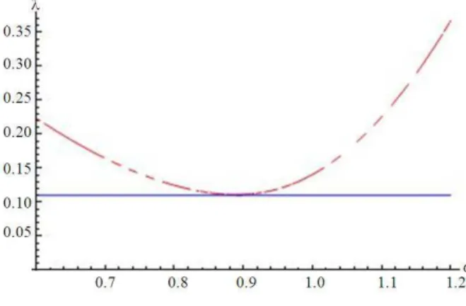
Fig. 1. The behviour of the spectral radius of the TSOR as a function of ω

1.0 0 0.25 0.25 1.0 0 1.0 0.25 0.25 1.5

A , b

0.25 0.25 1.0 0 0.5 0.25 0.25 0 1.0 1.0

−

   

   

   

=_{ } =_{ } − −

   

−

   

For simplicity we adapted the right hand side b as it was in Young (2003) and Youssef (2012) so that the exact solution is x1 = 1, x2 = 1, x3 = 1, x4 = 1.

It is well known that, for this system we have. The eigenvalues of the Jacobi iteration matrix TJ are the roots of the equation:

4 2

0.25 0.015625 0

µ + µ + =

The roots are:

1 2 0.353553I, 3 4 0.353553I

µ = µ = µ = µ = −

For the matrix, F 0.25 0.25 0.25 0.25

−

 

=_{− −} 

  the Singular

values are s1 = s2 = 0.353553.

It is clear that the Jacobi iteration matrix TJis a skew symmetric, accordingly their eigenvalues are pure imaginary complex numbers, and satisfies 2 2

i si

µ = .

3. RESULTS

• We used the SVD in proving the eigenvalue functional relation for the KSOR operator

• The minimization of the ℓ2-norm is used as a good estimation for determining the optimum value of the relaxation parameter in the KSOR method as well as in the SOR method

Fig. 2. The behaviour of the ℓ₂-norm of TSOR as a function of ω

Fig. 3. The behviour of the spectral radius of the TKSOR as a function of ω*

Fig. 4. The behaviour of the ℓ2-norm of TSOR as a function of ω* • From Fig. 1 and 2 we see that the calculated

• From Fig. 3 and 4 we see that the calculated results agree with our theoretical results

•

Numerical example illustrating and confirming the theoretical relations is considered

4. DISCUSION

Young (2003), considered the problem why convergence of the SOR method with the optimum ωopt in the sense of minimizing the spectral radius of the iteration matrix is some what slower than what might expected, the spectral radius is only an asymptotic measure of the rate of convergence of a linear iterative method. In his treatment Young (2003), established a relation between the eigenvalues of certain matrices related to A (the SOR iteration matrix, TSOR) and those of certain block 2×2 matrices.

Golub and Pillis (1990) raised the question of determining, for each k ≥ 1, a relaxation parameter ω∈(0, 2) which minimizes the Euclidean norm of the kth power of the SOR iteration matrix, associated with a real symmetric positive definite matrix with “property A”.

Hadjidimos and Neumann (1998), used the reduction of the SOR operator introduced by Golub and Pillis (1990), with the help of the SVD of the associated block Jacobi iteration matrix to obtain the minimizing relaxation parameter for the case k = 1. Yin and Yuan (2002), used the SVD to re-derive the eigenvalue functional relations for block skew symmetric matrices for the AOR method. Mill o et al. (2006), considered systems with block skew symmetric Jacobi iteration matrix and used the SVD in studying the behavior of the SOR operator from the ℓ₂-norm point of view they determined theoretically the minimizing relaxation parameter of the ℓ2-norm. Youssef (2012), defined the KSOR operator, we used the SVD in re-prove the functional eigenvalue relation for the KSOR operator and the corresponding unitary block 2×2 matrix ∆(ω*). we employed the same argument as in Yin and Yuan (2002), also in Mill o et al. (2006) for systems with block skew symmetric Jacobi iteration matrix and used the SVD in studying the behavior of the ℓ2-norm of the KSOR operator. We determined theoretically the minimizing relaxation parameter of the ℓ₂-norm for the KSOR operator. We confirmed our theoretical results by a numerical example. We will continue this study in a subsequent work in which we will consider a generalizations of the KSOR operator.

5. CONCLUSION

We used the same argument defined by Golub and Pillis (1990), used by Yin and Yuan (2002) also by Mill o et al. (2006), we proved that the KSOR iteration matrix TKSOR is unitary equivalent to a matrix ∆(ω*) having only 2×2 or 1×1 matrices on the diagonal. We minimize the ℓ_{2-norm of the KSOR operator for matrices}

whose Jacobi iteration matrix is skew symmetric. By our results, the optimal value of the relaxation parameter is:

*

opt 2

J 1 (p(T ))

ω = .

6. REFERENCES

Buckley, A., 1977. On the solution of certain skew symmetric linear systems. SIAM J. Numer. Anal., 1: 566-570. DOI:10.1137/0714035

Ehrlich, L.W., 1972. Coupled harmonic equations, SOR and Chebyshev acceleration. Math. Comput., 26: 335-343.

Golub, G.H. and J. Pillis, 1990. Towards an Effective Two-Parameter SOR Method. In: Iterative Methods for Large Linear Systems, Kincaid, D.R. (Eds.), Academic Press, New York, ISBN-10: 0124074758, pp: 107-119.

Hadjidimos, A. and M. Neumann, 1998. Euclidean norm minimization of the SOR operators. SIAM J. Matrix

Anal. Appl., 19: 191-204. DOI:

10.1137/S0895479896300498

Maleev, A.A., 2006. On the SOR method with overlapping subsystems. Comput. Math. Math. Phys., 46: 919-929. DOI: 10.1134/S0965542506060017

Milleo, I., J.H. Yin and J.Y. Yuan, 2006. Minimization of ℓ_{2-norms of SOR and MSOR operators. Comput.}

Applied Math., 192: 431-444. DOI: 10.1016/j.cam.2005.03.078

Woznicki, I. Z., 2001. On performance of SOR method for solving nonsymmetric linear systems. Comput. Applied Math., 137: 145-176. DOI: 10.1016/S0377-0427(00)00705-6

Yin, J.H. and J.Y. Yuan, 2002. Note on stationary iterative methods by SVD. Applied Math. Comput., 127: 327-333. DOI: 10.1016/S0096-3003(01)00010-8 Young, D.M., 2003. Iterative Solution of Large Linear Systems. 1st Edn., Dover Publications, Mineola, New York, ISBN-10: 0486425487, pp: 570.