A Work Project, presented as part of the requirements for the Award of a Master Degree in Economics from the NOVA – School of Business and Economics
LIKE MOTHER, LIKE SON? STUDYING THE
IMPACT OF MOTHERS’ SCHOOLING ON
CHILDREN’S YEARS OF EDUCATION IN MALAWI
Madalena Moniz Pereira Páscoa
783A project carried out under the supervision of Pedro Vicente January 6th, 2017
2 Abstract
Does a mother’s level of education impact that of her children? Motivated by gender disparities in Malawi’s educational landscape, this paper aims to answer this question through three identification strategies: with 2013 Malawi survey data, Ordinary Least Squares, Propensity Score Matching and Instrumental Variable methods are used to analyse the extent of the relationship between the education of women and that of their children. In the Instrumental Variable models, distance to secondary school is used as an instrument for mother’s years of education, resulting in an estimated impact of 0.314 years of education per additional year of mother’s education.
Keywords: education, women, instrumental variable, Malawi 1. Introduction
To classify education as a luxury would sound like an exaggeration to many. Not so much in countries with low levels of economic development, such as Malawi, where there is a noticeable male bias in educational attainment – for a lot of girls, access to schooling is not guaranteed. Even though Malawi may not be far from achieving gender parity in primary education, it is not uncommon for a girl to not go to school. In fact, large discrepancies start arising as soon as they hit the 4th year of primary school, with more girls than boys dropping out of school due to social principles and behaviours (in 2012, the proportion of individuals staying in school until 8th grade, the last year of primary education, was 53% for boys and 45% for girls).
With basis on the 2015 United Nations Human Development Report for Malawi, mean years of education for women are 3.4, contrasting with a 5.2 average for their male counterparts. This report also calculates the Gender Inequality Index (GII), which measures gender-based inequalities in three dimensions: economic activity, reproductive health and empowerment (including educational attainment in secondary and higher education by gender). In 2014, Malawi reached a GII of 0.611, which puts it in the 140th spot out of a 155-country analysis. Now, considering that this index can be interpreted as the loss in human development associated with inequality between female and male achievements in the three dimensions of GII, through this lens Malawi does not look especially progressive in regards to gender equality. In 2014, only 11.1% of adult women had 1: Malawi’s educational system is composed of 8 years of primary school followed by 4 years of secondary school.
3
completed secondary education, opposed to 21.6% of men. Within the long-term consequences of lower female education are high fertility, low economic growth and continued gender inequality in education: these can lead to a poverty trap, hence justifying the need for policy interventions geared towards educating girls2. But what else characterises Malawi’s educational system?
In Malawi, primary education was declared free in 1994. However, the educational system was under-resourced to begin with: schools were short of adequate classrooms, teachers and learning materials3. With the introduction of cost-free primary schooling came along an enrolment overflow, pushing the system to further resource exhaustion (e.g., the average class size in 2013 was 90 students4). If the system is overcrowded and the infrastructures are not up to par, the quality of education is more likely to be unsatisfactory – if parents can conclude this, they will be more likely to discard education, labelling it as an unhelpful investment. Furthermore, if the children are female, investing in their education may be deemed unnecessary altogether.
In line with this, our research ultimately intends to stimulate policy responses to gender disparity in education. More specifically, we will focus on the impact of women’s education on their children, attempting to measure the intergenerational impact of educating girls. Thus, the research question we will address is the following:
Does education of the mother impact education of the child, and if so, by how much? To answer this question, we will look at data from the 2013 Malawi Integrated Household Panel Survey, measuring education through years of education, for mothers as well as their children. This question is more complex than what meets the eye: a woman’s education can be the product of other more fundamental variables, that may themselves have a direct impact on a child’s education (for example, intrinsic ability of the mother) – for this reason, we have to be wary of possible
2: Klassen, Stephan. 2002. “Low Schooling for Girls, Slower Growth for All? Cross-Country Evidence on the Effect of Gender
Inequality in Education on Economic Development.” The World Bank Economic Review, 16(3): 345-373
3: Brossard, Mathieu, Diane Coury and Michael Mambo. 2010. “The Education System in Malawi.” World Bank Working Paper
no. 182
4
endogeneity, driven by omitted variable bias. Ergo, in pursuit of robustness, three identification strategies will be used: Ordinary Least Squares (OLS), Propensity Score Matching (PSM; assuming conditioning on observables) and Instrumental Variable (IV). For the last strategy, distance to secondary school will be used as an instrument for mother’s education; in order to have a good instrument, it needs to be correlated with the independent variable of interest, but uncorrelated with the residuals. Now, for distance to secondary school not to correlate with the errors from children’s years of education, we restrict the sample (5<age<14) for the IV specifications, only including individuals who are not yet of secondary school age and should not, consequently, be impacted by distance to secondary school. Even though it is a constitutional prescription, Malawi has yet to make primary schooling mandatory by law5 – this adds to the interest of studying the impact of mother’s education on her children’s (if primary schooling was mandatory, said impact might have been considerably smaller).
We find the following results: in the OLS model (unrestricted sample), we estimate that each extra year of education for the mother will have an impact of 0.102 additional years of education for her children. In one of our PSM settings (unrestricted sample), the years of education for a treated subject whose mother has completed primary education will be impacted by about 0.818. Finally, one of our IV specifications (restricted sample) estimates that each additional year of education for the mother will have an impact of 0.314 in her children’s years of education. By and by, we get statistically significant results that indicate the existence of a positive intergenerational effect caused by mothers’ education, lending yet more reasons for the implementation of policies steered towards educating girls.
The rest of the paper is organised as follows: in section 2, the existing literature on the subject is briefly reviewed; section 3 delves into the data used in this project, explaining its origins and
5: As described in the 2012 “Country Fact Sheet – Malawi”, developed by The Right to Education Project, which is supported
by ActionAid International, Amnesty International, Global Campaign for Education, Save the Children and Human Rights Watch.
5
sample design; section 4 is concerned with clarifying the estimation strategies used in this paper; in section 5, the empirical results are put forward, and these are later analysed in section 6, along with the project’s concluding remarks.
2. Literature
It is fairly common to assume that the educational level of parents has its toll on that of their children (Becker and Tomes, 1976; Black and Devereux, 2010) – after all, there is evidence that the setting in which a person is submerged during his/her first few years of existence has profound consequences on the rest of their lives (Heckman et al., 2015). However, there are several channels through which the intergenerational transmission of human capital can work – the archetypal dilemma between nature and nurture. The nature factor is related to the transmission of common genetic characteristics from parents to children, while nurture has to do with educated parents’ capacity to arrange for a better learning environment for their offspring (de Walque, 2005). In order to pinpoint the shape of this intergenerational link, three chief identification strategies are used: twins, adoptees and instrumental variables. In the twins’ methodology, the difference in education within pairs of identical twins is used to find effects on the schooling of their children (Behrman and Rosenzweig, 2002). Two identifying assumptions are at work here: one is that twin parents are identical in their inherited endowments (unobservable genetic effects, which cancel out) and the other is that twin parents are non-identical in years of schooling. Assuming that the difference between twin parents’ education is exogenous, results show that their children’s education is increased by 0.13 years per extra year of maternal schooling, with the impact of father’s education being close to double the size. Yet, since this approach demands that twins are almost, but not exactly, identical, it also raises the question of whether non-identical amounts of schooling between twins are randomly determined – if not, the school differences between twins
6
may be endogenously determined and lead to biased estimates (Bound and Solon, 1999). The second strategy is the comparison between natural and adopted children, another way to cancel out the genetically inherited impact. Here, each year of fathers’ schooling increases children’s education by 0.2 years, while mother’s schooling tends to have an insignificant effect on the schooling of adopted children. Even still, these types of estimation may be biased, as they assume that adopted children are randomly given for adoption and assigned to families (Chevalier, 2004). The third strategy is instrumental variable estimation, used to cope with the impossibility of randomly distributing parental education to assess its impact on children. One common technique is to instrument parental education through changes in the school leaving age (as seen in Black et al., 2003, and Oreopoulos et al., 2003), or through distance to school (Card, 1995, uses college proximity as an instrument for schooling). Studies on distance-to-university typically find a negative effect of distance on the probability of studying (Frenette, 2006 and Alm et al., 2009). In “Too Far to Go? Does Distance Determine Study Choices?”, the authors provide four theoretical reasons for the impact of distance on study behaviour: cost (direct, such as travel expenses and accommodation, and indirect, like opportunity costs), selection effects (individuals who are educationally disadvantaged tend to be from regions located far from universities), peer effects (based on the idea that similar parts of the community – academics, unskilled workers, etc. – live in similar locations, at similar distances from universities, hence influencing each other in regards to schooling choices) and local roots (oftentimes, when subjects are engulfed in a specific environment and there is no educational provision close by, they would rather not study than have to give up their surroundings in pursuit of education).
Pursuing gender equality in education should be a goal in and of itself, but it is in fact coupled with an inexhaustible amount of positive consequences. Evidence suggests that women’s schooling is
7
associated with social gains such as better child health (Currie and Moretti, 2003) and nutrition (Thomas et al., 1991), reduced infant mortality (Behrman et al., 1988), and improvements in children’s educational attainment (Rosezweig and Wolpin, 1994). Additionally, there is evidence of similar (if not larger) wage gains from education for women, with relatively higher returns to secondary schooling than men (Schultz, 2002). Educated women are less likely to work domestically, or in informal sectors, associated with lower income levels; rather, they are more likely to enter the formal labour market (Malhotra et al., 2003). Improvements in women’s education are also associated with faster economic growth: if the share of women with secondary education was increased by 1 percentage point, annual per capita income growth could be enhanced by 0.3 points on average, according to a study which encompasses 100 countries (Dollar and Gatti, 1999). Female schooling tends to have a greater impact than men’s schooling: when women’s education is 1 year above the average, the probability of children’s educational enrolment rises by 1 to 6 percentage points (Filmer, 2000).
3. Data
The data used in this paper comes from the 2013 Malawi Integrated Household Panel Survey (IHPS), conducted by the National Statistical Office (NSO) of Malawi and supported by an initiative carried out by the Development Research Group at the World Bank: the Living Standards Measurement Study – Integrated Surveys on Agriculture (LSMS-ISA)6.
The design of this survey follows the blueprint of other surveys under the LSMS scheme: a multi-topic, integrated household survey comprising household, agriculture and community questionnaires. The IHPS is, in fact, the follow-up to another survey conducted in 2010-2011, the IHS3 (Third Integrated Household Survey).
6: This project was financially supported by the Government of Malawi, Norway, the World Bank LSMS-ISA project, the
Department for International Development (DFID), Irish Aid, the Millennium Challenge Corporation (MCC), and the German Development Corporation (GTZ). None of these entities are responsible for the estimations and analyses reported here 7: There is no relevant variation in mothers’ education from one survey to the other – this is why we will not apply a difference-in-differences method.
8 3.1. Sample design
Keeping in mind that IHPS’s sample is engulfed in the design of the baseline sample (as IHPS is a subsample of IHS3, selected from its full sample systematically with equal probability), it is the sampling procedure for the IHS3 sample which should be outlined first. IHS3 used a stratified, two-stage sample design8, having based its frame on the listing information and cartography used in the 2008 Malawi Population and Housing Census (PHC).
First stage – selecting sample EAs: the primary sampling units (PSUs) are the census enumeration areas (EAs) used in the 2008 Population and Housing Census (PHC). Within each district, the sampling frame of EAs was sorted by urban/rural, administrative area and EA code, basing the size of each EA on the total number of households listed in the PHC. Then, sample EAs were selected systematically from the ordered list of EAs in the sampling frame (with probability proportional to size, due to the variability in the number of households per EA).
Second stage – selecting households: after constructing a listing of households per EA, 16 primary households and 5 replacement households were selected from the household listing for each EA. With IHPS (the sample of interest), the aim was to track and resurvey the baseline households in 2013, as well as the individuals that moved away from their baseline dwellings9 between 2010 and 2013. IHPS entails a total of 4000 households (of which 3104 are baseline households), with interviews having taken place between April and December 2013. IHPS’s sample was selected to be representative at the national, regional, urban and rural levels, and for six regional strata10. The sampling procedure for IHPS consisted in randomly selecting a sub-sample from IHS3’s sample enumeration areas (EAs): 204 out of 768 EAs were chosen to take part in IHPS (each EA with its corresponding households, chosen beforehand for IHS3). In order to guarantee reliable results for
8: A more detailed explanation of the sampling process for IHS3 can be found in “Malawi, Third Integrated Household Survey
(IHS3) 2010-2011, Basic Information Document” from the World Bank’s resources.
9: Seeing that they were not servants or guests during the first survey, were at least 12 years old and known to be living in
mainland Malawi, with the exception of those residing in Likoma Island or in institutions. Once one of these subjects was located, the new household that he/she joined since 2010 was also included in the IHPS sample.
10: Northern Region – Rural; Northern Region – Urban; Central Region – Rural; Central Region – Urban; Southern Region –
9
both urban and rural domains at the national level, the IHS3 sample EAs were post-stratified by urban and rural areas within each region. The distribution of the subsample of EAs and households ensures a minimum sample size for each region: e.g., a higher sampling rate is used for the urban stratum of each region, in order to improve the precision of panel estimates for urban territories. 4. Estimation strategy
The question we mean to address is whether a mother’s years of education impacts her child’s years of education. As the education of a mother can result from other more fundamental variables which may themselves directly impact a child’s education (e.g., the mother’s intrinsic ability), we have to be wary of possible endogeneity: it may hinder the analysis of the impact actually caused by mothers’ schooling, since there might be an omitted variable bias problem. To deal with it, and for the sake of robustness, we will run various types of regressions (assuming conditioning on observable variables) to investigate whether mothers’ schooling might have an impact on children’s years of education and, if so, by how much. During the course of this paper, some restrictions will be imposed – these are essential for our IV identification strategy, and imposed alongside unrestricted estimations in OLS and PSM, for the sake of comparability between methods:
mother location restriction: answers to the survey are given in 2013; to the extent that we wish for mother’s education to have been affected by the distance to secondary school (IV), we have to restrict our sample to the cases where the mother has lived in the same community for all of her life or has moved when she was still in school age (≤ 22 years old), so that the answer given in 2013 corresponds to the answer she would have given when she was still in school (to do this, we have to assume no government secondary schools were built/demolished in the communities). 5 < age < 14 restriction: this restriction means to confine our sample to those who are of primary school age (assuming no early starts or late finishes). This restriction is necessary for the estimation
10
of our IV models: since we are using distance to secondary school as an instrument, it cannot be related to years of education through any channel other than mother’s education. Hence, in order for distance to secondary school not to be correlated with the residuals in the years of education equation, we confine the sample to those who are not yet impacted by the distance to secondary school, as they are still in primary school age (older than 5 and younger than 14).
4.1. Ordinary Least Squares (OLS)
years of educationi = α + β1.mother’s educationi + β2.controlsi + εi (1) years of educationi = α + β1.mother’s educationi + β2.controlsi + β3.stratai + εi (2) Where subscript i stands for individual i, years of educationis the dependent variable, indicating the number of years of schooling attended by the individual (derived from the IHPS household survey question C08: “What was the highest class level you ever attended?”). Similarly, the independent variable of interest, mother’s education, points to the number of years of schooling attended by the individual’s mother, whereas controls stands for a vector of individual and community-level control variables (refer to Table 1 for a description of each variable). Finally, strata is a vector including dummy variables for each geographical stratum. The remaining specifications are similar to (2), except that they include additional restrictions or a dummy variable as the dependent variable of interest11: in (3), we include the mother location and the 5<age<14 restrictions, while in (4) we employ these restrictions alongside the substitution of mother’s education and father’s education by their respective parental education dummy.
Standard errors are clustered at the household level12, to account for intra-home correlation in errors.
11: Whenever mother’s education (the independent variable of interest) is represented as a dummy, so is father’s education (both
dummies are =1 if the mother/father has completed primary school).
12: We also experimented with clustering at the enumeration area level, with negligible differences in the levels of statistical
11 4.2. Propensity Score Matching (PSM)
years of educationi = α + β1.mother’s primary schooli + β2.controlsi + εi (5) using nearest neighbour(1) with replacement
In the PSM estimations, the treatment variable is mother’s primary school, a dummy variable =1 if the mother has completed primary school (assuming selection on observables). We use nearest neighbour and kernel procedures for matching. In nearest neighbour matching, an individual from the comparison group is chosen as a match for one (or more) in the treatment group, in terms of the closest propensity score. Kernel matching compares the outcome of each treated person to a weighted average of the outcomes of all untreated individuals, with the highest weight being placed on those with scores closest to the treated individual. The remaining specifications are: (6), using
age individual's age, in years
sex dummy variable =1 if individual is female
mother’s age individual's mother's age, in years
mother's sex dummy variable =1, as individual's mother is always female
married dummy variable =1 if individual is in a married or non-formal union
christian dummy variable =1 if individual is christian
muslim dummy variable =1 if individual is muslim
father’s education number of years of schooling attended by the individual’s father
father’s primary school dummy variable =1 if father has completed primary school
rural dummy variable =1 if individual resides in a rural area
poor dummy variable =1 if household’s 2013 total real annual
consumption per capita is below the absolute poverty line
home ownership dummy variable =1 if family owns home
household size number of people living in household as of 2013
piped water dummy variable =1 if the main source of drinking water is piped into dwelling or piped into yard/plot
employment measure dummy variable =1 if people in the community leave temporarily during certain times of the year to look for work elsewhere
north urban stratum dummy, =1 if individual lives in a North Urban region
north rural stratum dummy, =1 if individual lives in a North Rural region
centre urban stratum dummy, =1 if individual lives in a Centre Urban region
centre rural stratum dummy, =1 if individual lives in a Centre Rural region
south urban stratum dummy, =1 if individual lives in a South Urban region
south rural stratum dummy, =1 if individual lives in a South Rural region Table 1: control variables
12
nearest neighbour(1) with replacement and adding the strata controls; (7), using nearest neighbour(5) with replacement; (8), with a kernel matching method and, lastly, (9), which uses nearest neighbour(1) with replacement alongside the mother location and 5<age<14 restrictions (to allow for comparison between methods). In all PSM regressions (excluding kernel, where it is not applicable), Abadie-Imbens standard errors are used.
4.4. Instrumental Variable (IV)
years of educationi = α + β1.mother’s educationi + β2.controlsi + εi (10) with mother location and 5<age<14 restrictions
years of educationi = α + β1.mother’s educationi + β2.controlsi + β3.stratai + εi (11) with mother location and 5<age<14 restrictions
We will employ the mother location and the 5<age<14 restrictions in all of our IV specifications (the reason why is explained in the beginning of section 4), except for (12), where we remove the mother location restriction, so as to check whether we get a weaker instrument in that instance. If we intend to achieve validity in the IV estimations, the instrument will have to fulfil two requirements: to be related to the explanatory variable we want to instrument (mother’s education) and to be uncorrelated with the errors (ε). We propose to use distance to secondary school (the distance to the closest government secondary school, expressed in km), as an instrument for mother’s education, assuming it satisfies the two conditions stated above – distance to secondary school is strongly correlated with mother’s education, and likely to be uncorrelated with the residuals (since we will restrict our sample to those who are not yet old enough to be impacted by the distance to secondary school: 5<age<14 restriction). We will use Two-Stage Least Squares and run a weak instruments test for each specification.
13 5. Empirical results
We start by looking at descriptive characteristics for all the variables used in the regressions in Table 2. The average age of the respondents is 25.453, 51.4% of the sample is female and the mean distance to the closest government secondary school is 21.571 km. Moreover, about 74% of households are located in a rural area, whilst 34% of them are considered poor (i.e., the household’s 2013 total real annual consumption per capita is under the absolute poverty line). The average for years of education in the sample is of 5.243, with mother’s education having a slightly higher average value than father’s education; 23.1% of fathers and 20.3% of mothers have completed primary education.
variables observations mean standard error
years of education 16 293 5.243 3.986
mother's education, years 6 697 4.516 4.077
mother's primary school, dummy 6 734 0.203 0.402
age 16 464 25.453 17.088 sex 16 587 0.514 0.500 mother's age 6 661 33.649 18.015 mother's sex 6 734 0.628 0.483 married, dummy 16 467 0.382 0.486 christian, dummy 16 478 0.654 0.476 muslim, dummy 16 478 0.100 0.300
father's education, years 5 134 4.317 4.492
father's primary school, dummy 5 166 0.231 0.421
rural, dummy 16 587 0.739 0.439
poor, dummy 16 585 0.342 0.474
home ownership, dummy 16 587 0.767 0.423
household size 16 585 6.074 2.521
piped water, dummy 16 587 0.152 0.359
employment measure, dummy 16 587 0.640 0.480
distance to secondary school, km 15 785 21.571 24.845
north urban, dummy 16 585 0.246 0.430
north rural, dummy 16 587 0.000 0.000
centre urban, dummy 16 585 0.097 0.296
centre rural, dummy 16 585 0.276 0.447
south urban, dummy 16 585 0.107 0.309
south rural, dummy 16 585 0.274 0.446
Table 2: summary statistics
14 5.1. OLS
First, we make an assessment of the models’ performance by looking at their R²: in the first two specifications, the R² is close to 0.63, indicating that the model explains about 63% of the variation in years of education (52% for (3) and 51% for (4), where the mother location and 5<age<14 restrictions are imposed). As for age, the older a person is the more years of education he/she tends to have, while poor and rural lean towards a negative effect on years of schooling. As far as mother’s education is concerned, it is highly significant (at a 99% confidence level) in all specifications. Its coefficient is associated with the expected change in years of education for every additional year of mother’s education: in (1), where we estimate the model with just the individual and community level controls, there is statistical evidence that points towards a 0.105 years increase in years of education; (2), where we also include the geographical strata controls, estimates a 0.102 increase in years of education. In (3), we include the mother location and age restrictions, to make an OLS model that is comparable with the IV iterations, where these restrictions are necessary: we get evidence of a 0.053 increase in years of education per extra year of mother’s education. An additional year of mother’s education seems to have a smaller impact on those who are aged between 5 and 14 than on the unrestricted sample – it is possible that this effect is smaller for those in primary school age than for the population in general because primary school is meant to be mandatory in Malawi (even though this has not been enacted yet), making for a smaller toll of mother’s education on years of education. Finally, in (4), we use a dummy variable to be able to compare OLS with PSM models later on (as all PSM specifications use this variable as treatment): by using mother’s primary school, we are calculating the effect of a mother having at least 8 years of schooling; as such, its coefficient is expectedly larger than those of the other models: if mother’s primary school = 1, years of education tends to increase by 0.261.
15
(1) (2) (3) (4)
variables coef/se coef/se coef/se coef/se
mother's education, years 0.105*** 0.102*** 0.053***
-(0.014) (0.014) (0.012)
-mother's primary school, dummy - - - 0.261***
- - - (0.082) age 0.271*** 0.270*** 0.511*** 0.506*** (0.029) (0.029) (0.018) (0.018) sex 0.108* 0.108* 0.247*** 0.248*** (0.064) (0.064) (0.057) (0.058) mother's age 0.003 0.003 0.001 0.004 (0.003) (0.003) (0.003) (0.003) mother's sex -0.055 -0.055 -0.059 -0.020 (0.110) (0.110) (0.084) (0.079) married, dummy -1.366** -1.362** - -(0.546) (0.547) - -christian, dummy 2.190*** 2.185*** 0.151 0.176 (0.248) (0.246) (0.115) (0.116) muslim, dummy 1.236*** 1.220*** -0.710*** -0.730*** (0.300) (0.299) (0.232) (0.235)
father's education, years 0.093*** 0.091*** 0.042***
-(0.014) (0.014) (0.014)
-father's primary school, dummy - - - 0.377***
- - - (0.099)
rural, dummy -0.593*** -0.288* 0.017 -0.046
(0.108) (0.151) (0.149) (0.151)
poor, dummy -0.529*** -0.533*** -0.274*** -0.324***
(0.095) (0.094) (0.078) (0.076)
home ownership, dummy -0.074 -0.074 0.167 0.168
(0.112) (0.112) (0.116) (0.111)
household size 0.072*** 0.071*** 0.036** 0.033*
(0.025) (0.025) (0.018) (0.018)
piped water, dummy 0.678*** 0.706*** 0.576*** 0.555***
(0.148) (0.146) (0.149) (0.147)
employment measure -0.003 -0.029 0.084 0.065
(0.093) (0.092) (0.076) (0.077)
constant -1.181*** -1.431*** -3.177*** -2.837***
(0.302) (0.315) (0.253) (0.251)
stratum controls no yes yes yes
mother location restriction no no yes yes
5<age<14 restriction no no yes yes
parental education dummy no no no yes
number of observations 4 530 4 530 1 942 1 959
number of clusters 1 675 1 675 1 045 1 054
R² 0.630 0.632 0.521 0.513
Table 3: years of education // Ordinary Least Squares estimation
Note: strata dummies omitted (north urban, north rural, centre urban, centre rural, south urban, south rural). Standard errors - cluster corrected at the household level - reported in parentheses.
16 5.2. PSM
We start by looking at the logit regression used for calculating the p-score. Most variables for the calculation of the p-score show significance at the 1% level – the exceptions are sex, married, christian and rural13. Treatment =1 if the mother has completed primary school.
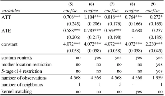
As far as the estimation results14 are concerned, in models (5) and (6) we use nearest neighbour (1) matching, with replacement. In (5), we get an ATT of 0.708 (on average, the treated subjects tend to have an extra 0.708 years of education if their mother has completed primary education, at a 99% confidence level) and an ATE of 0.588 (on average, a subject randomly drawn from the population would tend to have an extra 0.588 years of schooling if their mother had completed primary school).
13: Most of these refer to offspring’s characteristics, and what we want to estimate is the p-score for the mother’s primary school
completion; even still, we include these variables, as we intend to have homogeneity in controls throughout this study.
14: Where ATT: Average Treatment on the Treated; average impact of the treatment on those who participated
ATE: Average Treatment Effect on population: average impact of the treatment on the population ATU: Average Treatment Effect on the Untreated
ATE encompasses both ATT, the impact of a mother having at least 8 years of education on those who were treated (i.e., whose mother actually completed primary schooling), and ATU, the treatment effect that having a mother with primary education would have had on those who were not treated.
variables coefficient standard error
age -0.0175** 0.008 sex 0.062 0.064 mother's age 0.0433*** 0.003 mother's sex -1.210*** 0.078 married, dummy 0.473 0.375 christian, dummy -0.111 0.119 muslim, dummy -1.138*** 0.241
father's primary school, dummy 1.506*** 0.086
rural, dummy 0.153 0.113
poor, dummy -0.763*** 0.076
home ownership, dummy -0.431*** 0.080
household size -0.0327* 0.017
piped water, dummy 1.021*** 0.101
employment measure, dummy 0.398*** 0.070
constant -2.461*** 0.185
number of observations pseudo R²
Table 4: p-score for PSM //
logit estimation for mother's primary school
7 374 0.209
Note: strata dummies omitted. Propensity score applicable to models (6) through (9), since the propensity score for (5) is calculated without strata controls.
17
In (6), when we add the strata controls, we get a higher impact of mother’s primary school on those who were treated, at 1.104 (significant with 99% confidence), and an ATE of 0.783 (with 99% confidence). In (7), the model using nearest neighbour (5) with replacement, we get an ATT of 0.818 and an ATE of 0.769 (both with 99% confidence). Specification (8) uses kernel matching, with an estimated ATT of 0.764 (significant at 99% confidence) and an ATE of 0.680 (we do not know whether this result is significant, since the Stata command psmatch2 only reports standard errors for ATE when using Abadie-Imbens standard errors, which are not applicable in kernel matching). Both (7) and (8) have smaller ATTs and ATEs than (6), as well as smaller standard errors. Model (6) uses only one neighbour in the matching procedure; model (7) matches the treated subject with the 5 untreated subjects who are closest to him in terms of propensity score, whereas
(5) (6) (7) (8) (9)
variables coef/se coef/se coef/se coef/se coef/se
ATT 0.708*** 1.104*** 0.818*** 0.764*** 0.272* (0.245) (0.206) (0.176) (0.166) (0.165) ATE 0.588*** 0.783*** 0.769*** 0.680 0.237 (0.206) (0.217) (0.198) - (0.185) constant 4.072*** 4.072*** 4.072*** 4.072*** 2.230*** (0.058) (0.058) (0.058) (0.058) (0.045)
stratum controls no yes yes yes yes
mother location restriction no no no no yes
5<age<14 restriction no no no no yes
number of observations 4 568 4 568 4 568 4 568 1 959
number of neighbours 1 1 5 - 1
kernel matching no no no yes no
Table 5: years of education // Propensity Score Matching estimation
* significant at 10% // ** significant at 5% // *** significant at 1%
Note: Abadie-Imbens standard errors reported in parentheses for (5), (6), (7) and (9). Standard errors reported in parentheses for (8). Treatment variable mother's primary school is =1 when the subject's mother has completed primary school. Propensity score calculation with basis on age, sex, mother's age, mother's sex, married, christian, muslim, father's primary school dummy, rural, poor, home ownership, household size, piped water, employment measure, north rural, north urban, centre rural, centre urban, south rural and south urban variables (except for (5), whose propensity score does not account for the strata controls).
18
(8) uses kernel matching, comparing the outcome of each treated person to a weighted average of the outcomes of all untreated individuals. In comparison with nearest neighbour (1), for both nearest neighbour (5) and kernel matching there is a trade-off between the possibility of increasing bias and achieving smaller variance – hence the smaller values for ATT and ATE in (7) and (8). In model (9), we add the mother location and 5<age<14 restrictions, to compare PSM results with the IV specifications later on. With the restricted sample, we find an ATT of 0.272 (with 90% confidence) and an ATE of 0.237 (nonetheless, this result is not significant): thus, estimates suggest that, on average, a treated subject tends to have an extra 0.272 years of education if their mother has completed primary education.
5.3. IV
mother's education, years coefficient standard error P>|t|
distance to secondary school, km -0.016 0.004 0.000
age -0.163 0.044 0.000
sex 0.044 0.143 0.755
mother's age 0.081 0.006 0.000
mother's sex -1.890 0.259 0.000
married, dummy 0.000 (omitted)
-christian, dummy 0.246 0.240 0.305
muslim, dummy -0.157 0.459 0.733
father's education, years 0.232 0.033 0.000
rural, dummy 0.032 0.427 0.941
poor, dummy -0.427 0.220 0.052
home ownership, dummy -0.077 0.329 0.814
household size -0.143 0.052 0.005
piped water, dummy 1.106 0.478 0.021
employment measure, dummy 0.297 0.221 0.179
constant 4.371 0.685 0.000
number of observations number of clusters
Kleibergen-Paap F-statistic
Table 6: 2SLS // first stage regression for mother's education
1850 991 14.235
Note: first stage regression of the variable to be instrumented (mother's education ) on the controls and the instrumental variable (distance to secondary school ). Standard errors are clustered at the household level.
19
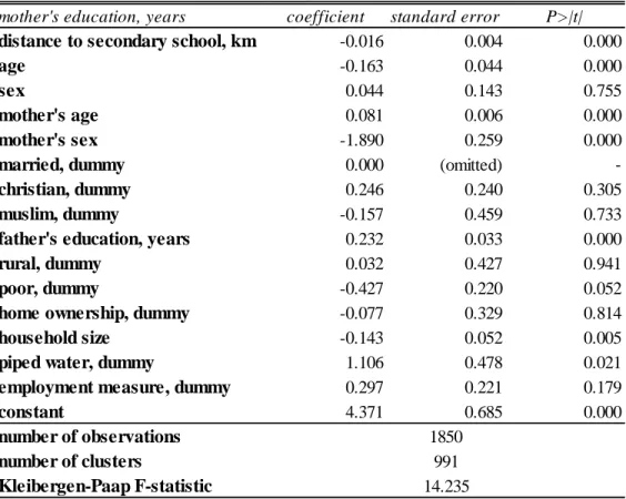
In the first stage for model (11), we regress the variable to be instrumented (mother’s education) on the controls and the instrumental variable (distance to secondary school). The Kleibergen-Paap F-statistic is used to test for weak instruments and is robust when there is clustering of the standard errors. In order to have a good instrument, we want this F-statistic to be higher than 10, which is the case here15 (F-stat = 14.235) – this means we can reject the hypothesis of distance to secondary school being a weak instrument. From here on out, we will assume that we have a valid instrument (except for specification (12), which we will address later).
In (10), where only the individual and community level controls are included, the estimated return to one additional year of mother’s education is 0.309 years of schooling, at a 95% confidence level. The coefficient for (2), where we also account for the geographical controls, is slightly higher, at 0.314; also, this specification has a higher Kleibergen-Paap F-statistic (indicating a stronger first stage) as well as a more significant coefficient (with 99% confidence). If we remove the mother location restriction, as is done in iteration (3), we get a coefficient that is smaller (0.296) than we would get otherwise. Removing this restriction leads to including in the sample individuals whose mothers lived in different communities during school age – thus, for those cases, the information about the distance to a government secondary school (the instrumental variable), as measured in 2013, will have no relationship with mother’s education. This is why iteration (12) presents the weakest first stage of all variations (i.e., the smallest F-statistic, at 9.823, rendering the instrument weak), hence justifying the use of the mother location restriction.
Comparing estimation methods
Before proceeding with comparisons, there is a difference between these OLS, PSM and IV models’ results that we should consider– while the results for OLS and PSM are Average Treatment Effects (ATE, i.e. the average impact on the population), the results for IV are Local Average
20
(10) (11) (12)
variables coef/se coef/se coef/se
mother's education, years 0.309** 0.314*** 0.296** (0.123) (0.118) (0.125) age 0.568*** 0.568*** 0.567*** (0.032) (0.030) (0.025) sex 0.231*** 0.227*** 0.250*** (0.069) (0.069) (0.059) mother's age -0.020* -0.020** -0.016* (0.010) (0.010) (0.009) mother's sex 0.415 0.433* 0.521* (0.267) (0.247) (0.316)
married, dummy (dropped) (dropped) (dropped)
- -
-christian, dummy -0.012 0.003 0.124
(0.143) (0.133) (0.116)
muslim, dummy -0.684** -0.744*** -0.772***
(0.271) (0.266) (0.260) father's education, years -0.020 -0.020 -0.017 (0.037) (0.033) (0.038)
rural, dummy -0.135 0.080 0.098
(0.195) (0.199) (0.141)
poor, dummy -0.159 -0.146 -0.121
(0.112) (0.119) (0.126)
home ownership, dummy 0.208 0.207 0.264**
(0.143) (0.141) (0.123)
household size 0.066** 0.068** 0.067**
(0.027) (0.029) (0.031)
piped water, dummy 0.323 0.292 0.336
(0.245) (0.229) (0.243)
employment measure, dummy 0.023 -0.000 0.008
(0.116) (0.110) (0.093) constant -4.503*** -4.646*** -4.843*** (0.691) (0.572) (0.680) number of observations 1 850 1 850 2 518 number of clusters 991 991.000 1 358 Kleibergen-Paap F-statistic 11.911 14.235 9.823 centered R² 0.315 0.310 0.371
Table 7: years of education // Instrumental Variable estimation
Note: strata dummies omitted from table (north urban, north rural, centre urban, centre rural, south urban and south rural). Standard errors - cluster corrected at the household level - reported in parentheses.
21
Treatment Effects (LATE, i.e. the average impact for an instrument specific subpopulation – the people who are induced into treatment by the instrumental variable). Since we are not sure whether the assumption of a homogeneous treatment effect holds (i.e., that the effect of the program is the same for the population as it is for the instrument specific subpopulation), LATE will typically differ from ATE16.
OLS and PSM: OLS model (4) is the one we can compare with the PSM variations, as it is the only OLS regression which uses a dummy as independent variable of interest. As it employs the mother location and 5<age<14 restrictions, we will compare it with the PSM variation that does so too: model (9). The coefficient associated with mother’s primary school in (4) is 0.261 (with 99% confidence), slightly smaller than the ATT from model (9), which is 0.272 (with 90% confidence)17. With similar results, these models point towards a positive impact of mother’s primary school completion on her children’s years of education.
OLS and IV: In (3), the OLS model comparable with IV, one extra year of mother’s education is estimated to have an impact of 0.053 on an individual randomly drawn from the population (ATE with 99% confidence); as for (11), one of the IV models, an extra year of mother’s education is estimated to have an impact of 0.314 additional years of education for her child for the instrument specific subpopulation (with 99% confidence). With the IV estimation method, we get higher coefficient estimates of the impact of mother’s education than we get with OLS, but we do so because IV estimates the impact of mother’s education on the individuals who are induced into treatment due to distance to secondary school, the instrumental variable (so IV’s LATE is higher than OLS’s ATE). IV estimates are also higher than OLS’s at the cost of a larger standard error: 0.012 in OLS versus 0.118 in IV.
16: LATE estimates are still interesting to our case, as they reflect the impact of mother’s education on those who were induced
into treatment due to the distance to secondary school (the instrument) – this may be a push forward for policies aimed at increasing schooling through reduced distance to school.
17: The coefficient for OLS model (4) is, however, slightly higher than the ATE for PSM model (9), which is 0.237 – however,
22 PSM and IV: in PSM model (9), a mother having completed primary school has an estimated impact of 0.272 additional years of education for children who were treated (ATT with 90% confidence, as the ATE of 0.237 is not statistically significant). The coefficient estimated through PSM is slightly lower than the one estimated through IV, which is 0.314: this difference may be due to the IV coefficient being a LATE, reflecting the effect of mother’s education on the share of the population that is induced into treatment by the instrumental variable – since the assumption of a homogeneous treatment effect is uncertain, IV’s results will normally contrast with PSM’s. When comparing IV models to OLS and PSM specifications, we see that the LATE (0.314) tends to be higher than the ATE (0.053 in OLS and 0.237 in PSM, although not significant). The presence of endogeneity in the OLS model could be a factor, but any correlation between mother’s education and the error term is expected to be positive (due to an upwards ability bias), hence not justifying the higher values of the IV estimations. To help explain this difference between IV and OLS results, we can make a parallel with the literature about returns to education18.According to Card (1999), the coefficients for IV estimations based on innovations in the school system tend to be higher than OLS’s: a possible explanation is that the marginal returns to education for some population subgroups (especially those whose schooling decisions are most affected by innovations in the school system) are higher than the average marginal returns to education in the population. In this case, IV estimates are expected to be higher than OLS’s.
6. Concluding remarks
Throughout this paper, we have studied the impact of mothers’ years of education on children’s years of education, using 2013 Malawi survey data. Due to endogeneity concerns (the possibility of omitted variable bias), we have assumed conditioning on observables for estimating the OLS and PSM models; as a further defense against possible endogeneity, we have also conducted IV 18: Which instruments the education variable, as is done here. This should be done with due caution, as we are dealing with a
different dependent variable here – years of education. Even still, looking at some returns to education references may help to explain why the IV coefficients are greater than the OLS ones, apart from the expected difference between LATE and ATE estimates.
23
estimations. In all of the variations performed19, mother’s education was deemed to have a significant impact on the years of education of children. In (2), one of the OLS models without restrictions, the estimated impact of mother’s education on years of education is 0.102. In PSM model (6), a treated subject whose mother has completed primary education will see his years of education increase by about 1.104. In IV specification (11), we estimate that each additional year of mother’s education has an impact of 0.314 in her children’s years of education20.
Nonetheless, this paper has some limitations. If the decision associated with mother’s primary school is not solely based on observable characteristics, the results for the OLS and PSM models may be biased. Additionally, due to the nature of the available data, only one instrumental variable was used (having access to more instrumental variables would have allowed for an overidentification test, to check whether the excluded instruments are independent from the residuals), and it requires restrictions regarding age and mother’s location, limiting this study’s external validity. Thus, it would be desirable to further investigate the usage of distance to secondary school as instrumental variable, but doing so with a sample that includes data on the distance to secondary school for all mothers at the time of schooling21.
All in all, this paper delivers statistical evidence on the ripple effect that mother’s schooling can have on the schooling of her children, encouraging us to stimulate and develop policies towards the improvement of women’s education. In the long-term, Malawi’s gap between the education of women and men can have consequences like high fertility and low economic growth. These may sow the seeds for a poverty trap, thereupon justifying the need for the development and application of policies geared towards educating girls. If we mean to reduce education gaps, we must address the barriers to accessing education: poverty (by and large, if the family has limited funds and has to choose whom to send to school, it might be more inclined to choose boys), early pregnancies, 19: The exception being the ATE for PSM model (9).
20: For an instrument specific subpopulation.
21: Since this is not available, IV estimations in this paper have to abide by the mother location restriction, which requires for a
mother to have lived in the same location throughout her life, or to have changed when she was still of school age (≤ 22 years old).
24
adverse cultural practices (women are more commonly required to stay at home, be it to care for family members or to take care of house chores) or distance to school – possible topics for further studies. Possible solutions are building more schools in remote areas, or interventions on the demand-side: cash transfers conditional on school attendance have proven to be effective in similar situations (e.g., in Mexico).
At the end of the day, vouching for women’s schooling is vouching for educating the next generation, ensuring that the values of universal education and gender equality continue on through time.
References
Abadie, Alberto and Guido Imbens. 2009. “Matching on the Estimated Propensity Score.” NBER Working Paper no. 15301.
Alm, James, and John V. Winters. 2009. "Distance and intrastate college student migration." Economics of Education Review, 28(6): 728-738.
Becker, Gary S. and Nigel Tomes.1976. "Child Endowments, and the Quantity of Children." Journal of Political Economy, 84(4): 143-162.
Behrman, Jere R. and Mark R. Rosenzweig. 2002. “Does Increasing Women’s Schooling Raise the Schooling of the Next Generation?” American Economic Review, 92(1): 323-334
Behrman, Jere R., Anil B. Deolalikar and Barbara L. Wolfe. 1988. “Nutrients: Impacts and Determinants.” The World Bank Economic Review, 2(3): 299-320
Black, Sandra E. and Paul J. Devereux. 2010. “Recent Developments in Intergenerational Mobility” IZA Discussion Papers, no. 4866.
Black, Sandra E., Paul J. Devereux and Kjell G. Salvanes. 2005. “Why the Apple Doesn't Fall Far: Understanding Intergenerational Transmission of Human Capital” American Economic Review, 95(1): 437-449
Bound, John and Gary Solon. 1999. “Double Trouble: On the Value of Twins-Based Estimation of the Return to Schooling” Economics of Education Review, 18(2): 169-182
Caliendo, Marco and Sabine Kopeinig. 2005. “Some Practical Guidance for the Implementation of Propensity Score Matching” IZA Discussion Papers, no. 1588.
Card, David. 1993. “Using geographic variation in college proximity to estimate the return to schooling.” National Bureau of Economic Research, no. w4483.
Card, David. 1999. "The causal effect of education on earnings." Handbook of Labor Economics, 3: 1801-1863.
Card, David. 2001. "Estimating the return to schooling: Progress on some persistent econometric problems." Econometrica, 69(5): 1127-1160.
Chevalier, Arnaud, Colm Harmon, Vincent O’ Sullivan and Ian Walker. 2013. “The impact of parental income and education on the schooling of their children” IZA Journal of Labour Economics, 2:8.
25
Chevalier, Arnaud. 2004. “Parental Education and Child’s Education: A Natural Experiment” IZA Discussion Papers, no. 1153.
Currie, Janet and Enrico Moretti. 2003. "Mother's Education and the Intergenerational Transmission of Human Capital: Evidence from College Openings." Quarterly Journal of Economics VCXVIII, 4: 1495-1532
de Walque, Damien. 2005. “Parental Education and Children’s Schooling Outcomes: Is the Effect Nature, Nurture, or Both? Evidence from Recomposed Families in Rwanda” World Bank Policy Research Working Paper, no. 3483
Denzler, Stefan and Stefan C. Wolter. 2011. “Too Far to Go? Does Distance Determine Study Choices?" IZA Discussion Papers, no. 5712.
Dollar, David and Roberta Gatti. 1999. “Gender Inequality, Income, and Growth: Are Good Times Good for Women?” World Bank Policy Research Report on Gender and Development, Working Paper Series, 1: 2-22.
Elango, Sneha, Jorge Luis García, James J. Heckman and Andrés Hojman. 2015. “Early Childhood Education” NBER Working Paper Series, no. 21766.
Filmer, Deon. 2000. “The Structure of Social Disparities in Education: Gender and Wealth.” Policy Research Working Paper no. 2268.
Frenette, Marc. 2006. “Too far to go on? Distance to school and university participation.” Education Economics, 14(1): 31-58.
Holmlund, Helena, Mikael Lindahl and Erik Plug. 2011. "The Causal Effect of Parents' Schooling on Children's Schooling: A Comparison of Estimation Methods." Journal of Economic Literature, 49(3): 615-51.
Klassen, Stephan. 2002. “Low Schooling for Girls, Slower Growth for All? Cross-Country Evidence on the Effect of Gender Inequality in Education on Economic Development.” The World Bank Economic Review, 16(3): 345-373
Kling, Jeffrey R.. 2001. "Interpreting instrumental variables estimates of the returns to schooling." Journal of Business & Economic Statistics 19(3): 358-364.
Malhotra, Yogesh. 2003. “Measuring Knowledge Assets of a Nation: Knowledge Systems for Development” Report of the Ad Hoc Expert Group Meeting on Knowledge Systems for Development, Department of Economic and Social Affairs Division for Public Administration and Development Management, United Nations: 68-126
Oreopoulos, Philip, Marianne E. Page and Ann Huff Stevens. 2006. "The Intergenerational Effects Of Compulsory Schooling" Journal of Labor Economics, 24: 729-760
Pande, Rohini, Anju Malhotra and Caren Grown. 2003. “Impact of Investments in Female Education on Gender Equality” International Center for Research on Women: 2-37.
Rosenzweig, Mark R. and Kenneth I. Wolpin. 1994. “Are There Increasing Returns to the Intergenerational Production of Human Capital? Maternal Schooling and Child Intellectual Achievement.” Journal of Human Resources, 29(2): 670-693.
Schultz, T. Paul. 2002. “Why Governments Should Invest More to Educate Girls” World Development, 30(2): 207-225.
Staiger, Douglas and James Stock. 1997. “Instrumental Variables Regression with Weak Instruments.” Econometrica, 65(3): 557-586.
Thomas, Duncan, John Strauss and Maria-Helena Henriques. 1991. “How Does Mother's Education Affect Child Height?” The Journal of Human Resources, 26(2): 183-211