A Work Project, presented as part of the requirements for the Award of a Double Degree in Economics from NOVA School of Business and Economics and Maastricht School of Business and
Economics
THE GRADUATE:
Spillovers From The Entry of The First Worker With a College Degree in
a Firm
João Prestes Sousa Korrodi Ritto, 623
A project carried out under the supervision of Professor Pedro Portugal and the co-supervision of
Professor Trudie Schills
THE GRADUATE:
Spillovers from the Entry of the First Worker with a College
Degree in a Firm
January 7, 2015
Abstract
In this thesis a large panel of data on Portuguese workers is used to estimate the effect of the
entry of the first graduate in a firm in his colleagues’ productivity. Propensity Score Matching is
the methodology used and robustness tests are also presented to reinforce the credibility of the
results. A spillover of approximately 5.10% is found, which means that the hiring of the first
college graduate is an important stage in the development of a firm which benefits all workers. It
is also shown that small firms benefit more from the entry of the first college graduate, specifically,
I. Introduction
The last years have seen a growth in the field of Labor Economics with different topics regarding education, job training and wages, among others, receiving a lot of attention. While it seems now to be consensual that education has a positive effect on a worker’s wage, there is less discussion and consensuality on whether the education of a worker also benefits his co-workers. The idea that a worker’s education or performance may affect his colleagues is not a new one, however. Models of Macroeconomics, for example, have incorporated this idea of positive externalities from human capital since the Lucas Model (1988).
The relevance of this question is of the utmost importance for our understanding of a society’s development and also for public policy matters. The existence of a positive externality of education would justify Government’s subsidization of public education, which is more difficult to justify if education only benefits the individual who takes it. Furthermore, this kind of understanding would also be useful to understand the mechanics of growth in developed countries.
This thesis attempts to give a response to the question: "does the first graduate increase the productivity of his colleagues in the firm?". While very specific, this question addresses an essential issue of whether college education brings some kind of benefit to the productivity of a firm. A college graduate has gone through a process of education which is more specialized in an area and has learned in an environment much more challenging than the one provided by secondary school. It is interesting to see if this has strong effects, both from an Economics of Education perspective and a Labor Economics perspective.
A large panel of data is used to estimate spillovers through the method of the propensity score matching. This differentiates this thesis from any other paper on firm-level spillovers, given that these always use a simple panel regression and do not look specifically at the first graduate hiring but rather at the average level of education. The advantage of using matching is that we are taking into consideration the fact that the firms that hire may not be easily comparable to the ones that do not, so we try to find firms that are comparable, instead of trying to compare different things. The results found, because of this, are also quite different from the existent literature, however, I believe they are also more credible. I try to control for all relevant variables that could cause bias.
productivity of his colleagues during the first year. As intuition would predict, I show that smaller firms have a higher spillover from human capital.
This thesis continues as follows. The next section provides a comprehensive description of the literature that already exists on this topic. Section III discusses a little bit of the theory that is behind the analysis in order to help understand the choices made in the estimation. This is complemented by section IV which discusses the methodology used, matching. Section V analyses the data that was used and Section VI presents and discusses the results. In Section VII additional results on the effect of the second graduate are presented. Section VIII concludes and suggests the direction for further research.
II. Literature Review
Since the advent of Labour Economics, many studies have been interested in finding the relationship between education and productivity, or education and wages. The question of whether schooling has inherent value in itself rose to proeminence with the battle between the rival theories of Human Capital theory of education supported by economists such as Becker and the signalling theory of education advanced in Spence (1973). The difference between these two theories is that the former argues that education raises productivity and has inherent value in itself while the latter states that education serves only as a tool to signal more able workers and does not really increase productivity in itself. The difficulty in estimating the real effects of education are in the possible and probable correlation between education and ability which is not measurable. Some papers have managed to overcome this problem in a convincing way, like Angrist and Krueger (1991)1 who taking into consideration compulsory schooling laws use date of birth as an instrumental variable and find a return of educationof 7.3%; Ashenfelter and Krueger (1994) who use data of identical twins to isolate the effect of schooling from the ability level and find an estimate of 12-16% increase in wages per year of education; Card (1995) who uses geographical proximity to college and finds a return of 10-14% per year of education. The present thesis however, concerns itself with the importance of education to productivity, but not in a similar fashion. It looks at the effects of education on the productivity of the workers’ colleagues or fellow citizens. These externalities are termed spillover effects.
The idea that education may have these kind of external effects comes already from Alfred
Mar-1
shall’s Principles of Economics first published in 1890. There is however, many different channels through which they can appear. Acemoglu and Angrist (2000) provide a clear explanation of the dis-tinction between nonpecuniary and pecuniary external effects of education. The former work through the exchange of ideas and learning by doing that can occur in the contact between workers. Contrarily, the latter works through the price mechanism or through the accumulation of capital, that may occur as a consequence of the complementarity of educated workers and physical capital, which can also benefit non-educated workers. Acemoglu (1996) gives a model for education spillovers at the city level in which, simultaneously, firms have to choose their physical capital level and workers have to choose their human capital. Matching in the labor market has some degree of randomness, which means that higher physical capital firms will not be able to get the higher educated workers with certainty. The equilibrium of this model is one in which all firms invest in the same level of physical capital which is dependent on the whole level of human capital of the city, therefore if a group of workers increases their human capital level, firms will increase their physical capital and some of the workers who did not increase their education will also benefit from this higher level of physical capital. Some studies do confirm this idea that physical capital has a higher complementarity effect the higher the education of workers. Bartel and Lichtenberg (1987), for example, find evidence of a comparative advantage of educated workers in implementing new technologies, while Griliches (1969) estimates parameters for a production fuction finding evidence of higher complementarity between capital and skilled workers than with unskilled workers.
an increase in the average level of education at low levels, like high school, will not produce spillovers, the increase in the share of college graduates will. Indeed this theory is reconcilable with the fact that Acemoglu and Angrist, as well as Rudd, do not find spillovers effects, whereas Moretti finds an effect between 6% and 7% for an increase of 10p.p. in the share of college graduates, as the former use average years of education while the latter uses share of college graduates.
Another important contribution to the literature was given by Ciccone and Peri (2006). They show that estimating spillover effects with a Mincer equation will provide results that are biased upwards in a very significant way. Using a calibrated model that they create, they find that the Mincerian Approach may find a spillover of around 8 percent when in fact there is no spillover in the model by construction. The reason for this has to do with the general equilibrium effects in wages caused by increases in the number of educated workers and consequent decrease of uneducated.
The present thesis, contrarily to the literature thus far discussed, estimates spillovers at the firm-level instead of at the city or state firm-level. The literature which takes this approach is far less vast. In all likelihood there is more than one reason for this. To start with, endogeneity issues may be present -as will be discussed later - which have made some researchers stay away from the topic. Secondly, and perhaps more important, is that even if these spillover effects exist, they will obviously be much smaller than the effect of education on one’s wage and because of that it is a topic less appealing to researchers. Despite this, there is some literature around this subject. There is a set of papers which look at peer effects at a workplace level - examples of which are Falk and Ichino (2006), Mas and Moretti (2009) and Guryan et al. (2009). Again, contradicting results are found. Guryan et al. (2009), nevertheless, argue that the different results can be conceivable in the light of the different workplace environments that each paper uses in its research. These authors discuss that possibly productivity peer effects occur at menial tasks but not in those jobs that require a lot of talent or knowledge. This would, then, explain why Mas and Moretti (2009) find significant peer effects in the job of supermarket cashier and Falk and Ichino (2006) in a simple job of folding letters and stuffing them into envelopes whereas Guryan et al. (2009) fail to find any significant effects in professional golfing.
college graduates instead of average level of education, as well as the difference of empirical strategy. While we look at the entry of the first college graduate to estimate a spillover of this particular event, Martins simply tries to access the effect of average education on wages in the stock of workers. We believe that looking at data for the entry of workers in a firm is much more trustworthy than looking at data from a stock of workers and trying to find spillovers. Battu et al. (2003) and Metcalfe and Sloane (2007) also look at education spillovers at a firm level in the UK, both finding spillovers around 11% per year of education. This value is huge, above the value that they find for the return of own education. A problem of ommited variable bias is likely to be present though. The authors do not take into consideration the possibility that the choice of a firm to hire workers more educated may be correlated to factors that increase wages by themselves.
III. A Discussion about Spillovers
As discussed in the Literature Review there is already some research on the area of spillovers of education. Nevertheless, most of these studies take a different or broader focus than this thesis. The main interest of this thesis is a very specific one - to find out whether there are significant positive spillovers from the entry of the first college graduate in a firm. The idea underlying this is that this first college graduate brings in new knowledge which can benefit other workers. Obviously, there is no reason to believe that the first college graduate is the only one that brings benefits to the firm, it is even possible that a second one brings higher spillovers by a mechanism of complementarity between both graduates. Despite this possibility, we still start by looking at the first graduate because of two reasons. To begin with, this feels like the right place to start the research, the impact of the first college graduate, not the second or the third, etc. Secondly, looking at the entry of additional graduates creates additional complications. Say that the second graduate joins right after the first, it may be hard to detach both effects from each other, especially if we do not expect the two spillovers to take the same time to act. That being said, in Section VII we take a brief look at the effects of the entry of other graduates besides the first, leaving, nevertheless, room for further research.
such as share of knowledge, would be permanent because learning is a process that once completed does not depend on the presence of the graduate, nevertheless, peer effects, which also look as a reasonable hypothesis, would disappear once the graduate leaves because workers no longer feel social shame for being less productive. This is a relevant point because if we look for an effect that happens two years after the entry of the graduate we need to know whether we should look for spillovers if the graduate has already left. I decide to look at effects of the first type, based on the share of knowledge. This means that the effects would be permanent. Jovanovic and Rob (1989) create a model for "the growth and diffusion of knowledge".2 This also takes us to another point that must be discussed, the lag of the effect.
We need to find out how many years after we should expect the effect to appear. This is not considered in other papers of this type.3 In the methodology used in this paper, matching, which is
discussed in the next section, this becomes important to get the adequate results, as will be explained. Again, theory does not really tell us much on this. Different empirical frameworks must be tested to find out which one more accurately describes the behavior of the data.
Another issue in this thesis is the desire to estimate changes in productivity. Data on individual productivity is very rarely available. To begin with, most databases are not collected from the firms themselves, the only entity which could possibly have information on which part of the production is attributable to each worker. Secondly, most of the time this information is not possessed by even firms themselves because of a difficulty in observability. This thesis, then, bases itself on the assumption that there is no strong market power by firms and so increases in productivity can be collected by workers in wages. Wages can, then, be used as a measure of productivity. Before proceeding, let us analyze the consequences of this assumption. If a market is perfectly competitive, indeed, all productivity gains will be reflected in the wage, but if, on the opposite end, it is monopsonistic, any increases in productivity of a worker will be appropriated by the firm and no increase in wages will, thus, occur. If there is some degree of market power of the firms (monopsonistic competition) in the labor market which is less extreme than monopsony we will get a middle-of-the-way situation, in which workers receive part of their productivity increase in wages and another part is appropriated by the firm. Formally:
△w= (1−M)× △P
2
The reference to this paper has the sole objective of providing the reader with the information of where to find a theoretical model for the share of knowledge and how these mechanisms can be modelled. The model itself is not in anyway relevant for the understanding of the empirical framework of this paper.
3
Where M is a measure of the market power of the firms, M = 1 for monopsony andM = 0 for perfectly competitive labor markets. Under these conditions, it can be stated that by using wages I will be finding a lower bound on spillovers. To see this:
△w=α⇔(1−M)× △P =α⇔ △P = α
1−M ⇔ △P ≥α. The key for the last step is the fact thatM ∈[0,1].
This result tells us that if we find spillovers, then we can be certain of its existence, however if we do not, that could be an effect of the existence of strong market power and we cannot conclude with certainty that no spillovers are present.
IV. Methodology
The methodology which I use to estimate the presence or absence of spillovers is matching. The idea is to consider the entry of the first graduate as a "treatment" that will increase the productivity of the other workers of the firm. While matching does not, in itself, eliminate the possibility of hidden bias it presents significant advantages to a standard regression approach. To begin with, unlike regression analysis, matching will allow us to look for the spillover effects without making any restrictive assumptions on the functional form. In a multiple regression one must necessarily assume that the independent variables affect the outcome, in a specific way, most of the times linearly. Matching does not require this. Secondly, given that the hiring of the first graduate by a firm is not really random, a matching estimator is more convicing to try to overcome this issue by focusing on the common support (I explain the common support concept below).
The idea of matching is to compare two firms in the same conditions in which only one has hired its first graduate. By doing this comparison, we expect to find an effect in the wages of this firm which we can attribute to the entry of the college graduate. The first relevant question is on which covariates to do the matching, that is, what variables do we require to be similar so that we can consider the firms comparable? Theoretically, matching should be done on those covariates that affect both the independent variable (wages) and the probability of having been treated (probability that the firm would hire its first college graduate). This means that in our example we need to match on firm’s characteristics that look relevant for the hiring of a college graduate. This is likely to include the education and tenure of its workers, the size, the percentage of males, among others.
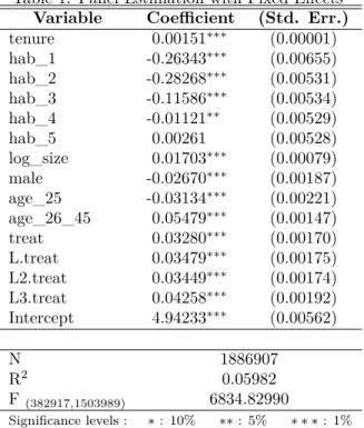
the effects of the hiring. There is no good theoretical answer for this and to get an idea of how to proceed I run a preliminary panel data regression with fixed effects, with dummies for the year of the hiring, one year after, two years after and three years after.
Table 1: Panel Estimation with Fixed Effects
Variable Coefficient (Std. Err.)
tenure 0.00151∗∗∗
(0.00001)
hab_1 -0.26343∗∗∗
(0.00655)
hab_2 -0.28268∗∗∗
(0.00531)
hab_3 -0.11586∗∗∗
(0.00534)
hab_4 -0.01121∗∗
(0.00529)
hab_5 0.00261 (0.00528)
log_size 0.01703∗∗∗ (0.00079)
male -0.02670∗∗∗ (0.00187)
age_25 -0.03134∗∗∗ (0.00221)
age_26_45 0.05479∗∗∗ (0.00147)
treat 0.03280∗∗∗ (0.00170)
L.treat 0.03479∗∗∗
(0.00175) L2.treat 0.03449∗∗∗
(0.00174) L3.treat 0.04258∗∗∗
(0.00192) Intercept 4.94233∗∗∗
(0.00562)
N 1886907
R2 0.05982
F(382917,1503989) 6834.82990
Significance levels : ∗: 10% ∗∗: 5% ∗ ∗ ∗: 1%
Given the results found, we can see that most of the effect in wages can already be seen in the year of the entry. This points out that it will be reasonable to use only the year of the hiring, as the effect does not take longer to appear than that. Again, I point out that this is only a preliminary estimation, to guide us in the choice of the lag structure of the effect. The methodology of matching which is now explained is applied for the results and provides a more rigorous analysis.
Here I present the matching in a formal setting.
Each year we have a population of firms which can hire (d= 1) or not hire (d= 0) their first college graduate. In an experimental setting the expected distribution of covariates X in firms with d = 1 andd= 0 would be the same and comparing the average wages would be enough to get the effect of the treatment "entry of the first graduate". Nevertheless, the choice to hire a college graduate is, in all likelihood, not random, which means that we have to control the covariates. Formally:
w=g(X, d) (2)
Wheref andg represent arbitrary functions. That is, the average level of the wages in a firm is a function of the characteristics of that firm and also, possibly, from having hired a college graduate. Notice that matching, as previously mentioned, allows us to estimate an effect fordwithout assuming any particular form for how X affects the wages, this is a nonparametric estimator. Each firm has either chosend= 1 ord= 0 so we cannot compare the two situations from the exact same firm, it is possible that the firms which have chosen to hire a college graduate have different characteristics from the ones that did not and this creates a selection bias.
We want to findEhE(w1f−wf0|X)
i
, that is the average value of the treatment across firms. But for each firm we either havewf1 (the average wage level after being treated in firms that hired a college graduate) orw0f (the average wage level after not being treated, in firms that chose not to hire a college graduate). So, for each treated firm, in which we havew1f we need to construct a counterfactual to get
E(w0f|d= 1, X). A simple and perfect way to do this would be to find firms that are exactly the same and one hired a college graduate while the other did not; unfortunately this is not possible given the set of values thatX can take and its dimensionality. Using a neighborhood could be an alternative. However, given that the vector X has many variables in it, the easiest way to procceed to the matching is by using the method developed in Rosenbaum and Rubin (1983) and use the propensity score. The propensity score is the probability that a subject would be treated given his vector of covariates, that is:
π(X) =P r(D= 1|X) (3)
Rosenbaum and Rubin show that using the propensity score to do the matching solves the multi-dimension problem of X (we can match again on one single variable). They show that if w0
f⊥D|X, thenw0
Bias reduction=
ˆ
E(X|π(X)){prm(π(X)|d= 0)−pr(π(X)|d= 0)}.dπ (4)
Whereprm(π(X)|d= 0) is the distribution of the propensity score in matched samples from the control group.
To estimate the propensity score I use a logit model with the following covariates: size of the firm, percentage of workers with each level of education, percentage of workers in each age group, percentage of males. The reason why I choose to divide education and age in groups instead of calculating an average is that this characterizes the distribution better. If we used simply average age, for example, we would be saying that we expect every firm with a 40 years average age to have the same average wages, regardless of whether it has only 40 years old workers or a mix of 20 and 60 years old. The variables used in this estimation are very important, leaving variables out will violate the Conditional Independence Assumption causing bias, just like in a standard regression model, but an over-parameterized model should also be avoided as it reduces efficiency.4 Equation (5) presents
the functional form used, education and age are divided by dummies, so β2 and β3 are row vectors and education and age are column vectors. I use the logwage of the previous period also because by matching on this variable we can assure that we are really comparing companies that had the same wages before the entry of the graduate.
π(X) = Λ [β0+β1logsize+β2education+β3age+β4tenure+β5male+β6logwaget−1] (5)
After this I determine the common support. The common support is the region of the propensity score where there is overlap between the control group and the treated. A simple way to find the common support is to find the maximum and minimum propensity score of the two groups and then find the intersection of the two groups, that is: Common Support = [mT, MT]∩[mC, MC], where
mi andMi are the minimum and maximum propensity scores of group i, respectively. The treatment effect found is only applicable to the common support found. This means that if many observations are left out of the computation (are not part of the common support), the effect that I find is not very generally applicable, instead it only applies to a certain limited type of observations. Because of this, caution must be taken in observing how many observations are not part of the common support.
4
Finally, I procced to the matching. It is very important that I define which observations can be used as controls. Notice that the treatment dummy equals 0 for a firm in a year in which it goes from 2 to 6 graduates for example. If this were to be a control, we could fail to find spillovers when they actually happened because there could also be spillovers in the control. So, what could be an acceptable counterfactual? If we want the real effect of the entry of the first graduate the only reasonable counterfactual seems to be firms which could be submitted to the treatment too, that is firms who had 0 graduates and keep these 0 graduates. This means that observations from firms who hire the first graduate should be ignored after the period of the effect used. Different matching methods are possible. In large samples theory shows that there is a very small difference between the method chosen. Thus, with simplicity in mind, I use a nearest neighbor method. The nearest neighbor method is a method in which, to each treated observation, the n controls with nearest propensity score are used to form the counterfactual. A trade-off exists, as using a larger number of neighbors decreases the standard errors, but may increase the bias as the matching quality is reduced. I perform the matching both with only one neighbor (nearest neighbor matching) and with 10 neighbors and find that the difference is not very significant.
After all matches have been calculated, I assess the matching quality. To do this I use the t-test. The t-test checks differences between the means of the covariates in the treated and matched samples. Before matching differences should be expected, but not after matching.
Finally, the average treatment effect may be calculated. Once treated observations have been matched, the average treatment effect on the treated (the value of interest) can be simply calcu-lated as the difference between the average wages of the two groups. That is: E
E(w1−w0|X)
=
E
E(w1|X)−E(w0|X)
= E(w1 −w0) = E(w1)−E(w0), where we are only using the matched observations. For the standard errors, bootstrapping has been used widely in the past, nevertheless, it has been criticized and Abadie and Imbens (2008) show that there are no good reasons to use this technique. I compute simple standard errors.
the panel of data, this must be avoided. I decide to calculate treatment effects separately for each year. One reason why this approach is advantageous is because it filters possible year effects that may exist, as we are only comparing wages of firms in the same year and not in completely different periods of time. It may be argued that the advantage of using a panel of data over a cross-section is lost in this way, this however need not be true, as I use lagged observations of wages as a covariate in the matching.
Some challenges to the methodology must be recognized - if we do not use all relevant variables to estimate the propensity score we may face a hidden bias. Heckman and Lozano (2004) provide a comprehensive explanation of why it is important to have all the appropriate variables in the matching process. This is the most serious threat to the results of this thesis.
V. Data
The database that I use for this estimation is "Quadros de Pessoal", a database with annual information on every portuguese worker working in the private sector from 1986 to 2012. It must be mentioned that there is no data regarding 1990 and 2001 because the information was not collected in these years. The data collection is made by the Portuguese Department of Employment and includes many information on each worker and firm, including identifiers that allows us to follow one worker along time. The database has information on each workers’ level of education, I use this to calculate the number of college graduates of each firm. The levels of education distinguished by the database are the following ones:
Variable Definition
hab_1 Less than 4 years of schooling
hab_2 4 years of schooling
hab_3 6 years of schooling
hab_4 9 years of schooling
hab_5 12 years of schooling
hab_6,7 More than 12 years but not university hab_7,8,9 College graduate (bachelor, masters or PhD)
may be in several firms at the same time and the database does not allow us to see in which they are really working. If one of these cases is the first graduate of a firm we should not expect spillovers if he is not really working at the firm in full time. To solve this issue I eliminate all observations of workers who are working in more than a firm. Similarly, I eliminate information on part-time workers because it would complicate the analysis.
Since I only want to look at the entry of the first graduate and I will look at the effect of the treatment in the first year, I keep only observations of firms with 0 graduates and 1 or more in the year in which they hire the first (because some firms hire more than one at once). After this, because I chose to use the matching on firms and not workers, I aggregate the variables that I want to use at a firm level. This is not without a consequence, the aggregation of data may make us lose some information, however, it still seems advantageous to do this. To begin with, from a simplicity perspective - every worker in the same firm in a certain year will either have been treated or not treated and the effects expected would be the same, so the effect occurs really at a firm level. No information on the treatment is then lost, only on the other determinants of wages. Secondly, from a computational perspective, the slight advantage of worker-level estimation is not likely to compensate the computational inefficiency caused by the enormous ammount of observations that exist at a worker-level. Furthermore, for some of the variables I aggregate the data in a way in which it loses less of its distributional properties. Instead of just averaging values over the firms, I divide the variables in many interval dummies and then I average these dummies over the firm, the result obviously is the percentage of workers in each group interval. In a way this follows what has already been shown for the level of education - instead of having a variable with years of education there were different dummies for different levels. The variables that I use from the database follow the literature on the returns of education and the typical Mincer Equation, that is, log of wages as dependent variable, age, education, tenure and log of firm size as explanatory variables. For wages I use total compensation, instead of the wage base, as this is more representative of the real remuneration of a worker. Age is divided into three intervals - less than 25, between 26 and 45 and more than 46 years old. This division tries to follow approximately the life-cyle theory of earnings. Education as already presented is divided into 7 cathegories. Tenure is averaged over the firm. Finally, firm size is used in log-form. Firm-size is an important variable because there is evidence that larger firms pay higher wages.5 The variables that come from the worker-level data,
such as age, education and tenure do not include the information of the college graduates that join the
5
firm. This means that the logarithm of wages that we have after hiring a college graduate does not include the graduate’s wage, which makes it easier to calculate our treatment effect.
There are still some problems that must be taken into consideration. As any database, Quadros de Pessoal may be subject to some measurement errors. For example, once we restrict the data to observations with 0 graduates or first hiring we find cases of firms which supposedly went from 0 to more than 10 graduates in a year, some even went from 0 to more than 50, which looks slightly unlikely. Because these firms would obviously undermine our analysis, I decide to drop observations of the firms which went from 0 to more than 3 graduates. This is just 0,04% of the sample so it is not very significant and leaving it could bias the spillover effects as we would have some cases where the treatment represented the entry of many graduates. This leaves me with a database with a total of 4,676,709 firm-year observations and 803,918 firms.
Table 2: Summary statistics
Variable Obs Mean Std. Dev.
sales_euro 4675541 326274.3 8000544 tenure 4615250 68.258 64.905
hab_1 4676709 .023 .118
hab_2 4676709 .368 .401
hab_3 4676709 .232 .336
hab_4 4676709 .202 .322
hab_5 4676709 .161 .303
hab_67 4676709 .015 .094
log_size 4673127 1.214 .961
male 4676709 .589 .4
age_25 4676709 .174 .277
age_26_45 4676709 .563 .36
age_45_65 4676709 .263 .333
treat 4676709 .021 .144
logwage 4217387 4.88 .532
The average number of workers per firm is 3.4.
VI. Results
Table 3: Average Treatment Effects on the Treated
(1987) (1988) (1989) (1992) (1993) (1994) (1995)
logwage logwage logwage logwage logwage logwage logwage
ATT 0.0416∗∗∗
0.05091∗∗∗
0.0614∗∗∗
0.0747∗∗∗
0.1015∗∗∗
0.0864∗∗∗
0.0783∗∗∗
(3.44) (4.42) (5.65) (6.64) (8.90) (8.72) (7.71)
N 61900 66015 72521 84786 89332 89955 106571
Off Support 1218 617 177 107 203 102 301
t statistics in parentheses
∗p <0.1,∗∗ p <0.05,∗∗∗ p <0.01
(1996) (1997) (1998) (1999) (2000) (2004) (2005)
logwage logwage logwage logwage logwage logwage logwage
ATT 0.0632∗∗∗
0.0588∗∗∗
0.0549∗∗∗
0.0520∗∗∗
0.0652∗∗∗
0.0429∗∗∗
0.0421∗∗∗
(6.21) (6.50) (6.40) (5.56) (9.89) (5.99) (6.17)
N 108168 117012 125483 133070 144349 178599 186735
Off Support 1484 555 312 1142 952 476 1360
tstatistics in parentheses
∗p <0.1,∗∗p <0.05,∗∗∗p <0.01
(2006) (2007) (2008) (2009) (2010) (2011) (2012)
logwage logwage logwage logwage logwage logwage logwage ATT 0.0375∗∗∗ 0.0246∗∗∗ 0.0414∗∗∗ 0.0456∗∗∗ 0.0422∗∗∗ -0.0016 0.0122∗
(6.75) (4.06) (6.25) (6.49) (6.05) (-0.25) (1.77)
N 199003 197511 196205 193463 163879 159557 150239
Off Support 407 567 1881 1390 2890 1053 1360
The effect which is found in each year does vary, however this is not completely surprising. If we look at it carefully, we see that changes are usually progressive - it starts increasing until 1993 when it starts decreasing again progressively. This is likely to be related to the business cycle, which makes wages freeze some years during a bust, and then increase a lot to keep up with productivity when the economy recovers. For example, 2011 and 2012 do not seem to have spillovers and this can be explained by the fact that the economic crisis has basically frozen wages during this period. On general, spillovers found are around 5% (the geometric average calculated over all years is 5.10%). This means that when a firm hires its first college graduate, the productivity of each worker on the firm increases on average by 5%. This is not a negligible result. It is obviously much lower than the return on own education of 8 to 11% per year, but it is still meaningful and affects all workers in the firm. It is hard to compare this result with the others on the literature, as they look to average education and never to the entry of the first graduate. Nevertheless, some conclusions may still be drawn in contrasting the different results. Let us look at a simple example: in a firm of 5 workers (already more than the average size) with an average education of 8 years of schooling (the average years of schooling nowadays in Portugal is 8.2 according to the UNESCO Institute for Statistics) the entry of the first college graduate would increase average education of the firm to 8×5+17
6 = 9,5.6 Which
means that an increase of average education in 1.5 years would increase average wages by something like 9.63% (this is the geometric average for the treatment effect in firms with 5 or less employees. The difference between the treatment across firm sizes is discussed in the next paragraph). This value of 6.42% spillover per year7 is much lower than 11% per average year of education (Battu et. al (2003))
and possibly in line with the findings of Martins (2004) which are around 3%. Our calculations were already done with caution, as a firm above the average size was used with an average education above the average of the sample and the spillover was calculated for firms with 5 or less workers, so the 9.63% spillovers are also an upper bound. With more rigour, we would see that our spillover, on general, is much lower than that found in Battu et. al (2003) and Metcalfe and Sloane (2007). However, it also seems more reasonable, the idea that average education of co-workers benefits a worker as much as own education seems exaggerated.
6
Explained slower we have a firm with 5 workers and an average education of 8 years. When the college graduate joins (given that he has 17 years of education) the average is the summation of education which is 8×5 + 17 divided
by the number of workers which now are 6. This equals 9.5 as shown in the main text. So the average education went from 8 to 9.5, it increased by 1.5.
7
It is important to analyse these results carefully, to do this we must look at the quality of our matching. We should see whether the covariates we used have the same mean in the treated and control group. The table presented below shows these tests for the first year of the sample. In the appendix I present a table with the tests for all years of the sample.
Table 4: Tests of the Quality of the Matching (1987)
Variable Treated Control Bias t P-value Variances Ratio
logwage0 4.9483 4.944 0.9 0.28 0.783 1.05
tenure 84.107 83.71 0.7 0.19 0.851 1.13
hab_1 0.05956 0.06021 -0.4 -0.13 0.893 0.90
hab_2 0.47866 0.47464 1.2 0.35 0.728 0.99
hab_3 0.1503 0.14972 0.3 0.08 0.934 1.10
hab_4 0.12358 0.1249 -0.7 -0.19 0.850 1.03
hab_5 0.16529 0.1684 -1.5 -0.37 0.712 1.01
age_25 0.2217 0.2246 -1.2 -0.38 0.706 1.11
age_26_45 0.55951 0.56013 -0.2 -0.07 0.941 1.18
log_size 2.8735 2.8708 0.2 0.06 0.952 0.99
male 0.59176 0.58823 1.0 0.29 0.770 1.04
We can see that all our p-values are quite high, which means that we cannot reject the null hy-pothesis that the means are the same. Particular importance should be given to the variable logwage0, the logarithm of the wages in the period before. By matching on it, we are comparing firms that had previously comparable wages and after one is treated they no longer have the same wages. From the quality of the matching we can infer that all our covert bias (the one caused by selection on observ-ables) was eliminated through matching and that our results for the treatment effect are not affected by this selection bias.
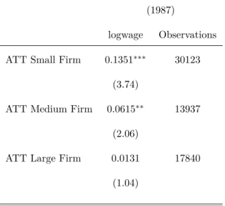
Table 5: Differences in the ATT by Size (1987)
logwage Observations ATT Small Firm 0.1351∗∗∗
30123 (3.74)
ATT Medium Firm 0.0615∗∗
13937 (2.06)
ATT Large Firm 0.0131 17840
(1.04)
tstatistics in parentheses
∗p <0.1,∗∗p <0.05,∗∗∗p <0.01
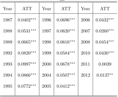
The possible threat to this analysis, as already discussed in the methodology, is that the firms who hire a college graduate do so because they expect positive reasons. Having this threat in mind I repeat the estimations adding one more covariate - the sales of the company in the previous year. If indeed, firms that hire were already in a positive cycle and hired because of it, we should be able to see it in a higher level of sales the previous period. Using this variable as a covariate would then match on it too so the treatment effect would disappear. Before estimating, I point out that I was already using wages of the previous period as a covariate which in principle could already eliminate partially this effect, nevertheless, I add sales to make sure that the spillover found is caused by the hiring and not because of rent-sharing.
Again, there are no significant changes in the results, and the treatment effect continues to be around 5%.8
8
Table 6: ATT when Lagged Sales are Added
Year ATT Year ATT Year ATT
1987 0.0402∗∗∗ 1996 0.0696∗∗∗ 2006 0.0432∗∗∗
1988 0.0531∗∗∗
1997 0.0620∗∗∗
2007 0.0260∗∗∗
1989 0.0665∗∗∗
1998 0.0616∗∗∗
2008 0.0454∗∗∗
1992 0.0820∗∗∗
1999 0.0584∗∗∗
2010 0.0430∗∗∗
1993 0.0997∗∗∗
2000 0.0678∗∗∗
2011 0.0039 1994 0.0866∗∗∗ 2004 0.0507∗∗∗ 2012 0.0137∗∗
1995 0.0772∗∗∗ 2005 0.0412∗∗∗
t statistics in parentheses
∗p <0.1,∗∗ p <0.05,∗∗∗ p <0.01
VII. Additional Results
In Section III I explained why I chose to look at the entry of the first graduate. Nevertheless, to expand a little bit the focus of this thesis, in this section I procceed to the evaluation of the effects of the entry of a second graduate, or better said, of the second hiring of graduates. For this I am going to look at the firms which had already one graduate, and then hire more, most of them will be hiring the second, but some will hire 2 at once or more, like previously. A thing that must be said is that these results will necessarily be much less accurate as the number of observations falls steadily to 401,083. This happens because now the firms that can be subject to the treatment are firms with 1 graduate instead of 0 and this is a much smaller number.
the ones that follow because the knowledge that the second graduate may bring in to the company may be in some way equal to the one brought by the first.
Table 7: ATT for the Entrance of the Second Graduate
(1987) (1988) (1989) (1992) (1993) (1994) (1995) logwage logwage logwage logwage logwage logwage logwage ATT -0.0099 0.0365 0.0202 0.0250 0.0374 0.0449∗∗
0.0248 (-0.37) (1.36) (0.76) (1.09) (1.48) (2.29) (1.16)
N 4386 4753 4854 6063 6317 6690 7596
Off Support 35 94 160 61 19 148 123
tstatistics in parentheses
∗p <0.1,∗∗p <0.05,∗∗∗p <0.01
(1996) (1997) (1998) (1999) (2000) (2004) (2005) logwage logwage logwage logwage logwage logwage logwage ATT 0.0202 0.0248 0.0149 0.0259 0.0223∗ 0.0184 -0.0108
(1.04) (1.39) (0.90) (1.59) (1.76) (1.34) (-0.77)
N 8011 8981 10140 11074 14040 18951 21108
Off Support 51 169 20 268 177 50 142
tstatistics in parentheses
(2006) (2007) (2008) (2009) (2010) (2011) (2012) logwage logwage logwage logwage logwage logwage logwage ATT -0.0139 0.0090 0.0100 0.0063 0.0156 0.0022 -0.0183
(-1.20) (0.76) (0.87) (0.52) (1.28) (0.19) (-1.47)
N 24467 26387 27266 26693 23777 23055 21690
Off Support 514 417 155 363 269 253 223
tstatistics in parentheses
∗p <0.05,∗∗ p <0.01,∗∗∗ p <0.001
VIII. Conclusion
I have used the method of propensity score matching to evaluate how the entry of the first graduate in a firm benefits the productivity of his co-workers. I find evidence that there is a positive spillover of this hiring, which is around 5%. This value while meaningful is smaller than the 11% increase by average year of education that can be found in the literature of education spillovers in Great Britain and maybe in the same order of magnitude of the one found by Martins for Portugal, 3% per average year of education. Nevertheless, it is hard to make these comparisons and the results of this thesis should not be extended to average education. The evidence found shows that the hiring of the first graduate is an important step in the development of a firm and it also tells us that human capital externalities exist at a college level of education. This means that there are reasons for education to be subsidized, because in choosing his level of investment in human capital an individual would not take these positive external effects into account.
Different specifications were tried to test the robustness of the results and no significant changes are found. Furthermore, this thesis presents evidence that smaller firms benefit more from the entry of the first graduate. To be more specific, firms with 5 or less employees face a spillover of approximately 11.6% If we believe that the mechanism by which these spillovers occur is share of knowledge this is no surprise because in smaller firms, there are more interactions between all workers and the college graduate, where they can learn from him.
Further research on education spillovers is left open after this result. To begin with, the database from Quadros de Pessoal, having information on the job title of each worker, allows one to evaluate if the entry of a college graduate to the position of manager, for example, has a higher impact on the productivity of his peers. This would be a research which would be interesting to see not only because of its results, but also because it could provide further robustness to the results of this thesis. Similarly research on which sectors have higher spillover would be of interest and if indeed these sectors are the ones where more interaction between workers is expected. Despite the fact that this thesis points in the direction of share of knowledge as the mechanism for spillovers, this is not really established therefore research on what the mechanism for the spillovers is, would also bring new information to the Labor Economics literature.
Another interesting addition to this thesis would be a different kind of analysis with instrumental variables instead of matching. In fact, I have tried to perform this analysis as an additional robustness test using, firstly, the data of number of graduates by municipality from the Censos and then from Quadros de Pessoal itself, nevertheless, I have faced a problem of weak instrumental variable. Maybe a better instrumental variable can be found which can shed even more light in the trustworthiness of the results presented here. Hopefully, the findings of this thesis will stimulate in other researchers the motivation to carry this research.
References
[1] Acemoglu, Daron (1996), “A Microfoundation for Social Increasing Returns in Human Capital Accumulation”, The Quarterly Journal of Economics, Vol. 111, No. 3 (Aug., 1996), pp. 779-804 [2] Acemoglu, Daron and Joshua Angrist (2000), "How large are Human Capital Externalities?
Ev-idence from Compulsory Schooling Laws", NBER Macroeconomics Annual, Vol. 15 (2000), pp. 9-59
[3] Angrist, Joshua and Alan Krueger (1991), "Does Compulsory School Attendance Affect School-ing and EarnSchool-ings?", The Quarterly Journal of Economics, November 1991, Vol. 106 Issue 4, pp.979-1014
[5] Bartel, Ann P. and Frank R. Lichtenberg (1987), "The Comparative Advantage of Educated Workers in Implementing New Technology", The Review of Economics and Statistics, Vol. 69, No. 1 (Feb., 1987), pp. 1-11
[6] Barth, Erling (2002) “Spillover Effects of Education on Co-Worker Productivity. Evidence from the Wage Structure”, paper presented at the European Society of Population Economics Annual Conference, Bilbao
[7] Battu, H., C. R. Belfield and P. J. Sloane (2003), "Human Capital Spillovers within the Workplace: Evidence for Great Britain", Oxford Bulletin of Economics and Statistics, 65: pp. 575–594. doi: 10.1111/j.1468-0084.2003.00062.x
[8] Blundell, Richard and Mónica Costa Dias (2002), "Alternative Approaches to Evaluation in Em-pirical Microeconomics"
[9] Bound, John David A. Jaeger and Regina M. Baker (1995), "Problems with Instrumental Variables Estimation When the Correlation Between the Instruments and the Endogenous Explanatory Variable is Weak", Journal of the American Statistical Association, June 1995, Vol. 90, No. 430, Applications and Case Studies
[10] Branchflower, David G., Andrew J. Oswald and Peter Sanfey (1996), "Wages, Profits, and Rent-Sharing", The Quarterly Journal of Economics, Vol. 111, No. 1 (Feb., 1996), pp. 227-251
[11] Bryson, A., R. Dorsett, and S. Purdon (2002), "The Use of Propensity Score Matching in the Evaluation of Labour Market Policies", Working Paper No. 4, Department for Work and Pensions [12] Caliendo, Marco and Sabine Kopeinig (2005), "Some Practical Guidance for the Implementation
of Propensity Score Matching", IZA DP No. 1588
[13] Card, David (1995), "Using Geographic Variation in College Proximity to Estimate the Return to Schooling". In L.N. Christofides, E.K. Grant, and R. Swidinsky, editors, Aspects of Labor Market Behaviour: Essays in Honour of John Vanderkamp . Toronto: University of Toronto Press, 1995 [14] Ciccone, Antonio and Giovanni Peri (2006), "Identifying Human-Capital Externalities: Theory
with Applications", Review of Economic Studies (2006) 73, pp. 381–412
[16] Drake, Christiana (1993), "Effects of Misspecification of the Propensity Score on Estimators of Treatment Effect", Biometrics, Vol. 49, No. 4 (Dec., 1993), pp. 1231-1236
[17] Falk, Armin and Andrea Ichino (2006), "Clean Evidence on Peer Effects; Journal of Labor Eco-nomics", Vol. 24, No. 1 (January 2006), pp. 39-57
[18] Gille, Veronique (2011), "Education spillovers in farm productivity: empirical evidence in rural India"
[19] Griliches, Zvi (1969), "Capital-Skill Complementarity", The Review of Economics and Statistics, Vol. 51, No. 4 (Nov., 1969), pp. 465-468
[20] Guryan, Jonathan, Kory Kroft, and Matthew J. Notowidigdo. 2009. "Peer Effects in the Work-place: Evidence from Random Groupings in Professional Golf Tournaments." American Economic Journal: Applied Economics, 1(4): pp. 34-68
[21] Heckman, James, Hidehiko Ichimura and Petra Todd (1997), "Matching as an Econometric Evalu-ation Estimator: Evidence from Evaluating a Job Training Programme", The Review of Economic Studies, Vol. 64, No. 4, Special Issue: Evaluation of Training and Other Social Programmes (Oct., 1997), pp. 605-654
[22] Heckman, James, Hidehiko Ichimura and Petra Todd (1998), "Matching As An Econometric Evaluation Estimator", Review of Economic Studies (1998) 65, pp. 261-294
[23] Iranzo, Susana and Giovanni Peri (2009), "Schooling Externalities, Technology, and Productivity: Theory and Evidence from U.S. States", The Review of Economics and Statistics, May 2009, Vol. 91, No. 2, pp. 420-431
[24] Jovanovic, Boyan and Rafael Rob (1989), "The Growth and Diffusion of Knowledge", The Review of Economic Studies, Vol. 56, No. 4 (Oct., 1989), pp. 569-582
[25] Kandel, Eugene and Edward Lazear (1992), "Peer Pressure and Partnerships, The Journal of Political Economy", Vol. 100, No. 4 (Aug., 1992), pp. 801-817
[26] Lee, Myoung-Jae, "Micro-Econometrics for Policy, Program and Treatment Effects"
[28] Lucas, Robert (1988) “On the Mechanics of Economic Development”, Journal of Monetary Eco-nomics, 22, pp. 3-42
[29] Manski, Charles F. (1993), "Identification of Endogenous Social Effects: The Reflection Problem", The Review of Economic Studies, Vol. 60, No. 3. (Jul., 1993), pp. 531-542
[30] Marshall, Alfred (1890), “Principles of Economics”
[31] Martins, Pedro (2004), "Firm-level social returns to education", IZA DP No. 1382
[32] Mas, Alexander and Enrico Moretti (2009), "Peers at Work", American Economic Review 2009, 99:1, pp. 112–145
[33] Mellow, Wesley (1982), "Employer Size and Wages", The Review of Economics and Statistics", Vol. 64, No. 3 (Aug., 1982), pp. 495-501
[34] Metcalfe, Renuka and Peter J. Sloane (2007), "Human Capital Spillovers and Economic Perfor-mance in the Workplace in 2004: Some British Evidence", IZA DP No. 2774
[35] Mincer, Jacob (1974) “Schooling, Experience and Earnings”, National Bureau of Economic Re-search, New York.
[36] Moretti, Enrico (2004), "Estimating the social return to higher education: evidence from longitu-dinal and repeated cross-sectional data", Journal of Econometrics 121 (2004), pp. 175 – 212
[37] Moretti, Enrico (2004), "Workers’ Education, Spillovers, and Productivity: Evidence from Plant-Level Production Functions", The American Economic Review, June 2004, Vol. 94 No. 3
[38] Rauch, James (1993), "Productivity Gains From Geographic Concentration of Human Capital: Evidence From the Cities", Journal of Urban Economics, 1993, vol. 34, issue 3, pp. 380-400
[39] Rosenbaum, Paul R. (1992), "Detecting Bias with Confidence in Observational Studies", Biometrika, Vol. 79, No. 2 (Jun., 1992), pp. 367-374
[40] Rosenbaum, Paul R. and Donald B. Rubin (1983), "The Central Role of the Propensity Score in Observational Studies for Causal Effects", Biometrika, Vol. 70, No. 1. (Apr., 1983), pp. 41-55
[42] Silva, João Cerejeira da (2003), "Local Human Capital Externalities or Sorting? Evidence From a Displaced Workers Sample"
[43] Spence, Michael (1973), "Job Market Signaling", The Quarterly Journal of Economics , Vol. 87, No. 3. (Aug., 1973), pp. 355-374
[44] Venniker, Richard, "Social returns to education: a survey of recent literature on human capital externalities"
Appendix
(1987)
Variable Treated Control Bias t P-value Variances Ratio
logwage0 4.9483 4.944 0.9 0.28 0.783 1.05
tenure 84.107 83.71 0.7 0.19 0.851 1.13
hab_1 0.05956 0.06021 -0.4 -0.13 0.893 0.90
hab_2 0.47866 0.47464 1.2 0.35 0.728 0.99
hab_3 0.1503 0.14972 0.3 0.08 0.934 1.10
hab_4 0.12358 0.1249 -0.7 -0.19 0.850 1.03
hab_5 0.16529 0.1684 -1.5 -0.37 0.712 1.01
age_25 0.2217 0.2246 -1.2 -0.38 0.706 1.11
age_26_45 0.55951 0.56013 -0.2 -0.07 0.941 1.18
log_size 2.8735 2.8708 0.2 0.06 0.952 0.99
male 0.59176 0.58823 1.0 0.29 0.770 1.04
(1988)
logwage0 4.9648 4.962 0.6 0.18 0.854 1.25
tenure 79.809 79.642 0.3 0.08 0.933 1.14
hab_1 0.0597 0.06008 -0.3 -0.08 0.934 0.94
hab_2 0.47993 0.4728 2.2 0.68 0.497 0.96
hab_3 0.15598 0.15927 -1.5 -0.51 0.612 0.97
hab_4 0.12456 0.1253 -0.4 -0.12 0.908 1.05
hab_5 0.16584 0.16768 -0.9 -0.24 0.811 0.89
age_25 0.22592 0.22808 -0.9 -0.31 0.757 1.08
age_26_45 0.54881 0.5479 0.3 0.12 0.904 1.16
log_size 2.9436 2.9348 0.8 0.22 0.827 0.95
male 0.62566 0.62154 1.2 0.38 0.702 1.00
(1989)
logwage0 5.0948 5.051 -0.3 -0.08 0.934 1.06
tenure 77.645 78.273 -1.0 -0.31 0.753 1.10
hab_1 0.05229 0.05265 -0.3 -0.08 0.933 0.89
hab_2 0.4459 0.44445 0.4 0.14 0.892 0.98
hab_3 0.15599 0.1573 -0.6 -0.20 0.841 1.07
hab_4 0.14027 0.14215 -1.0 -0.27 0.785 1.04
hab_5 0.1876 0.1871 0.2 0.06 0.952 0.97
age_25 0.23131 0.23117 0.1 0.02 0.985 1.16
age_26_45 0.55131 0.54936 0.7 0.25 0.801 1.12
log_size 2.8668 2.865 0.2 0.05 0.963 0.97
male 0.60018 0.59894 0.4 0.11 0.910 1.04
(1992)
logwage0 5.129 5.1263 0.6 0.19 0.852 1.08
tenure 70.882 70.673 0.3 0.11 0.909 1.19
hab_1 0.03693 0.03647 0.4 0.13 0.896 1.00
hab_2 0.40501 0.40022 1.4 0.48 0.633 0.97
hab_3 0.18434 0.18363 0.3 0.10 0.918 1.08
hab_4 0.15694 0.16217 -2.4 -0.75 0.453 1.00
hab_5 0.19832 0.19856 -0.1 -0.03 0.977 1.00
age_25 0.23482 0.2361 -0.5 -0.19 0.852 1.14
age_26_45 0.54808 0.54709 0.4 0.13 0.895 1.22
log_size 2.7379 2.729 0.8 0.24 0.810 1.00
(1993)
Variable Treated Control Bias t P-value Variances Ratio
logwage0 5.1571 5.16 -0.6 -0.19 0.851 0.99
tenure 71.706 72.62 -1.5 -0.49 0.622 1.21
hab_1 0.03111 0.03144 -0.3 -0.11 0.916 0.93
hab_2 0.40091 0.40197 -0.3 -0.10 0.917 1.01
hab_3 0.17907 0.17835 0.3 0.11 0.916 1.08
hab_4 0.15357 0.15516 -0.7 -0.24 0.813 1.00
hab_5 0.21313 0.21119 0.8 0.23 0.822 0.99
age_25 0.22493 0.22569 -0.3 -0.11 0.910 1.10
age_26_45 0.55723 0.55279 1.6 0.61 0.542 1.11
log_size 2.6943 2.693 0.1 0.03 0.973 0.95
male 0.56885 0.56524 1.0 0.35 0.730 1.01
(1994)
logwage0 5.1895 5.1866 0.5 0.21 0.830 1.04
tenure 79.428 79.455 -0.0 -0.02 0.986 1.24
hab_1 0.03291 0.03302 -0.1 -0.04 0.968 0.88
hab_2 0.36098 0.35853 0.7 0.30 0.761 0.98
hab_3 0.18414 0.18527 -0.4 -0.20 0.844 1.05
hab_4 0.18445 0.18989 -2.3 -0.89 0.372 0.97
hab_5 0.20886 0.20472 1.7 0.59 0.553 0.96
age_25 0.2184 0.21891 -0.2 -0.09 0.928 1.22
age_26_45 0.56507 0.56447 0.2 0.10 0.922 1.21
log_size 2.6145 2.6159 -0.1 -0.04 0.965 0.93
male 0.53253 0.52813 1.2 0.50 0.618 1.09
(1995)
logwage0 5.1892 5.1889 0.1 0.02 0.984 1.10
tenure 73.416 74.022 -1.0 -0.38 0.705 1.20
hab_1 0.02541 0.02529 0.1 0.05 0.961 1.04
hab_2 0.3464 0.33977 1.9 0.76 0.448 1.03
hab_3 0.18477 0.18431 0.2 0.08 0.940 1.02
hab_4 0.1867 0.19034 -1.5 -0.56 0.577 1.01
hab_5 0.22625 0.2306 -1.7 -0.54 0.588 0.97
age_25 0.229 0.22923 -0.1 -0.04 0.972 1.14
age_26_45 0.55974 0.55848 0.4 0.19 0.852 1.17
log_size 2.6066 2.5913 1.4 0.47 0.642 0.94
male 0.55925 0.55423 1.4 0.52 0.602 1.09
(1996)
logwage0 5.1842 5.1862 -0.4 -0.15 0.882 1.05
tenure 74.296 40.918 -1.0 -0.39 0.694 1.25
hab_1 0.02313 0.02373 -0.6 -0.24 0.807 1.08
hab_2 0.32525 0.32087 1.3 0.53 0.598 1.00
hab_3 0.19754 0.19823 -0.2 -0.11 0.912 1.00
hab_4 0.18097 0.18319 -0.9 -0.36 0.720 0.98
hab_5 0.2404 0.24111 -0.3 -0.09 0.929 0.96
age_25 0.22211 0.22148 0.2 0.10 0.917 1.23
age_26_45 0.57157 0.57006 0.5 0.23 0.817 1.18
log_size 2.6041 2.5958 0.8 0.26 0.794 0.91
(1997)
Variable Treated Control Bias t P-value Variances Ratio
logwage0 5.1883 5.1945 -1.2 -0.47 0.637 1.04
tenure 71.013 71.509 -0.8 -0.34 0.735 1.19
hab_1 0.0211 0.02166 -0.6 -0.26 0.795 0.92
hab_2 0.32279 0.32065 0.6 0.27 0.788 1.02
hab_3 0.18338 0.17979 1.3 0.62 0.534 1.06
hab_4 0.18112 0.18159 -0.2 -0.08 0.937 0.98
hab_5 0.25645 0.26061 -1.5 -0.53 0.595 0.96
age_25 0.22091 0.21898 0.8 0.34 0.736 1.15
age_26_45 0.56301 0.56261 0.1 0.06 0.949 1.16
log_size 2.5309 2.5122 1.8 0.63 0.529 0.89
male 0.53567 0.53505 0.2 0.07 0.945 1.05
(1998)
logwage0 5.1954 5.1964 -0.2 -0.09 0.931 1.07
tenure 71.366 71.803 -0.7 -0.33 0.743 1.19
hab_1 0.01823 0.01872 -0.5 -0.27 0.786 0.96
hab_2 0.31485 0.31049 1.3 0.61 0.545 1.02
hab_3 0.18697 0.18453 0.9 0.46 0.647 1.05
hab_4 0.18673 0.18777 -0.4 -0.19 0.850 1.03
hab_5 0.25134 0.25705 -2.1 -0.81 0.415 0.94
age_25 0.21602 0.21379 0.9 0.43 0.669 1.18
age_26_45 0.56547 0.56715 -0.6 -0.29 0.770 1.20
log_size 2.4699 2.4554 1.4 0.56 0.577 0.88
male 0.53885 0.53504 1.0 0.47 0.641 1.05
(1999)
logwage0 5.2144 5.2202 -1.2 -0.46 0.649 1.04
tenure 70.1 70.868 -1.3 -0.52 0.604 1.17
hab_1 0.01855 0.01828 0.3 0.13 0.893 1.05
hab_2 0.29534 0.19211 0.9 0.41 0.678 1.03
hab_3 0.18751 0.18401 1.2 0.59 0.552 1.06
hab_4 0.18824 0.19145 -1.3 -0.52 0.603 1.04
hab_5 0.26622 0.27046 -1.5 -0.53 0.597 0.99
age_25 0.2021 0.20148 0.2 0.11 0.913 1.21
age_26_45 0.57938 0.57719 0.7 0.34 0.736 1.20
log_size 2.4799 2.4633 1.7 0.58 0.565 0.87
male 0.53478 0.53122 1.0 0.39 0.698 1.07
(2000)
logwage0 5.2009 5.2022 -0.3 -0.15 0.883 1.10
tenure 69.916 70.178 -0.4 -0.26 0.797 1.14
hab_1 0.01891 0.01941 -0.5 -0.34 0.734 0.89
hab_2 0.31333 0.30811 1.5 0.94 0.347 1.03
hab_3 0.18939 0.18678 0.9 0.64 0.524 1.05
hab_4 0.19273 0.19429 -0.6 -0.36 0.718 1.06
hab_5 0.25845 0.26408 -2.0 -1.01 0.312 0.96
age_25 0.19162 0.19083 0.3 0.21 0.836 1.24
age_26_45 0.57562 0.57477 0.3 0.19 0.850 1.18
log_size 2.4008 2.3852 1.6 0.83 0.408 0.84
(2004)
Variable Treated Control Bias t P-value Variances Ratio
logwage0 5.1676 5.1731 -1.1 -0.58 0.561 1.06
tenure 65.578 65.953 -0.6 -0.36 0.718 1.26
hab_1 0.01769 0.01707 0.6 0.39 0.696 1.09
hab_2 0.24607 0.24206 1.2 0.72 0.475 1.05
hab_3 0.2007 0.19675 1.3 0.83 0.408 1.10
hab_4 0.23457 0.23677 -0.7 -0.42 0.677 1.08
hab_5 0.26841 0.27426 -1.9 -0.95 0.348 0.99
age_25 0.16481 0.1638 0.4 0.25 0.802 1.27
age_26_45 0.59546 0.59543 0.0 0.01 0.995 1.20
log_size 2.128 2.1121 1.8 0.85 0.396 0.79
male 0.55705 0.55765 -0.2 -0.09 0.931 1.13
(2005)
logwage0 5.1625 5.1642 -0.3 -0.19 0.848 1.11
tenure 62.588 62.335 0.4 0.27 0.784 1.30
hab_1 0.01746 0.01786 -0.4 -0.25 0.801 0.99
hab_2 0.24635 0.24362 0.8 0.51 0.611 1.08
hab_3 0.2171 0.21302 1.3 0.87 0.385 1.12
hab_4 0.22988 0.22936 0.2 0.11 0.915 1.06
hab_5 0.25669 0.2644 -2.5 -1.32 0.187 1.00
age_25 0.16323 0.16217 0.5 0.29 0.775 1.21
age_26_45 0.60143 0.60155 -0.0 -0.02 0.981 1.18
log_size 2.1154 2.1011 1.6 0.81 0.415 0.77
male 0.60492 0.60693 -0.5 -0.30 0.761 1.20
(2006)
logwage0 5.135 5.1414 -1.3 -0.85 0.394 1.13
tenure 66.449 66.461 -0.0 -0.02 0.988 1.26
hab_1 0.01647 0.01587 0.6 0.49 0.621 0.99
hab_2 0.24799 0.24311 1.4 1.05 0.294 1.09
hab_3 0.20119 0.19562 1.8 1.47 0.141 1.15
hab_4 0.23833 0.23844 -0.0 -0.03 0.979 1.10
hab_5 0.26674 0.27687 -3.2 -2.05 0.041 1.03
age_25 0.14634 0.1457 0.3 0.22 0.829 1.28
age_26_45 0.60336 0.60351 -0.0 -0.04 0.971 1.22
log_size 2.0779 2.0588 2.1 1.34 0.179 0.83
male 0.59874 0.5989 -0.0 -0.03 0.978 1.22
(2007)
logwage0 5.1518 5.157 -1.0 -0.67 0.505 1.10
tenure 67.258 67.095 0.3 0.19 0.848 1.13
hab_1 0.01584 0.01484 1.1 0.81 0.420 1.06
hab_2 0.25542 0.25384 0.5 0.33 0.742 1.10
hab_3 0.2156 0.21201 1.2 0.87 0.385 1.12
hab_4 0.23318 0.23093 0.7 0.53 0.594 1.09
hab_5 0.24934 0.25701 -2.4 -1.51 0.131 1.03
age_25 0.13653 0.13517 0.6 0.46 0.649 1.26
age_26_45 0.60134 0.60398 -0.8 -0.63 0.528 1.21
log_size 2.064 2.0492 1.7 1.00 0.316 0.80
(2008)
Variable Treated Control Bias t P-value Variances Ratio
logwage0 5.1941 5.1943 -0.0 -0.03 0.978 1.03
tenure 66.171 66.208 -0.1 -0.04 0.969 1.17
hab_1 0.01272 0.01234 0.4 0.32 0.748 1.06
hab_2 0.20351 0.19912 1.4 0.92 0.357 1.11
hab_3 0.19229 0.18754 1.6 1.11 0.267 1.10
hab_4 0.26445 0.26309 0.4 0.28 0.783 1.10
hab_5 0.29092 0.30139 -3.2 -1.78 0.075 1.00
age_25 0.1351 0.13445 0.3 0.20 0.845 1.27
age_26_45 0.59996 0.60111 -0.4 -0.25 0.806 1.21
log_size 2.0536 2.0372 1.8 0.98 0.326 0.80
male 0.57889 0.57474 1.1 0.65 0.516 1.17
(2009)
logwage0 5.207 5.2082 -0.2 -0.13 0.893 1.12
tenure 69.133 69.397 -0.4 -0.24 0.807 1.30
hab_1 0.01182 0.01206 -0.3 -0.18 0.859 1.09
hab_2 0.18461 0.18125 1.1 0.68 0.498 1.13
hab_3 0.19021 0.18835 0.6 0.39 0.695 1.16
hab_4 0.26131 0.26165 -0.1 -0.06 0.949 1.09
hab_5 0.31169 0.31432 -0.8 -0.40 0.686 1.02
age_25 0.12855 0.12651 1.0 0.57 0.571 1.24
age_26_45 0.59175 0.5927 -0.3 -0.18 0.856 1.19
log_size 1.9548 1.9454 1.1 0.53 0.595 0.74
male 0.56072 0.5581 0.7 0.38 0.706 1.17
(2010)
logwage0 5.246 5.2476 -0.3 -0.17 0.861 1.03
tenure 75.141 74.861 0.4 0.24 0.811 1.23
hab_1 0.01001 0.00992 0.1 0.08 0.940 1.07
hab_2 0.17795 0.17534 0.9 0.52 0.600 1.11
hab_3 0.18188 0.17974 0.7 0.46 0.647 1.13
hab_4 0.27758 0.2761 0.5 0.26 0.793 1.12
hab_5 0.31715 0.32277 -1.7 -0.84 0.402 1.05
age_25 0.11461 0.11367 0.5 0.27 0.791 1.30
age_26_45 0.58856 0.58944 -0.3 -0.16 0.871 1.22
log_size 1.9352 1.9224 1.5 0.71 0.480 0.79
male 0.56255 0.55968 0.7 0.40 0.687 1.21
(2011)
logwage0 5.2589 5.2611 -0.4 -0.22 0.829 1.05
tenure 69.588 69.217 0.6 0.30 0.762 1.29
hab_1 0.00742 0.00686 0.7 0.48 0.634 1.56
hab_2 0.15688 0.15338 1.2 0.67 0.505 1.13
hab_3 0.18419 0.18083 1.1 0.63 0.531 1.13
hab_4 0.29193 0.29044 0.4 0.23 0.818 1.09
hab_5 0.32292 0.33143 -2.4 -1.12 0.262 1.01
age_25 0.11623 0.11479 0.7 0.35 0.726 1.24
age_26_45 0.60675 0.60683 -0.0 -0.01 0.991 1.20
log_size 1.9106 1.8928 2.1 0.91 0.365 0.75
(2012)
Variable Treated Control Bias t P-value Variances Ratio
logwage0 5.3316 5.3324 -0.2 -0.10 0.923 1.13
tenure 76.3 75.997 0.4 0.23 0.818 1.21
hab_1 0.00775 0.0079 -0.2 -0.12 0.903 1.01
hab_2 0.15635 0.1533 1.0 0.57 0.569 1.10
hab_3 0.18372 0.1796 1.3 0.75 0.451 1.15
hab_4 0.30025 0.2968 1.0 0.52 0.606 1.11
hab_5 0.31768 0.32854 -3.1 -1.41 0.159 1.00
age_25 0.11102 0.11185 -0.4 -0.20 0.841 1.21
age_26_45 0.58859 0.58791 0.2 0.10 0.916 1.19
log_size 1.8841 1.8691 1.7 0.76 0.448 0.79
male 0.5403 0.53975 0.1 0.07 0.946 1.12
(1987) (1988)
logwage Observations logwage Observations ATT Small Firm 0.1352∗∗∗
30123 0.1272∗∗∗
31962
(3.74) (3.72)
ATT Medium Firm 0.0615∗∗
13937 0.1098∗∗∗
15196
(2.06) (3.73)
ATT Large Firm 0.0131 17840 0.0133 18857
(1.04) (1.08)
(1989) (1992)
logwage Observations logwage Observations ATT Small Firm 0.1554∗∗∗ 35332 0.1410∗∗∗ 57964
(4.96) (6.52)
ATT Medium Firm 0.1050∗∗∗
16856 0.0667∗∗
11746
(4.18) (2.50)
ATT Large Firm 0.0274∗∗
20333 0.0152 15076
(2.28) (1.13)
tstatistics in parentheses
(1993) (1994)
logwage Observations logwage Observations ATT Small Firm 0.1769∗∗∗ 62443 0.1450∗∗∗ 63740
(7.84) (8.01)
ATT Medium Firm 0.1114∗∗∗
12182 0.0869∗∗∗
11959
(4.45) (3.71)
ATT Large Firm 0.0215 14707 0.0144 14256
(1.60) (1.22)
(1995) (1996)
logwage Observations logwage Observations ATT Small Firm 0.1542∗∗∗
79090 0.1272∗∗∗
81659
(8.07) (6.81)
ATT Medium Firm 0.0453∗∗ 12934 0.0857∗∗∗ 12673
(2.02) (4.03)
ATT Large Firm 0.0078 14547 0.0099 13836
(0.65) (0.79)
(1997) (1998)
logwage Observations logwage Observations ATT Small Firm 0.1192∗∗∗
89026 0.1144∗∗∗
96770
(7.38) (7.56)
ATT Medium Firm 0.0498∗∗∗
13697 0.0311∗
14319
(2.62) (1.75)
ATT Large Firm 0.0136 14289 0.0064 14394
(1.24) (0.60)
tstatistics in parentheses
(1999) (2000)
logwage Observations logwage Observations ATT Small Firm 0.0921∗∗∗ 103824 0.1051∗∗∗ 112473
(5.71) (9.50)
ATT Medium Firm 0.0337 14982 0.0373∗∗∗
16491
(1.60) (2.80)
ATT Large Firm 0.0268∗∗
14264 0.0170∗
15385
(2.28) (1.92)
(2004) (2005)
logwage Observations logwage Observations ATT Small Firm 0.0738∗∗∗
148119 0.0692∗∗∗
156575
(7.00) (7.00)
ATT Medium Firm 0.0239∗ 17124 0.0182 17008
(1.75) (1.38)
ATT Large Firm 0.0086 13266 0.0140 13152
(0.76) (1.26)
(2006) (2007)
logwage Observations logwage Observations ATT Small Firm 0.0715∗∗∗
168254 0.0524∗∗∗
167985
(9.13) (6.27)
ATT Medium Firm 0.0084 17141 0.0072 16568
(0.78) (0.64)
ATT Large Firm 0.0027 13608 -0.0048 12958
(0.29) (-0.44)
tstatistics in parentheses
(2008) (2009)
logwage Observations logwage Observations ATT Small Firm 0.0590∗∗∗ 168238 0.0578∗∗∗ 168062
(6.36) (6.22)
ATT Medium Firm 0.0352∗∗∗
15946 0.0447∗
14849
(2.79) (3.26)
ATT Large Firm 0.0093 12021 0.0222∗
10552
(0.83) (1.68)
(2010) (2011)
logwage Observations logwage Observations ATT Small Firm 0.0574∗∗∗
142345 -0.0048 139973
(6.08) (-0.55)
ATT Medium Firm 0.0299∗∗ 12764 0.0015 11665
(2.26) (0.11)
ATT Large Firm 0.0027 8770 -0.0005 7919
(0.23) (-0.04)
(2012)
logwage Observations ATT Small Firm 0.0154∗ 133205
(1.76)
ATT Medium Firm 0.0053 10154 (0.36)
ATT Large Firm 0.0086 6880
(0.59)
tstatistics in parentheses