pag. 1
Flat-Tax and Minimum Income
Experiment in an OLG model of Italy
Giacomo Scalabrin
Dissertation written under the supervision of
João
Brogueira de Sousa
Dissertation submitted in partial fulfilment of requirements for the MSc in
Macroeconomic Policy, at the Universidade Católica Portuguesa, 13/09/2019.
pag. 2
ABSTRACT:
In the light of the recent political events in Italy this paper aims to quantitatively analyze the impact of a Flat-Tax and minimum income based fiscal reform for different cohort ages in an Overlapping Generation (OLG) model with permanent labour productivity across agents and a stochastic labour income component. Two Computational Experiments are conducted: the former is a Flat-Tax only for the personal labour income, the latter involves the same marginal rate for personal labour and capital income. It results that to finance a minimum income measure in support of every citizen below the absolute poverty threshold, it is required a marginal rate of respectively 20% and 23%. The amount granted would be equal to the difference of the absolute poverty threshold (€780 in Italy) and the total income of the targeted citizen. The results of this study seem to reflect the forecasts of overall growth in the aggregate output and consumption of the economy: a deeper analysis show that actually the labour supplied and aggregate welfare decrease while the inequality considerably increases.
SOMARIO:
À luz dos recentes eventos políticos em Itália, este artigo visa analisar quantitativamente o impacto de uma reforma fiscal baseada na renda fixa e no imposto mínimo para diferentes idades de coorte num modelo de Overlapping Generation (OLG) com produtividade permanente do trabalho entre agentes e um componente estocástico do rendimento trabalho. Duas Experiências Computacionais são conduzidas: a primeira é um imposto fixo somente para a renda de trabalho pessoal, a segunda envolve a mesma taxa marginal para trabalho pessoal e capital. Resulta que, para financiar uma medida de rendimento mínimo, de forma a apoiar todos os cidadãos abaixo da limiar de pobreza absoluta, é necessária uma taxa marginal de respectivamente 20% e 23%. A quantia admitida seria igual à diferença do limiar de pobreza absoluta (€780 na Itália) e a renda total do cidadão visado. O resultado deste estudo parece refletir as previsões de crescimento da produção e consumo agregados à economia: uma análise mais profunda mostra que, na verdade, a mão-de-obra fornecida e o bem-estar agregado diminuem enquanto a desigualdade aumenta consideravelmente.
ACKNOWLEDGEMENTS:
I would like to thank my advisor João Brogueira de Sousa, who have been following me along the all dissertation period and suggested the direction more times during my path. Thanks you for appreciating my ideas and allowing me to learn more about macroeconomics equilibrium models and to grow as an economist. A special thank to my parents, who are the most valuable persons in the world to me. Thanks you for allowing me to study, travel, to follow my dreams and finally to find happiness in my life. Thanks you for the sacrifices and your patience. Finally, a special thanks to all the friends that sustained me during all my permanence in Catolica. Without you it wouldn’t have been the same experience.
pag. 3
Summary
1 Introduction ... 5
1.1 The 2018 Italian fiscal-benefits system ... 8
1.1.1 Pro-poor measures evolution in Italy ... 9
2 OLG models: literature review ... 9
2.1 The baseline OLG model structure ... 10
2.1.1 The Diamond model ... 10
2.2 literature evolution of OLG models ... 10
2.2.1 Generations and cohort size ... 10
2.2.2 Individual heterogeneity ... 11
2.2.3 Demographic changes introduced by immigration ... 11
2.2.4 OLG Models with Government and Social Security ... 11
3 Methodology: overview of the model ... 11
3.1 Demographics ... 11
3.2 Endowments, preferences and agents’ heterogeneity. ... 12
3.3 Firms ... 13
3.4 Government policy ... 13
3.5 The structure of the market ... 14
3.6 The competitive equilibrium ... 14
3.6.1 Households ... 15
3.6.2 Firms ... 15
3.6.3 Social security system ... 15
3.6.4 Transfers ... 15
3.6.5 Government ... 15
3.6.6 Market clearing ... 15
3.6.7 Law of motion ... 16
3.7 Computing the equilibrium: The Python program ... 16
4 Calibration of the benchmark economy ... 17
4.1 Demographics ... 17
4.2 Preferences ... 18
4.3 The labour productivity process ... 18
4.4 Technology ... 20
4.5 Government ... 20
4.5.1 Consumption tax (IVA) ... 20
pag. 4
4.5.3 Separate Capital Income tax ... 21
4.5.4 Personal Labour Income tax (IRPEF) ... 21
4.5.5 The “Reddito d’Inclusione” - REI ... 22
4.5.6 Individual tax function specification T[.] ... 22
4.6 The benchmark economy ... 23
5 Computational experiment: a Flat-Tax and minimum income reform ... 24
5.1 Result of the first experiment: a Flat-Tax on the personal labour income ... 25
5.2 Result of the second experiment: a Flat Tax on the personal labour and capital income ... 27
6 Discussing the results ... 29
6.1 First experiment: 20% Flat-Tax on the individual labour income... 29
6.2 Second experiment: 23% Flat-Tax on individual labour and capital income ... 34
6.3 Comparing the Computational Experiments ... 38
7 Conclusion ... 38 Bibliography ... 40 APPENDIX 1: ... 42 APPENDIX 2: ... 46 APPENDIX 3 ... 47 APPENDIX 4 ... 48
pag. 5
1 Introduction
Italy’s coming through a tough period during the last years. 2018 in particular has seen concerning breackdowns in the peninsula’s economy. Above the many issues, two seems to be the major problems: on the one hand the estimated 190 billion euros of fiscal evasion and a tax gap of 23,28% that place the country in the worst position among the EU members. On the other an alarming unemployment rate, especially for early age citizens; with the 39,5% of young workers unemployed, in December 2018 Italy registered in fact the second highest rate in Europe.
The GDP growth forecasts for 2019 are not optimistic: they range from the +0,6% of the Monetary Fund to the more problematic -0,2% estimated few weeks ago by OCSE. According to these previsions, and the aggravating circumstance that the Quantitative Easing just stopped, the Italian ground seems not to leave any margin for a sustainable debt, that would indeed require an economic growth rate higher than the interest paid on the debt itself.
2018 have been a troubled year also for the Italian political scene. Never in the history of the peninsula’s republic it happened to wait so much for a definitive election: five rounds of consultations, two exploratory terms for the presidents of the House and Senate and two pre-mandates. The Giuseppe Conte government (M5s-Lega) finally have established obtaining the majority of the consensus largely due to the promise of two reforms: “Flat-Tax 15%” for the personal labour income, to replace the current progressive IRPEF tax, and “Reddito di Cittadinanza”, a pro-poor minimum income measure, and unemployment benefit, that would be granted from the mid of 2019 to citizens receiving less than the estimated absolute poverty threshold: only together these two measures should, according to the major M5s-Lega economists’ opinion, stimulate and boost the economy. However the positions on the matter diverge within the country and a great debate has risen during the last year especially about the affordability of these two expensive measures, estimated to cost around 80 billion euros: to grant an minimum amount to poor citizens together with the promise of a consistent cut in the taxes seems hardly implementable in the common sense without lowering the public expenditure, increasing the consumption tax or the public debt, but renewed M5s-Lega economists such as Claudio Borghi, Alberto Bagnai and Michele Geraci still claim that it is sustainable and that the Italian economy will benefit from the reform.
In Italy firms are not able to find skilled young workers, and young people cannot find job: this incompatibility represents one of the major concerns for the economic recovery as demand and supply don’t meet each other. A minimum income, besides being a pro-poor measure that an advanced economy should implement for an ethic fairness, would allow for an improvement in the efficiency of the labour force, by the moment that young people can so find an occupation that suites better their personal skills without the concern of being unemployed. On the other hand, even if this can improve
pag. 6 the efficiency of the allocation of the human capital, Italy also required a reform to increase the labour demand, that is to create new jobs: a constant marginal rate of 15% attract new investments, and with them new jobs opportunities. Regarding the costs of these measures, according to the abovementioned economists, it would be partially compensated by the increase of the aggregate consumption level. That is, through the Keynesian multiplier the GDP of the country should grow at a bigger share than the expenditure for these measures.
Moreover, a Flat-Tax 15% discourage tax evasion. In most of the countries that have adopted similar fiscal schemes the historical evidence (look for instance Keen (2006) and Hall (2013)) as taught that a simpler tax system enhances the tax compliance: if citizens, instead of living in a complex and abstruse fiscal system, are more aware on how much taxes they have to pay to the government and they perceive them as a fair amount, than they should be more inclined to the “fiscal loyalty”. But again, after one year of political mandate and public discussion, it is nowadays still not clear where the government would find the money for this reform, and the persistent lack of quantitative studies on the matter does not help to consolidate an objective position about it. As economist, it is in my interest to further investigate on the possible outcomes of such a reform and to provide some results that quantify the impact that a fiscal system based on a Flat-Tax and a minimum income would have on Italian citizens in different ages.
In a good number of studies focusing on optimal taxation it results that a Flat-Tax based fiscal system brings gains in term of labour supply, consumption and capital accumulation, compared to a progressive one. Conesa and Krueger (2006) compute the optimal progressivity of the labour income tax for US in an Overlapping Generation model, accounting for household’s heterogeneity. It is so quantitatively characterized the optimal income tax system in an economic environment where insurance, equity and efficiency effects are present simultaneously. The main quantitative result found is that the optimal income tax structure is well approximated by a flat income tax and a fixed deduction; under such a reform, most of the agents obtain welfare gains and according to their outcomes the middle-income households are the ones that would suffer the most (they would face a higher income tax bill), whereas both high-income and low-income households would benefit. Similar results reflect Ventura (1999)’s findings and are supported by Mankiw, Weinzierl and Yagan
(2009). Aaberge, Colombino and Storm (2004) conduct an analysis of the welfare effects on married
couples of replacing the Italian progressive tax system by three alternative hypothetical reforms: a Flat-Tax, a negative income tax, and a work fare scheme. The results suggest that there are margins for improvement upon the current system for both the efficiency and the equality criterion. According to their outcomes the estimated benefits of the reform would come from a good response in the labour
pag. 7 supply of poor and middle-class households, whereas the wealthier citizens appear to be much less responsive to changes in the tax rates. Scutella (2004) studied the implications of the introduction of a basic income and Flat-Tax system in Australia in a General Equilibrium and microeconomic model. To provide a basic income levels coinciding with current benefits rates results to be costly, with a marginal rate required to ensure revenue neutrality that turns out unsustainable. Such a system, while more equitable and social welfare enhancing than the one in use at the time, was found to have likely adverse labour supply responses confounding the cost of the system. Shubert (2018) quantifies the economic effects of a Flat-Tax and minimum income reform proposal for Germany. The effects are negligible, even negative for what regard the level of employment and GDP within the country: these results cast doubts on whether such a fundamental reform would have positive welfare effects. About tax evasion and avoidance, it is possible to find studies in support of a progressive fiscal system. For instance, Gamannossi and D. Rablen (2017) basing on the work of Alm and McCallin
(1990) describe avoidance as a risky asset owing to the possibility of effective anti-avoidance
measures by the tax authority: they consider then the implications for optimal auditing of tax avoidance. By analyzing the audit function under progressive, proportional and regressive tax systems they find that less enforcement is required under a flat tax than under a progressive one in eliminating evasion and avoidance, for every level of income. This outcome confirms Chander and Wilde (1998) findings, according to which a regressive tax results to be the optimal hypothetical fiscal system in term of tax evasion and avoidance.
This paper aims to analyze and quantify the outcome for households in different ages, of a Flat-Tax and a minimum income measure reforming the progressive fiscal system in Italy. This is done employing an Overlapping Generations Model with permanent labour productivity across agents and an idiosyncratic stochastic component, calibrated to reflect the empirical evidence found in microeconometrics studies based on Italians’ data. Two Computational Experiments are conducted: - The first is a Flat-Tax reforming the current progressive IRPEF tax on the individual labour income. The marginal rate is derived so that the government finances a minimum income targeting all agents under the absolute poverty threshold (quantile 0.084 of the income distribution according to ISTAT), keeping fixed the public expenditure. The amount granted to each individual under that limit is computed as the difference between the poverty threshold and his total earnings.
- The second experiment is analogous to the first one. The difference consists in setting the same flat marginal rate for both the individual labour and capital income.
pag. 8 The paper is structured as follow: in the following paragraph it will be exposed the 2018 Italian fiscal system. Chapter 2 provides a brief review on OLG models. In Chapter 3 it is reported the model employed for this study. Chapter 4 and 5 describe respectively the process of calibration of the benchmark economy and the Computational Experiments. To follow Chapter 6, in which the results are discussed, and finally Chapter 7 concludes the paper.
1.1 The 2018 Italian fiscal-benefits system
The Italian fical system is national with little differences among regions and municipalities due to some local autonomy and mainly affecting the complex system of local property taxes. The individual labour income tax (IRPEF) is progressive and incomes deriving from capital gains and return on capital are mainly subject to a separate taxation. The main source through which the government raises funds for public expenditure are:
- Personal labour Income Tax – IRPEF: a progressive tax on income structured in five brackets. The taxable base is the total income (sum of working income, buildings and lands income, quotes from dividends, dividends gains) and family dimension and composition for eventual deductions and allowances.
- Separate Taxation on Capital Income: capital income, even though already partially included in the IRPEF base, is mainly subject to a separate taxation.
- Municipality Property Taxes – IMU and TASI: buildings and lands, like capital income, are subject to a separate taxation. IMU and TASI weight on buildings or lands’ owners or to individuals who enjoy real rights on these estates.
- Corporate Tax – IRES: It is a proportional tax applied to all corporations, cooperatives, mutual insurance, public and private entities other than the special companies. The premise for the Corporate Tax is the ownership of an income belonging to one of the following categories: real estate, capital, employed and self-employed work, corporation.
- Regional Tax on Business – IRAP: a special regional tax on productive activities located in the area of regional competence. Therefore, it is applied to companies and individuals subject to IRES, companies subject to personal income tax (partnerships and sole proprietorships), banks, insurance companies and self-employed workers. The rate change according to the business sector.
Italy, like most of the modern developed countries, is characterized by a fragmented benefits system, made of a multitude of instruments. According to the tradition, these social measures can be categorized in Social Insurance (family and social allowances, benefits related to the end of the working activity, to the temporary suspension of the working activity, to the reduction in working
pag. 9 ability) and Social Assistance (family support, Pro-poor allowances, Benefits related to the reduction in working ability). Thresholds for means-tested benefits and contributions are yearly updated by the National Statistical Office.
Finally, the Social Contributions that employees, employers and self-employed individuals pay on earned income that are managed by the National Institute of Social Security (INPS), a private entity that regulates the pension system within the country. An exhaustive description of the measures composing the 2018 Italian fiscal and benefits system can be found in Appendix 1.
1.1.1 Pro-poor measures evolution in Italy
During the past decades Italy, as many advanced modern countries, have started to develop instruments pro-poor oriented to fight the wealth inequalities across the country. The design of a national measure of minimum guaranteed income has started in 1997 with a first proposal formulated by the ‘Commissione Onofri’ appointed by the Centre-Left government in power at that time. The proposal has been tested in a sample of local areas before being stopped when a Centre-Right came to power two years later: the competence on support policies was so transferred to the regions, which since then effectively became responsible for the design of pro-poor policies.
A more recent national minimum income scheme, the ‘Reddito di Inclusione- REI’ was proposed in 2017 by the ‘Goveno Gentiloni’ and have been implemented in 2017: this instrument is meant to address the share of the population living in absolute poverty and aims to fill the gap between the resources available in the families and the minimum level of income required to fulfill their fundamental needs. Unfortunately, even though it was designed to be universal, the available funds have been sufficient to accomplish only partially the desired goal, and overall the REI barely impacted the fraction of the population that was meant to sustain.
2 OLG models: literature review
Macroeconomic models provide an efficient tool for analyzing the impact of fiscal and policies in more or less complex representations of real economies. A wide number of models have been created to date and offer different combination of features such as agents’ heterogeneity, multiple sectors, overlapping generations, adequate treatment of uncertainty and expectations. The exponential technological and theoretical progress in general or partial equilibrium models has reached insights that would not have been possible with simpler models and their limits. These tools have become the framework to use to conduct a quantitative analysis of a fiscal policy and so to be able to carry on a comprehensive evaluation of the dangers and potentials of a reform. In this literature review it is provided a fast background on OLG models and on the diversity and complexity that may be introduced.
pag. 10 2.1 The baseline OLG model structure
Overlapping Generation (OLG) models analyze the general equilibrium properties and growth dynamics of economies inhabited by finitely lived population in different cohorts ages: incorporating demographic transition, they have the potential to increase the predictive power compared to models with infinitely lived agents. They became popular mainly thanks to the seminal works carried on by
Diamond (1965) and Auerbach and Kotlikoff (1987).
The core process in an OLG model follows the choices of a representative household regarding variables such as education, savings, labour supply and according to a utility function that regulate his/her preferences: this allow to project the wealth distribution for agents in different cohorts ages over time.
2.1.1 The Diamond model
The most basic, two-period OLG model consists in a close economy with only firms and households (no government) and exogeneous labour. In this model agents supply labour and receive an income in return, that will spend on consumption or savings to invest in capital, since they own the firms. The whole amount invested in the first period is consumed in the second one. If 𝑁𝑡 denote the size of young generation of agents and 𝑁𝑡−1 the old cohorts, and assuming a constant rate 𝑛, 𝑠𝑜 𝑁𝑡 = (1 + 𝑛)𝑁𝑡−1. The young generation supplies one unit of labour (exogeneous variable) in exchange of a
fixed income 𝑤𝑡 and chooses how to allocate it between consumption and savings. In the next period the same generation becomes old and retire, so live with the investments made previously.
2.2 literature evolution of OLG models 2.2.1 Generations and cohort size
Extending the same concept of the basic Diamond OLG model, the literature has evolved considering more than just two period. For instance, a four-period OLG model have been elaborated by Buyse et
al (2012) with three working generations, heterogeneous in labour choice, leisure and skills and one
retired. Magnani and Mercenier (2009) study the variation of choices for retired individuals in different cohort ages employing an eight-period setup with five working generations and three retired. The recent literature has extended the analysis to include up to 100 generations of age groups: these models allow to generate predictions of consumption and saving decisions that at times closely resemble the target economy (for instance Muto et al. 2012; Beetsma and Bucciol 2009; Cerný et al.
2006). Additional studies can be mentioned, as the one of Kudrna et al. (2014) in which individuals
aged 0 to 20 can rely on the public system for education and healthcare costs, reducing the amount granted for pensions to the retiree.
pag. 11 2.2.2 Individual heterogeneity
Including additional intra-generations heterogeneity allows to produce a more realistic variety of consumption and savings paths. One of the sources of heterogeneity that has been employed in most of these studies comes by assuming that agents are born in different ability levels: ability becomes then a productivity factor that impact individuals’ earnings. Fougère and Mérette (1999) propose a spill-over model in which the aggregate savings depend on the post-secondary education of the agents in the economy. A similar heterogeneity source can be found in Magnani and Mercenier (2009) or either in Buyse et al. (2012).
2.2.3 Demographic changes introduced by immigration
OLG models provides an excellent tool in the field of study that analyses the migration of agents from one market to another. Many traditional models fail to capture this complex aspect of one economy: the major issue is that the savings, labour choices and consumption patterns can diverge consistently between citizens and immigrants. Fougère et al. (2004), to mention one, analyze the immigration phenomenon in Canada employing a six-region OLG model.
2.2.4 OLG Models with Government and Social Security
To conclude this fast overview on OLG models, they provide a useful framework to analyze the effect of government policies and reforms. Bucciol et al. (2014) study different policies in an OLG model with heterogeneous agents modelling the joint labour supply choices between man and women in a couple. The analysis is conducted for three European countries: France, Italy and Sweden. They show that the model is capable of matching relevant aggregate statistics of the three countries and provide examples of policy experiments that can be simulate, analyzing the outcomes on both inequality and individual welfare. Conesa, Kitao and Krueger (2007) compute the optimal progressive capital and labor income tax in an OLG model with stochastic income shocks, where households are heterogeneous in ability level. They find that the optimal capital income tax rate approximates a Flat-Tax of 23% with a fix deduction corresponding to about $6,000.
The model employed in this study follows the guidelines of the Conesa, Kitao and Krueger (2007) one, with adjustments made to better reflect the 2018 Italian economy and fiscal system. A full description follows in Chapter 3.
3 Methodology: overview of the model
3.1 Demographics
The economy examined for this study is populated by 𝐽 overlapping generations. Every year a continuum of new agents is born, and the overall population grows at a fix rate 𝑛. Each household faces a probability of dying in every period, which is dependent on the age. In specific, the probability
pag. 12 of being alive in period 𝑗 + 1 conditional being alive in period 𝑗, is 𝜓𝑗 = 𝑝𝑟𝑜𝑏(𝑎𝑙𝑖𝑣𝑒 𝑎𝑡 𝑗 + 1|𝑎𝑙𝑖𝑣𝑒 𝑎𝑡 𝑗). Households can live up to a maximum age 𝐽, so that 𝜓𝐽 = 0. The fraction of the agents who dies in every period before reaching age 𝐽 leaves accidental bequests, denoted by 𝑇𝑟𝑡, that are
redistributed in a lump-sum manner across the population. At age 𝑗𝑟 households retire and receive a pension 𝑆𝑆𝑡 that is financed by a flat income tax 𝜏𝑠𝑠,𝑡. The Social Security taxes base is labour income 𝑦.
3.2 Endowments, preferences and agents’ heterogeneity.
Each household starts his life without assets (besides the eventual bequests distributed) and can supply up to one unit of productive time every period. They can either spend their time working in a competitive market or consuming leisure. Their consumption-leisure preferences {𝑐𝑗, (1 − 𝑙𝑗)}𝑗=1𝐽 are represented by the following standard time-separable utility function:
𝐸 (∑ 𝛽𝑗−1
𝐽
𝑗=1
(𝑐𝑗ϒ(1 − 𝑙𝑗)1−ϒ)1−𝜎
1 − 𝜎 ) (1)
where 𝑐𝑗 and 𝑙𝑗 are respectively the level of consumption and labour in period 𝑗. The parameter ϒ
measures how important is consumption relative to leisure, and 𝜎 controls the degree of risk aversion. Finally, 𝛽 is the time discount factor.
In this model three sources of heterogeneity are considered to better represent the Italian households’ labour productivity:
- An age-specific labor productivity component ԑ𝑗: households of different ages have a different
age productivity ԑ𝑗. After the retirement age 𝑗𝑟, by assumption the agents’ productivity is set equal to zero, that is ԑ𝑗 = 0.
- Households differ in abilities 𝛼𝑖 : they are born and live as one of M possible ability types
𝑖 𝜖 𝐼. It is not possible for them to switch from an ability type to another during their lifetime. The probability of being born with ability 𝛼𝑖 is denoted by 𝑝𝑖 > 0. The ability type 𝛼𝑖 in addition to age-specific productivity component ԑ𝑗, determine agents’ average deterministic
labor productivity, the permanent component of this labour productivity process.
- Agents of the same ability type and with the same age differ in an idiosyncratic uncertainty with respect to their labor productivity, that represent the last component of agents’ heterogeneity in this model. The stochastic process describing labor productivity status is the same across all the agents and follows a finite-state Markov chain with stationary transitions, described by:
pag. 13
𝑄𝑡(ƞ, 𝐸) = 𝑃𝑟𝑜𝑏(ƞ𝑡+1 𝜖 𝐸|ƞ𝑡= ƞ) = 𝑄(ƞ, 𝐸) (2)
Here ƞ𝑡 𝜖 𝐸 denotes a stochastic realization of the labor productivity in time 𝑡. Households start their life at the same average productivity level ƞ = ∑ ƞ𝛱(ƞ)ƞ where ƞ 𝜖 𝐸 and 𝛱(ƞ) is the probability of ƞ under the stationary distribution. The stochastic process manifests different realizations for labour productivity, and so generates cross-sectional productivity, income and wealth distribution that become more dispersed as the cohorts grow. The agents maximize their expected utility in a lifetime prospective. These expectations are taken with respect to the stochastic processes that leads to the idiosyncratic labor productivity.
Every agent is characterized in a given time by the measures (𝑎𝑡, ƞ𝑡, 𝑖, 𝑗), where 𝑎𝑡 are the asset holdings (of one period, risk-free bonds), ƞ𝑡 is stochastic labor productivity status at date t, 𝑖 is the ability type and 𝑗 is the age. An agent of type (𝑎𝑡, ƞ𝑡, 𝑖, 𝑗) choose to work 𝑙𝑗 hours and then earn
pre-tax labor income ԑ𝑗𝛼𝑖ƞ𝑡𝑙𝑗𝑤𝑡, that depend on the wage per efficiency unit of labor 𝑤𝑡, the age specific productivity component ԑ𝑗, the ability type 𝛼𝑖 and the state ƞ𝑡. φ𝑡(𝑎𝑡, ƞ𝑡, 𝑖, 𝑗) denote the probability
measure of agents of type (𝑎𝑡, ƞ𝑡, 𝑖, 𝑗). 3.3 Firms
The technology describing the firms’ production process is represented by a Cobb–Douglas production function with constant return to scale. As standard with a perfect competition market it is assumed the existence of a representative firm operating this technology. The resource constraint is given by the following function:
𝐶𝑡+ 𝐾𝑡+1− (1 − 𝛿)𝐾𝑡+ 𝐺𝑡 ⩽ 𝐴𝑡𝐾𝑡𝛼𝑁𝑡1−𝛼 (3) Here 𝐶𝑡 , 𝐾𝑡 and 𝑁𝑡 represent respectively the aggregate consumption, capital stock and labour supply in time 𝑡. The term 𝐴𝑡 = (1 + 𝑔)𝑡−1𝐴1 captures the technological progress.
The calibration of 𝐴, as in Conesa, Kitao and Krueger (2007), is normalized to 1: in accordance with similar studies on fiscal policies evaluation this paper abstract from technological progress. In this way it allows to represent households in the economy with a labour supply elasticity that is consistent with the microeconometric evidence.
3.4 Government policy
The government levies taxes to finance public spending and runs a balanced budget social security system represented in the model by the transfers 𝑆𝑆𝑡. The tax rate 𝜏𝑠𝑠,𝑡 is set to assure that the budget balance of the system time by time. The pulic consumption {𝐺𝑡}𝑡=1∞ is given exogenously and has three fiscal instruments to be financed: the government levies a proportional tax 𝜏𝑐,𝑡 on consumption
pag. 14 expenditures, it tax capital income of households 𝑟𝑡(𝑎𝑡+ 𝑇𝑟𝑡) according to a constant tax rate 𝜏𝐾,𝑡,
and finally levies a personal income tax on each individual’s labour income. The income of an agent before the social security tax is defined as 𝑦𝑝𝑡= 𝑤𝑡ԑ𝑗𝛼𝑖ƞ𝑙𝑡 (4) and depend on the wage per efficiency unit of labor 𝑤𝑡. A part of the social contribution, in specific one third in Italy, is paid by the employer: the model takes this into account. This part is represented by 𝑒𝑠𝑠𝑡 = 0.33𝜏𝑠𝑠,𝑡𝑤𝑡ԑ𝑗𝛼𝑖ƞ𝑙𝑡 (5).The income base for the personal labour income tax of a household is so defined as:
𝑦𝑡 = {𝑦𝑝𝑡− 𝑒𝑠𝑠𝑡 𝑖𝑓 𝑗 < 𝑗𝑟 0 𝑖𝑓 𝑗 ≥ 𝑗𝑟
(6)
The individual tax function is 𝑇[. ], and 𝑇[𝑦] is the total tax liability on a labour income equal to 𝑦. 3.5 The structure of the market
In this economy agents cannot insure against stochastic labor income shocks by trading insurance contracts. They can however trade one period risk-free bonds to insure themselves against the risk of a decrease of their labor productivity in the future. This is limited, however, by impossibility of agents to sell bonds short. Basically, a stringent borrowing constraint is imposed upon all agents to prevents them from dying in debt, in presence of the positive conditional probability of death.
3.6 The competitive equilibrium
In this paragraph it is defined the competitive and stationary equilibrium in this economy (see Definition 1 and 2 below), following the same baseline of Conesa, Kitao and Krueger (2007), with little adjustments mainly regarding the .For each agent, the state variables describing his status are personal asset holdings 𝑎, labor productivity ƞ, ability type 𝑖 and age 𝑗. The aggregate picture of the overall economy in a given time 𝑡 is described by the agents’ measure φ𝑡 over asset positions, labor productivity status, ability and age.
Let 𝑎 𝜖 𝑹+, ƞ 𝜖 𝐸 = {ƞ1, ƞ2, … , ƞ𝑛}, 𝑖 𝜖 𝐼 = {1,2, … , 𝑀}, j 𝜖 𝐽 = {1,2, … , 𝐽}, and 𝑺 = 𝑹+∗ 𝐸 ∗ 𝐼 ∗ 𝐽.
Let 𝑩(𝑹+) be the Borel σ-algebra of 𝑹+ and 𝑷(𝐸), 𝑷(𝐼), 𝑷(𝐽) the power sets of 𝐸, 𝐼 and 𝐽. Let M
be the set of al finite measure over the measurable space (𝑺, 𝑩(𝑹+) ∗ 𝑷(𝐸) ∗ 𝑷(𝐼) ∗ 𝑷(𝐽)).
Definition 1: Given a sequence of social security replacement rates {𝑏𝑡}𝑡=1∞ , consumption tax rates
{𝜏𝑐,𝑡}𝑡=1∞ and government expenditure {𝐺𝑡}𝑡=1∞ and initial conditions 𝐾1 and φ1, a competitive equilibrium is a sequence of functions for the household, {𝑣𝑡, 𝑐𝑡, 𝑎′
𝑡, 𝑙𝑡∶ 𝑺 → 𝑹+}𝑡=1∞ of production
plans for the firm, {𝑁𝒕, 𝐾𝒕}𝑡=1∞ , government income tax functions {𝑇
𝑡 ∶ 𝑹+ → 𝑹+}𝑡=1∞ , social security
taxes { 𝜏𝑠𝑠,𝑡}𝑡=1∞ and benefits {𝑆𝑆𝑡}𝑡=1∞ , prices {𝑤𝒕, 𝑟𝒕}𝑡=1∞ , transfers {𝑇𝑟𝒕}𝑡=1∞ , and measures {φ𝒕}𝑡=1∞ ,
pag. 15 3.6.1 Households
Given prices, policies, transfers and initial conditions, for each time, the agent choose the value 𝑣𝑡 that maximizes the Bellman equation (where 𝑐𝑡, 𝑎′
𝑡 and 𝑙𝑡 are his policy functions):
𝑣𝑡(𝑎, ƞ, 𝑖, 𝑗) = 𝑚𝑎𝑥 𝑐,𝑎′,𝑙 (𝑢(𝑐, 1 − 𝑙) + 𝛽𝜓𝑗∫ 𝑣𝑡+1(𝑎 ′, ƞ′, 𝑖, 𝑗 + 1)𝑄(ƞ, 𝑑ƞ′)) (7) subject to: (1 + 𝜏𝑐,𝑡 )𝑐 + 𝑎′ = (1 − 0.66𝜏𝑠𝑠,𝑡) 𝑤𝑡 1+0.33𝜏𝑠𝑠,𝑡ԑ𝑗𝛼𝑖ƞ𝑙𝑡+ (1 + 𝑟𝑡(1 − 𝜏𝐾,𝑡)) (𝑎 + 𝑇𝑟𝑡) − 𝑇𝑡[𝑦𝑡] if 𝑗 < 𝑗𝑟 (8) (1 + 𝜏𝑐,𝑡 )𝑐 + 𝑎′ = 𝑆𝑆𝑡+ (1 + 𝑟𝑡(1 − 𝜏𝐾,𝑡)) (𝑎 + 𝑇𝑟𝑡) − 𝑇𝑡[𝑆𝑆𝑡] if 𝑗 ≥ 𝑗𝑟, (9) 𝑎′ ≥ 0, 𝑐 ≥ 0, 0 ≤ 𝑙 ≤ 1 (10) 3.6.2 Firms
In equilibrium, prices 𝑤𝒕 and 𝑟𝒕 satisfy:
𝑟𝑡 = 𝛼𝐴𝑡( 𝑁𝑡 𝐾𝑡 ) 1−𝛼 − 𝛿 (11) 𝑤𝑡= (1 − 𝛼)𝐴𝑡( 𝐾𝑡 𝑁𝑡 ) 𝛼 (12)
3.6.3 Social security system the pensions policies satisfy:
𝜏𝑠𝑠,𝑡= ∫(𝑤𝑡ԑ𝑗𝛼𝑖ƞ𝑙𝑡)φ𝑡(d𝑎 ∗ dƞ ∗ d𝑖 ∗ 𝑑𝑗) = 𝑆𝑆𝑡∫ φ𝑡(d𝑎 ∗ dƞ ∗ d𝑖 ∗ { 𝑗𝑟 , … , 𝐽})
(13)
3.6.4 Transfers
The accidental bequests are defined as are given by:
𝑇𝑟𝑡+1∫ φ𝑡+1(d𝑎 ∗ dƞ ∗ d𝑖 ∗ 𝑑𝑗) = ∫(1 − 𝜓𝑗) 𝑎′𝑡(𝑎, ƞ, 𝑖, 𝑗)φ𝒕(d𝑎 ∗ dƞ ∗ d𝑖 ∗ d𝑗)
(14)
3.6.5 Government
Government budget balances as follows:
𝐺𝑡= ∫ 𝜏𝐾,𝑡𝑟𝑡(𝑎 + 𝑇𝑟𝑡)φ𝒕(d𝑎 ∗ dƞ ∗ d𝑖 ∗ d𝑗) + ∫ 𝑇𝑡[𝑦𝑡]φ𝒕(d𝑎 ∗ dƞ ∗ d𝑖 ∗ d𝑗)
+ 𝜏𝑐,𝑡∫ 𝑐𝑡(𝑎, ƞ, 𝑖, 𝑗)φ𝒕(d𝑎 ∗ dƞ ∗ d𝑖 ∗ d𝑗) (15)
3.6.6 Market clearing
𝐾𝑡 = ∫ 𝑎φ𝒕(d𝑎 ∗ dƞ ∗ d𝑖 ∗ d𝑗) (16)
pag. 16 ∫ 𝑐𝑡(𝑎, ƞ, 𝑖, 𝑗)φ𝒕(d𝑎 ∗ dƞ ∗ d𝑖 ∗ d𝑗) + 𝑎′𝑡(𝑎, ƞ, 𝑖, 𝑗)φ𝒕(d𝑎 ∗ dƞ ∗ d𝑖 ∗ d𝑗) + 𝐺𝑡 = 𝐾𝑡𝛼(𝐴𝑡𝑁𝑡)1−𝛼+ (1 − 𝛿)𝐾𝑡 (18) 3.6.7 Law of motion φ𝒕+𝟏 = 𝐻𝑡(φ𝑡) (19)
where the function 𝐻𝑡∶ 𝑴 → 𝑴 can be explicitly written as:
a) for all ꝭ such that 1 𝜖 ꝭ:
φ𝒕+𝟏(A ∗ E ∗ Ꝭ ∗ ꝭ) = ∫ 𝑃𝑡((𝑎, ƞ, 𝑖, 𝑗); A ∗ E ∗ Ꝭ ∗ ꝭ)φ𝒕(d𝑎 ∗ dƞ ∗ d𝑖 ∗ d𝑗) (20) where 𝑃𝑡((𝑎, ƞ, 𝑖, 𝑗); A ∗ E ∗ Ꝭ ∗ ꝭ) = {𝑄(𝑒, 𝐸)𝜓𝐽 if 𝑎 ′ 𝑡(𝑎, ƞ, 𝑖, 𝑗) 𝜖 𝐴, 𝑖 𝜖 Ꝭ, 𝑗 + 1 𝜖 ꝭ 0 else (21) b) φ𝒕+𝟏(A ∗ E ∗ Ꝭ ∗ {1}) = (1 + 𝑛)𝑡{∑ 𝑖 𝜖 Ꝭ𝑝𝑖 if 0 𝜖 𝐴, ƞ 𝜖 𝐸 0 else (22)
Definition 2: a stationary equilibrium is a competitive equilibrium in which 𝑏𝑡= 𝑏1, 𝜏𝑐,𝑡 = 𝜏𝑐,1, 𝐺𝑡= (1 + 𝑛)𝑡−1𝐺
1, 𝑎′𝑡(. ) = 𝑎′1(. ), 𝑐𝑡(. ) = 𝑐1(. ), 𝑙𝑡(. ) = 𝑙1(. ), 𝑁𝑡= (1 + 𝑛)𝑡−1𝑁1,
𝐾𝑡 = (1 + 𝑛)𝑡−1𝐾
1, 𝑇𝑡 = 𝑇1, 𝜏𝑠𝑠,𝑡 = 𝜏𝑠𝑠,1, 𝑆𝑆𝑡= 𝑆𝑆1, 𝑟𝑡 = 𝑟1, 𝑤𝑡 = 𝑤1, 𝑇𝑟𝑡 = 𝑇𝑟1, for all 𝑡 ≥ 1 and
for 𝐴 𝜖 𝑹+. That is, per capita variables and functions as well as prices and policies are constant, and
aggregate variables grow at the constant growth rate of the population n. 3.7 Computing the equilibrium: The Python program
This paragraph explains briefly how the Python program coded for this analysis works.
Initally are defined the choices for the last generation, who face no possibility of surviving in the next period: the investment (asset choice) is zero because it is not possible anymore to derive any utility in the future. The labour choice is also zero by the moment they retire at age 65. The consumption and value functions are then computed for agents in every asset level. The consumption coincides with the Social Security and the asset level, net of taxes (on income and on consumption). The value function for every level of asset is the utility function, with zero labour and the consumption previously computed.
For the younger cohort ages the choices distributions are compiled backward (for every asset level). From the age of 98 to 65 no labour is supplied by agents, so the only choice involved is the one on consumption and investment. This choice is derived with respect to the Euler equation (the derivation is reported in Appendix 2):
pag. 17 𝑀𝑎𝑟𝑈𝑡𝑖𝑙𝑖𝑡𝑦(𝑐, 1 − 0) = 𝛽𝜓𝑗∫ (1 + 𝑟𝑡(1 + 𝜏𝑘,𝑡 )) 𝑀𝑎𝑟𝑈𝑡𝑖𝑙𝑖𝑡𝑦(𝑐′, 1 − 0)𝑄(ƞ, 𝑑ƞ′)
(23)
Lower bound and upper bounds are computed (it is derived the utility for the lowest and for the highest level of asset choice) in case the Euler function does not allow a maximum inside this interval assumed for the asset grid.
Once the optimal consumption level is found for every possible asset level, the computation of Value function is straight forward.
𝑉𝑎𝑙𝑢𝑒(𝑐, 1 − 0) = 𝑈𝑡𝑖𝑙𝑖𝑡𝑦(𝑐, 1 − 0) + 𝛽𝜓𝑗∫ 𝑉𝑎𝑙𝑢𝑒(𝑐′, 1 − 0) 𝑄(ƞ, 𝑑ƞ′)
(24)
With 𝑐 and 𝑐′ at the optimal level.
For agents in working age (from 64 to 25 years), the process is substantially the same: the same outcome is derived for every possible choice of work (66 possible from 0 to 0.99) according to the Euler equation:
𝑀𝑎𝑟𝑈𝑡𝑖𝑙𝑖𝑡𝑦(𝑐, 1 − 𝑙) = 𝛽𝜓𝑗∫ (1 + 𝑟𝑡(1 + 𝜏𝑘,𝑡 )) 𝑀𝑎𝑟𝑈𝑡𝑖𝑙𝑖𝑡𝑦(𝑐′, 1 − 𝑙′)𝑄(ƞ, 𝑑ƞ′)
(25)
The value chosen is the work-consumption couplets that maximize the Value function for each agent.
4 Calibration of the benchmark economy
4.1 Demographics
The agents enter in the economy at the age of 25 (that correspond to age 1 in the model), retire at 67 (age 42 in the model) and die at 100 years old (75 in the model).
The data relative to the Italian population growth is taken from Worldometers Real Time Statistics
database, that carries out estimation for the future of the country. The long-term population growth
parameter 𝑛 is calculated as the average annual rate for the period 1965-2040.
Conesa, Kitao and Krueger (2007) use period life tables to compute survival probabilities 𝜓𝑗, while a proper calibration should rather use cohort life tables to not under-estimate the life length. The survival probabilities employed in the model are estimated in Bucciol et al (2014) with data collected by the Human Mortality Database period life tables from 1979 to 2008. They distinguish the trend from fluctuations estimating the parameters of the Lee and Carter model (1992) with a singular value decomposition:
pag. 18 Figure 1: survival probability distribution over life cycle
ln(1 − 𝜓𝑗,𝑡𝑝 ) = 𝛼𝑗+ 𝜏𝑗χ𝑡+ 𝜖𝑗𝜓 (26)
where 𝛼𝑗 and 𝜏𝑗 are age-varying parameters, χ𝑡 is a time-varying vector and 𝜖𝑗𝜓 is a random disturbance distributed as 𝑁(0, ỡ𝜓2). The derived survival probability is reported in Figure 1: these
results are about 3 years higher than official statistics from the World Health Organization (WHO) and similar organizations based on period life tables.
4.2 Preferences
The coefficient of relative risk aversion 𝜎 it’s fixed over time. It is set at the value of 3, compatibly with the estimates found in the literature (see for instance Bucciol et Al (2014), Ventura (1999) and the references therein).
The discount factor 𝛽 is calibrated so that the equilibrium of the benchmark economy implies a capital-output ratio of as observed in the data. According to Gardiner, Waights and Derbyschire
(2011) the estimated capital-outout ration for the year 1995 is 2.75 and this value is compatible with
the value often adopted in the literature.
According to OECD’s estimates in 2018 Italians citizens worked on average 1782 hours; considering that the daily discretionary time of a person is 16 hours (with 8 hours of sleep), Italians worked around 30,5% of their discretionary time. The share of consumption ϒ is calibrated so that the average time that individuals spend working in the model meet this estimate.
4.3 The labour productivity process
In every period each agent alive in the economy is endowed with one unit of time and can spend it either for working or leisure. The labor productivity of each individual is composed of the ability type
pag. 19 𝛼𝑖, the age-specific labour productivity component ԑ𝑗 and the idiosyncratic stochastic component ƞ. The logarithm of wages of a household is therefore given by:
log(𝑤𝑡) + log(𝛼𝑖) + log(ԑ𝑗) + log(ƞ) (27)
The age-productivity profile {ԑ𝑗}𝑗=1 𝑗𝑟−1 employed for this study is taken by Walewsky (2008). His
estimates for Italy in 2004 display the maximum productivity at the age of 46, corresponding to the value of 1.13, as displayed in Figure 2. The wage productivity level is then normalized to 1 around the age of 25 (age 1 in the model) and is set equal to 0 for retired agents, so older than 67 years (43 in the model).
For the calibration of ability-type dependent fixed effect 𝛼𝑖, as for Conesa, Kitao and Krueger (2007), an agent can be born in one of two possible ability type, with equal probability 𝑝𝑖 = 0.5 and fixed
effects 𝛼1 = 𝑒−𝜎𝛼 and 𝛼
2 = 𝑒𝜎𝛼 , so that the expected value 𝐸(log(𝛼𝑖)) = 0 is zero and the variance
of the ability type 𝑉𝑎𝑟(log(𝛼𝑖)) = 𝜎𝛼2 is fixed.
Regarding the definition of the Markov process for the stochastic component of the log-wages it evolves as a discrete AR(1) process with five states, characterized by a persistence parameter р and variance 𝜎ƞ2.
In conclusion, the parameterization of the labour productivity process can be summarizes in the three parameters 𝜎𝛼2, р, 𝜎
ƞ2 to be calibrated. The choice of these parameters targets statistics quantifying
how cross-sectional labor income volatility evolves over the Italian individual’s life cycle: Aktas
(2017) document the life cycle cross-sectional variance of household labor income distribution
estimated for Italy with data that come from the archives of Italian Social Security Administration (INPS), covering the years from 1985 to 2012. In the model employed for this paper labour supply is
pag. 20 endogenous and responds optimally to the productivity process. Aktas (2017) reports a cross sectional variance of 0.58 at the age of 25, and around 1.36 at 60: the three parameters 𝜎𝛼2, р, 𝜎ƞ2 are chosen
so that the in the calibrated benchmark economy this model displays a cross-sectional variance profile consistent with these outcomes, assuming a linear distribution from the age of 25 to 60. For the purpose of the parameterization the Tauchen method is used to discretize the linear AR(1) process and derive the transition probability matrix and the reward vector.
4.4 Technology
The share of capital income on total income 𝛼 = 0.35 is chosen in accordance to the literature on General Equilibrium and OLG models; a similar choice can be found in Bucciol et al. (2014) and in the references therein.
The depreciation rate of capital 𝛿, following Conesa, Kitao and Krueger (2007), is targeted so that in stationary equilibrium the benchmark economy implies an investment to output ratio consistent with the observed one in Italy. CEIC Data, institution that conduct expansive and accurate data insights into both developed and developing economies, provides annual estimates for the national investment over GDP ratio. the reference indicator for the model is 21%, estimation for the year 2018.
The Total Factor of Productivity 𝐴, following Conesa, Kitao and Krueger (2007) is normalized to 1. 4.5 Government
The government finances public expenditure and raise funds for the minimum income through taxes on consumption, capital and labour income and grant an amount (REI) to individuals under a computed threshold. The taxes levels are chosen to represent the 2018 fiscal and benefits system. 4.5.1 Consumption tax (IVA)
The VAT rate in Italy (IVA) is fixed at 22%, with reductions on some category of goods. It is 4% for primary food such as milk, butter, cheese, vegetables, fruits, cereals, etc. On socio-sanitary and educational services the VAT rate is 5%. Finally, on other food that is not primary is 10%. The average consumption expenditure estimated by ISTAT was € 2564 per family in 2017, the 17,8% of which was for food. Primary food consumption accounted for 7,1% and health and education for 5,4%. The fix consumption tax rate parameter employed in the model, 𝜏𝑐,𝑡, is the weighted average
of the different VAT rates weighted for Italians’ consumption habits. 4.5.2 Social Security program
Regarding the social security system, the 66% of the social contributions are paid by the employee and the remaining 33% by the employer. The tax rate 𝜏𝑠𝑠,𝑡 is set to assure that the budget balance of
pag. 21 4.5.3 Separate Capital Income tax
in Italy capital income is not subject to the IRPEF, but to a separate taxation. For income deriving from dividends, obligations, banking and postal interest income, certificates of deposits, and other sources of capital income with less than 18 months of maturity the tax rate is 26%, while for bonds, and similar with maturity longer than 18 months is 12,50%. Because in the model the agents can only invest in one-year risk free bonds, the tax rate on capital gains is set to 26%.
4.5.4 Personal Labour Income tax (IRPEF)
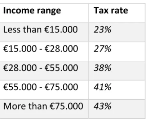
In this paragraph it will be described how the tax function that is levied on the agents’ labour income is composed in this paper to represent the Italian economy. In Italy the tax on labour income is personal and progressive, structured in the five brackets reported in the Table 1. A no tax area is applied for households with income below € 8174 per year, amount that goes close to the estimated absolute poverty threshold of € 780 per month (€9360 a year). According to ISTAT, in 2017 the incidence of absolute poverty in terms of individuals was 8,4%: for this study a poverty threshold matching this estimate is set for the no tax zone.
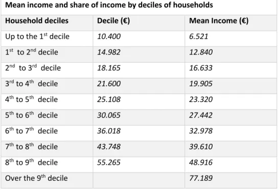
The data provided by the Banca d’Italia in the Survey on Household Income and Wealth in 2014 is reported in Table 2: the brackets’ ranges are set to match these estimates.
Income range Tax rate
Less than €15.000 23% €15.000 - €28.000 27% €28.000 - €55.000 38% €55.000 - €75.000 41% More than €75.000 43%
The quantiles of the income distribution corresponding to the IRPEF brackets are obtained from
Table 2 and Table 3. The amount of 15.000 euros is so set as the second decile. 28.000 is the mean
income above the fifth and sixth decile, 55.000 is the ninth decile and 75.000 is set as the mean income of the last decile. A higher marginal rate is paid only on the part of income exceeding the previous bracket. This does not work for the no-tax area: if an agent earns more than the no tax threshold, must pay taxes on all the labour income.
The Italian fiscal scheme also provides a system of deductions and detractions for the IRPEF; in the model it is included a fix deduction on labour income only for agents earning less than € 55.000 (ninth decile of the income distribution in the model). By the moment that households are represented as
pag. 22 individuals, no family deductions or allowances, or neither any other kind of reduction (eg. for total/partial disability, war servants, etc.) are considered
Mean income and share of income by deciles of households
Household deciles Decile (€) Mean Income (€)
Up to the 1st decile 10.400 6.521 1st to 2nd decile 14.982 12.840 2nd to 3rd decile 18.165 16.633 3rd to 4th decile 21.600 19.905 4th to 5th decile 25.108 23.320 5th to 6th decile 30.065 27.442 6th to 7th decile 36.018 32.978 7th to 8th decile 43.748 39.610 8th to 9th decile 55.265 48.916
Over the 9th decile 77.189
4.5.5 The “Reddito d’Inclusione” - REI
Finally, the benchmark economy calibrated for the 2018 tax-benefits system includes the REI
(Reddito di Inclusione), a pro-poor instrument introduced in 2017 to sustain families with income
under the absolute poverty threshold. The REI is included in the model as a negative income tax (so inside the personal income tax function) and a parameter adjusts the maximum amount that is paid to households and the deduction on the personal labour income tax to clear the market, so that the tax total tax revenue compensates the chosen government expenditure level.
4.5.6 Individual tax function specification T[.]
The individual labour income tax function is specified as follow: 𝑇[𝑦𝑡] = −( 𝑝 ∗ 𝒯 − 𝑦𝑡− 𝑟𝑡(𝑎𝑡+ 𝑇𝑟𝑡)) 𝑖𝑓 𝑦𝑡+ 𝑟𝑡(𝑎𝑡+ 𝑇𝑟𝑡) ≤ 𝑝 ∗ 𝒯 0 𝑖𝑓 𝑦𝑡+ 𝑟𝑡(𝑎𝑡+ 𝑇𝑟𝑡) ≤ 𝒯 0.23 ∗ min (𝑦𝑡− 𝑝 𝑠, 0) 𝑖𝑓 𝒯 ≤ 𝑦𝑡+ 𝑟𝑡(𝑎𝑡+ 𝑇𝑟𝑡) ≤ 𝑏1 0.23 ∗ 𝑏1 + 0.27 ∗ (𝑦𝑡− 𝑏1 − 𝑝 𝑠) 𝑖𝑓 𝑏1 ≤ 𝑦𝑡+ 𝑟𝑡(𝑎𝑡+ 𝑇𝑟𝑡) ≤ 𝑏2 0.23 ∗ 𝑏1 + 0.27 ∗ 𝑏2 + 0.41(𝑦𝑡− 𝑏2 − 𝑝 𝑠) 𝑖𝑓 𝑏2 ≤ 𝑦𝑡+ 𝑟𝑡(𝑎𝑡+ 𝑇𝑟𝑡) ≤ 𝑏3
pag. 23 0.23 ∗ 𝑏1 + 0.27 ∗ 𝑏2 + 0.38 ∗ 𝑏3 + 0.41 ∗ (𝑦𝑡− 𝑏3) 𝑖𝑓 𝑏3 ≤ 𝑦𝑡+ 𝑟𝑡(𝑎𝑡+ 𝑇𝑟𝑡) ≤ 𝑏4
0.23 ∗ 𝑏1 + 0.27 ∗ 𝑏2 + 0.38 ∗ 𝑏3 + 0.41 ∗ 𝑏4 + 0.43(𝑦𝑡− 𝑏4) 𝑖𝑓 𝑦𝑡+ 𝑟𝑡(𝑎𝑡+ 𝑇𝑟𝑡) > 𝑏4
(28)
Where 𝑦𝑡 denotes the individual labour earnings net of social contributions, 𝑟𝑡(𝑎𝑡+ 𝑇𝑟𝑡) the individual capital earnings. 𝒯 is the absolute poverty threshold (computed as quantile 0.084 of the income distribution, according to ISTAT estimates for 2018) and 𝑏1, 𝑏2, 𝑏3 𝑎𝑛𝑑 𝑏4 correspond to the brackets of the progressive labour income tax, set to match the estimates displayed in Table 2 as described in paragraph 4.5.4. Finally 𝑝 and 𝑠 are parameters defining both the minimum income amount granted in the benchmark economy (REI) and the fixed deduction on the individual labour income.
The following observations may be useful for a better understanding of the individual labour tax function 𝑇[𝑦𝑡]:
- 𝑝 ∗ 𝒯 define level of minimum income “REI” granted in the benchmark economy. For instance, if in the stationary equilibrium it is found that 𝑝 equal to 0,5 the minimum income measure will be granted only for citizens with earnings below the half of the absolute poverty threshold within the country, and 𝑝 ∗ 𝒯 is the maximum possible amount granted by the government. This means that an agent earning 200 in an economy where the poverty threshold is 1000, will receive by the government 1000 ∗ 0,5 − 200 = 300. An agent earning 0 receives 500 and to an agent earning 500 nothing will be granted.
- 𝑠 is a parameter meant to proportionate the minimum income amount granted and the fixed deduction on labour income 𝑝
𝑠. This deduction is available for income smaller than €55.000,
so below the ninth decile (Table 2). 4.6 The benchmark economy
To follow a brief commentary on the parametrized benchmark economy. Table 3 lists the relevant variables that are calibrated in the model. The parameterization of the benchmark model has been conducted so these measures result proportionate to the two observed in Italy: the absolute poverty threshold have been estimated by ISTAT to be €780 monthly, the deduction about €8000 for income smaller than €55.000 a year and the maximum amount granted by the government with the REI for a poor individual has been estimated by INPS to be around €200 a month. In the stationary equilibrium the benchmark economy reports a parameter of 0.402, meaning that the 40,2% of the absolute poverty threshold is level of minimum income (REI) granted to an individual before the reform, so about
pag. 24 €310. The fixed deduction 𝑝
𝑠 results 0.0201 (the parameter 𝑠 is set to be 20), value close to the one
of the absolute poverty threshold, as observed in the empirical evidence.
Parametrization
Category Variable Value Target/Source
Demographics population growth 𝑛 0.236% per year Worldomoeters Survival probabilities 𝜓𝑗 distribution Bucciol et Al. (2004)
Age of birth in the model 𝑗1 25 years (1) Birth age (assumed)
Retirement age 𝑗𝑟 67 years (43) Old age retirement
Maximum age 𝐽 100 years (76) Certain death
Preferences Discount factor 𝛽 0.966 K/Y (Gardiner) = 2.75
Risk aversion 𝜎 3 Ventura (1999)
Consumption share ϒ 0.4 Avrg hours worked: 0.305
Labor productivity age-productivity profile ԑ𝑗 distribution Walewsky (2008)
Variance types 𝜎𝛼2 0.2945 Aktas (2017)
Persistence р 0.9394 Aktas (2017)
Variance shock 𝜎ƞ2 0.3841 Aktas (2017)
Technology Capital share 𝛼 0.35 Bucciol et Al. (2004)
Depreciation rate 𝛿 0.077 I/Y (CEIC Data) = 0.21
Scale parameter 𝐴 1 Normalized
Government Consumption tax 𝜏𝑐,𝑡 18,5% ISTAT
Capital income tax 𝜏𝑘,𝑡 26% Short-time cap inc tax
Poverty threshold 𝒯 0.0202 ISTAT (quantile 0.084)
Parameter 𝑝 0.402 Banca d’Italia
Parameter 𝑠 20 MI-deduction proportion
Social security tax 𝜏𝑠𝑠,𝑡 13,3% ISTAT
5 Computational experiment: a Flat-Tax and minimum income reform
The purpose of the study consists in evaluating the effect of a Flat tax and a Minimum Income reform. Once the model is parametrized, it is possible to proceed to the computational experiment. Keeping fixed the level of government spending and the absolute poverty threshold calibrated in the stationary equilibrium of the benchmark economy, a new tax function is defined: this is characterized by a constant marginal rate for the individual income and by a parameter defining the level of minimum income 𝑝 ∗ 𝒯 in favor of the poor agents. Just like for the benchmark economy, a parameter adjusts so that the total tax revenue offsets the fixed government expenditure amount previously calibrated. The goal is to find a marginal rate allowing the government to grant a minimum income level coinciding with the absolute poverty threshold 𝒯, so a marginal rate for which, in the stationary equilibrium, the parameter 𝑝 equals 1; to be clear an agent earning 200 in an economy where the threshold 𝒯 is 1000 will receive 1000 − 200 = 800. Two different experiments are conducted: the first consists in a Flat-Tax reforming only the personal labour income, so keeping the marginal rate
pag. 25 of the capital income unchanged and second involves a unique flat marginal rate for both the individual labour and capital income.
5.1 Result of the first experiment: a Flat-Tax on the personal labour income
The first experiment consists in simulating a Flat-Tax on the personal labour income and in deriving the marginal rate for which the maximum level of Minimum Income granted to the underprivileged individuals in the economy coincides with the poverty threshold. That is, a marginal rate that would allow to solve the absolute poverty issue within the country (so that no agent would earn less than the previously calibrated absolute poverty threshold) keeping fixed the government expenditure level. The personal labour income tax function is so defined as
𝑇[𝑦𝑡] =
−( 𝑝 ∗ 𝒯 − 𝑦𝑡− 𝑟𝑡(𝑎𝑡+ 𝑇𝑟𝑡)) 𝑖𝑓 𝑦𝑡+ 𝑟𝑡(𝑎𝑡+ 𝑇𝑟𝑡) ≤ 𝑝 ∗ 𝒯
𝜏𝑦𝑦𝑡 𝑖𝑓 𝑦𝑡+ 𝑟𝑡(𝑎𝑡+ 𝑇𝑟𝑡) > 𝑝 ∗ 𝒯
(29)
where 𝜏𝑦 is the Flat-Tax’s marginal rate. This rate results to be 20%: the stationary equilibrium reports indeed a parameter of 1,0255 meaning that the level of minimum income granted is the 102,55% of the poverty threshold (look in the Appendix 3).
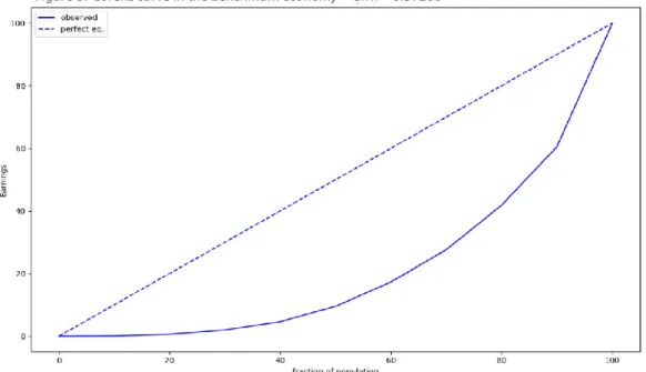
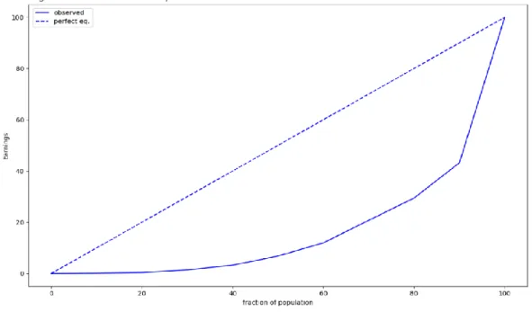
The Gini coefficient is the measure chosen to assess the inequalities within the country and is computed for both the Benchmark economy and the computational experiment: it is a measure of statistical dispersion intended to represent the income distribution of a nation’s residents. It is usually defined mathematically based on the Lorenz curve, which plots the proportion of total income of the
pag. 26 population that is cumulatively earned by the bottom x of the population. A line representing the perfect equality of income is then plotted at 45 degrees. The Gini index is finally computed as the ratio of the area that lies between the perfect equality and the Lorenz curve. Figure 3 and Figure 4 provide a graphical representation of the Lorenz curve for respectively the benchmark economy and the Experiment 1.
Worth to notice, the earnings distribution derived in the stationary equilibrium is far from reflecting the empirical evidence: the figure below report the actual Italian Lorenz curve, with data employed from the Survey on Households’ Income and Wealth carried on by the Banca d’Italia in 2016.
Figure 4: Lorenz curve in Experiment 1 – GINI = 0.66798
pag. 27 In order to assess the overall state of welfare in the economy, a Utilitarian Social Welfare is derived as follow:
𝑊(𝑐, 𝑙) = ∫ 𝑉(𝑐, 1 − 𝑙)φ𝒕(d𝑎 ∗ dƞ ∗ d𝑖 ∗ d𝑗) (30)
The stationary welfare variation resulting by switching from an allocation (𝑐0, 𝑙0) to (𝑐1, 𝑙1) is:
𝐶𝐸𝑉 = [(𝑐1, 𝑙1) (𝑐0, 𝑙0) ] 1 ϒ(1−𝜎) − 1 (31)
The basic findings of this first experiment are listed in the table below. The percentual changes of the Computational Experiment 1 with respect to the benchmark economy are computed as:
𝑉𝑎𝑟𝑖𝑎𝑏𝑙𝑒𝐸𝑥𝑝𝑒𝑟𝑖𝑚𝑒𝑛𝑡− 𝑉𝑎𝑟𝑖𝑎𝑏𝑙𝑒𝑏𝑒𝑛𝑐ℎ𝑚𝑎𝑟𝑘
𝑉𝑎𝑟𝑖𝑎𝑏𝑙𝑒𝑏𝑒𝑛𝑐ℎ𝑚𝑎𝑟𝑘 (32)
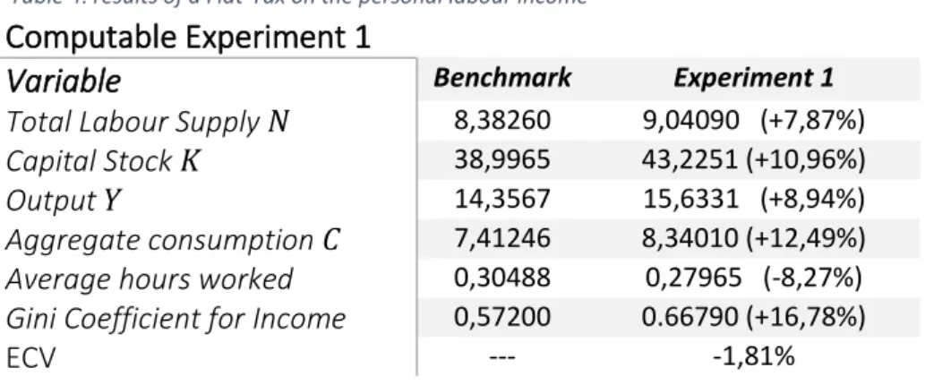
Under the reform it is observed an increase in the labour supply, as displayed in Table 4. As a consequence the aggregate output within the country increases as well, leading to a significantly higher level of aggregate consumption and savings. The Gini coefficient of the country is 0.6679, consistently increased in the experiment when compared to the Benchmark economy: this is an expected outcome, since by definition a progressive tax is a fiscal system meant to reduce the inequalities within a country. Despite the overall apparent improvement in macro aggregates, the equilibrium displays an unexpected decrease in the average hours worked and social welfare: an investigation on the causes of these effects is conducted in Chapter 6.
Computable Experiment 1
Variable Benchmark Experiment 1
Total Labour Supply 𝑁 8,38260 9,04090 (+7,87%)
Capital Stock 𝐾 38,9965 43,2251 (+10,96%)
Output 𝑌 14,3567 15,6331 (+8,94%)
Aggregate consumption 𝐶 7,41246 8,34010 (+12,49%)
Average hours worked 0,30488 0,27965 (-8,27%)
Gini Coefficient for Income 0,57200 0.66790 (+16,78%)
ECV --- -1,81%
5.2 Result of the second experiment: a Flat Tax on the personal labour and capital income The second Computational Experiment is conducted similarly to the first one: it consists in simulating a Flat-Tax with the same marginal rate for both the personal labour and capital income. If 𝜏𝑦
pag. 28 represents this marginal rate, the problem that faces an household earning more than the poverty level becomes so: 𝑣𝑡(𝑎, ƞ, 𝑖, 𝑗) = 𝑚𝑎𝑥 𝑐,𝑎′,𝑙 (𝑢(𝑐, 1 − 𝑙) + 𝛽𝜓𝑗∫ 𝑣𝑡+1(𝑎 ′, ƞ′, 𝑖, 𝑗 + 1)𝑄(ƞ, 𝑑ƞ′)) subject to: (1 + 𝜏𝑐,𝑡 )𝑐 + 𝑎′= (1 − 0.66𝜏𝑠𝑠,𝑡) 𝑤𝑡 1+0.33𝜏𝑠𝑠,𝑡ԑ𝑗𝛼𝑖ƞ𝑙𝑡+ (1 + 𝑟𝑡)(𝑎 + 𝑇𝑟𝑡) − 𝑇[𝑦𝑡] for 𝑗 < 𝑗𝑟, (1 + 𝜏𝑐,𝑡 )𝑐 + 𝑎′= 𝑆𝑆𝑡+ (1 + 𝑟𝑡(1 − 𝜏𝑦)) (𝑎 + 𝑇𝑟𝑡) − 𝜏𝑦𝑆𝑆𝑡 for 𝑗 ≥ 𝑗𝑟. (33) 𝑇[𝑦𝑡] = −( 𝑝 ∗ 𝒯 − 𝑦𝑡− 𝑟𝑡(𝑎𝑡+ 𝑇𝑟𝑡)) 𝑖𝑓 𝑦𝑡+ 𝑟𝑡(𝑎𝑡+ 𝑇𝑟𝑡) ≤ 𝑝 ∗ 𝒯 𝜏𝑦(𝑦𝑡+ 𝑟𝑡(𝑎𝑡+ 𝑇𝑟𝑡)) 𝑖𝑓 𝑦𝑡+ 𝑟𝑡(𝑎𝑡+ 𝑇𝑟𝑡) > 𝑝 ∗ 𝒯 (34)
The marginal rate found is 23%: the stationary equilibrium reports a parameter of 1,053, that means the maximum amount of minimum income granted in the economy is the 105,3% of the poverty threshold.
A graphical representation of the Lorenz curve is plotted in Figure 5, and the Gini coefficient is computed as the ratio of the area that lies between the perfect equality and this curve.
As in the first Computational Experiment this reform (look Table 5) apparently seems to boost the economy, despite then displaying lower average number of hours worked and social welfare: the
pag. 29 increase in the aggregate labour supply brings a to higher aggregate output within the country, and as a consequence to higher level of consumption and savings. Again, the flat fiscal system results in a higher income inequality in the economy, with a Gini coefficient of 0,6654
Computable Experiment 2
Variable Benchmark Experiment 2
Total Labour Supply 𝑁 8,38260 8,81568 (+5,52%)
Capital Stock 𝐾 38,9965 41,3002 (+5,59%)
Output 𝑌 14,3567 15,1356 (+5,43%)
Aggregate consumption 𝐶 7,41246 7,99237 (+7,82%)
Average hours worked 0,30488 0,25221 (-0,17%)
Gini Coefficient for Income 0,57200 0,66542 (+16,33%)
ECV --- -5,78%
6 Discussing the results
In order to better analyze the effects of these fiscal reforms and to understand how the new tax code impact the agents in different cohort ages, this chapter compares the post-reform distributions of asset holdings, labour supply, labour earnings and consumption for different cohort ages to the pre-reform ones. The discussion is conduct on the average distributions over life cycle.
6.1 First experiment: 20% Flat-Tax on the individual labour income
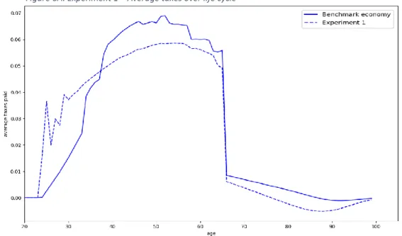
The average capital and labour eanings taxes paid by agents in different cohort ages are plotted in
Figure 6A for the benchmark economy (continuous line) and the Computational Experiment 1 (dotted Table 5: results of a Flat-Tax reforming the personal labour and capital income
pag. 30 line). The distribution is computed including the minimum income amount granted to the agents earning less than the previously calibrated threshold. It appears that agents under the age of 37 face a higher fiscal burden, while in other cohort ages they pay significantly lower taxes.
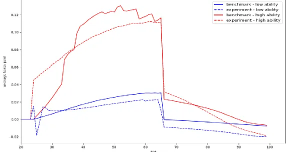
In Figure 6B the effect of the fiscal reform on taxes paid are separated above low and high skilled agents over life cycle: high level workers under 37 face significantly higher taxes, and significantly lower after that age. The average tax on the other hand decreases for low skilled workers basically for every age due to the increase in the minimum income level, by the moment they are the ones benefitting the most from it.
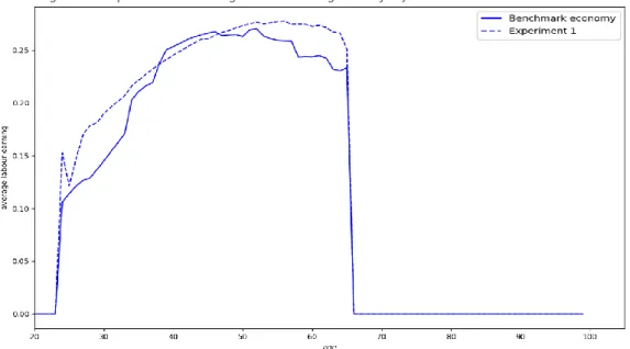
The average hours worked for different cohort ages is displayed in Figure 7A. As expected from the results previously observed and reported in Table 4, the average hors worked seems to drop consistently for basically every age level, with some exception for the early aged agents.
Figure 7A: Experiment 1 - Average hours of labour supplied over life cycle Figure 6B: Experiment 1 – Average taxes over life cycle per ability type